在信號源不足環境下手機的定位和軌跡追蹤演算法

全文

(1)國立交通大學電信工程學系碩士論文在信號源不足環境下手機的定位和軌跡追蹤演算法 Wireless Location Tracking Algorithm for Environments with Insufficient Signal Sources 研究生：林育群指導教授：方凱田. 中. 華. 民. 國九十六年六月.

(2) 在信號源不足環境下手機的定位和軌跡追蹤演算法. Wireless Location Tracking Algorithm for Environments with Insufficient Signal Sources. 研究生：林育群. Student：Yu-Chun Lin. 指導教授：方凱田. Advisor：Kai-Ten Feng. 國立交通大學電信工程學系碩士班碩士論文. A Thesis Submitted to Department of Communication Engineering College of Electrical Engineering and Computer Science National Chiao Tung University in partial Fulfillment of the Requirements for the Degree of Master in Communication Engineering June 2007 Hsinchu, Taiwan, Republic of China. 中華民國 96 年 6 月.

(3) 在信號源不足環境下手機的定位和軌跡追蹤演算法. 研究生: 林育群. 指導教授:方凱田. 國立交通大學電信工程學系. 電信研究所碩士班. 摘要手機的定位和軌跡追蹤在近年來受到相當高的注意。手機和基地台之間傳送的無線電訊號，在一般的網路定位估測機制下被廣泛地使用。此外，定位估測器加上卡曼爾濾波(Kalman filtering)的技術，可同時獲得位置的估測並且追蹤手機的軌跡。然而，這些已經存在的估測機制，在信號源不足(基地台數目小於三) 的情況下，會變得無法計算並預測手機的位置跟軌跡。在此篇論文中，有兩種可預測的定位和軌跡追蹤演算法被提出來解決這個問題。預測定位追蹤機制 ( Predictive Location Tracking (PLT) scheme) 利用從卡曼爾濾波器(Kalman Filter)的預測訊息，提供給定位估測器當作是額外的訊號輸入，彌補訊號源不足而無法計算的問題。更進一步，地理輔助的預測定位追蹤機制 (Geometric-assisted Predictive Location Tracking (GPLT) scheme)更加入了幾何精度稀釋(Geometric Dilution of Precision (GDOP))的資訊到演算法裡。採用所提出的地理輔助的預測定位追蹤(GPLT)機制在手機的定位追縱上都可獲得更好的正確率，特別是當訊號源不足的時候。在此篇論文中有許多模擬的結果來證明地理輔助的預測定位追蹤(GPLT)機制跟其他兩種網路定位追蹤機制比較，可以獲得較高的正確率和穩定性。.

(4) Wireless Location Tracking Algorithms for Environments with Insufficient Signal Sources. Advisor: Kai-Ten Feng. Student: Yu-Chun Lin. Department of Communication Engineering National Chiao Tung University. Abstract Location estimation and tracking for the mobile devices have attracted a significant amount of attention in recent years. The network-based location estimation schemes have been widely adopted based on the radio signals between the mobile device and the base stations. The location estimators associated with the Kalman filtering techniques are exploited to both acquire location estimation and trajectory tracking for the mobile devices. However, most of the existing schemes become unapplicable for location tracking due to the deficiency of signal sources. In this thesis, two predictive location tracking algorithms are proposed to alleviate this problem. The Predictive Location Tracking (PLT) scheme utilizes the predictive information obtained from the Kalman filter in order to provide the additional signal inputs for the location estimator. Furthermore, the Geometric-assisted Predictive Location Tracking (GPLT) scheme incorporates the Geometric Dilution of Precision (GDOP) information into the algorithm design. Persistent accuracy for location tracking can be achieved by adopting the proposed GPLT scheme, especially with inadequate signal sources. Numerical results demonstrate that the GPLT algorithm can achieve better precision in comparison with other network-based location tracking schemes..

(5) 誌謝. 本篇論文的完成，誠摯地感謝我的指導老師方凱田博士，從踏入交通大學電信所開始，多虧老師的循循善誘，不但給予我在課業、研究上的幫助，使我學到了分析問題及解決問題的能力。在此，僅向老師及老師的家人致上最高的感謝之意。. 感謝在電信研究所的日子裡，實驗室所提供完善的研究資源。承蒙仲賢和建華學長的提攜與照顧。而實驗室的同伴，文俊、柏軒跟裕彬，還有學弟們林志、伯泰、信龍跟瑜智，在課業上的砥礪與生活上的幫助也讓我在忙碌的研究所生涯中仍舊擁有快樂的心情。大學朋友和我的室友，志剛、柏昇、介遠、耀鈞和政達等，平日陪我打球運動，有空的時候出去玩樂，使得研究生活不只是只有苦悶，也多了許多的回憶。. 最後，感謝我的家人和我的女朋友仁雅，溫暖的家一直是我求學生涯中最強而有力的後盾，感謝你們的努力讓我能夠無後顧之憂地汲取知識，繼續升學。僅將本論文獻給我敬愛的父母，林連進先生、莊豔芬女士。. 林育群民國九十六年六月於新竹.

(6) Contents 1 Introduction. 3. 2 Preliminary studies and Related Work. 8. 2.1. Mathematical Modeling . . . . . . . . . . . . . . . . . . . . . . . . . . . . . . .. 8. 2.2. Sources of Ranging Errors . . . . . . . . . . . . . . . . . . . . . . . . . . . . . .. 9. 2.3. Studies on Existing Location Estimation Algorithms . . . . . . . . . . . . . . . 10 2.3.1. 2.4. Two-Step Least Square . . . . . . . . . . . . . . . . . . . . . . . . . . . 13. Studies on Existing Location Tracking Algorithms . . . . . . . . . . . . . . . . 17 2.4.1. Kalman Filtering . . . . . . . . . . . . . . . . . . . . . . . . . . . . . . . 17. 2.4.2. Kalman Tracking (KT) Algorithm . . . . . . . . . . . . . . . . . . . . . 18. 2.4.3. Cascade Location Tracking (CLT) Algorithm . . . . . . . . . . . . . . . 21. 3 Architectural Overview of the Proposed PLT and GPLT Algorithms. 22. 4 Formulation of the PLT Algorithm. 27. 4.1. The Two-BSs Case . . . . . . . . . . . . . . . . . . . . . . . . . . . . . . . . . . 29. 4.2. The Single-BS Case. . . . . . . . . . . . . . . . . . . . . . . . . . . . . . . . . . 30. 5 Formulation of the GPLT Algorithm. 33. 5.1. The Geometric Dilution of Precision (GDOP) . . . . . . . . . . . . . . . . . . . 33. 5.2. The Two-BSs Case . . . . . . . . . . . . . . . . . . . . . . . . . . . . . . . . . . 34 5.2.1. The Computation of the Angle θk. 5.2.2. LT . . . . . . . . . . . . . . . . . . . . 36 The Selection of the Distance rvGP 1 ,k. 1. . . . . . . . . . . . . . . . . . . . . . 35.

(7) 5.3. The Single-BS Case. . . . . . . . . . . . . . . . . . . . . . . . . . . . . . . . . . 40. 6 Performance Evaluation. 42. 6.1. The Noise Models and the Simulation Parameters . . . . . . . . . . . . . . . . . 42. 6.2. Validation of the GPLT Scheme . . . . . . . . . . . . . . . . . . . . . . . . . . . 43. 6.3. 6.2.1. Validation with Angle Effect . . . . . . . . . . . . . . . . . . . . . . . . 43. 6.2.2. Validation with Distance Effect . . . . . . . . . . . . . . . . . . . . . . . 47. Simulation Results . . . . . . . . . . . . . . . . . . . . . . . . . . . . . . . . . . 48. 7 Conclusion. 55. 2.

(8) Chapter 1. Introduction Wireless location technologies, which are designated to estimate the position of a Mobile Station (MS), have drawn a lot of attention over the past few decades. The Quality-of-Service (QoS) of the positioning accuracy has been announced after the issue of the emergency 911 (E-911) subscriber safety service [1]. With the assistance of the information derived from the positioning system, the required performance and objectives for the targeting Mobile Station (MS) can be achieved with augmented robustness. In recent years, there are increasing demands for commercial applications to adopt the location information within their system design, such as the navigation systems, the location-based billing, the health care systems, the Wireless Sensor Networks (WSNs) [2]- [4], and the Intelligent Transportation Systems (ITS) [5] [6]. With the emergent interests in the Location-Based Services (LBSs), the location estimation algorithms with enhanced precision become necessitate for the applications under different circumstances. A variety of wireless location techniques have been investigated [7]- [10]. To simplify the introduction of these techniques, in the following we use two-dimensional (2D) cases as application examples. The network-based location estimation schemes have been widely proposed and employed in the wireless communication system. These schemes locate the position of a MS based on the measured radio signals from its neighborhood Base Stations (BSs). The representative algorithms for the network-based location estimation techniques. 3.

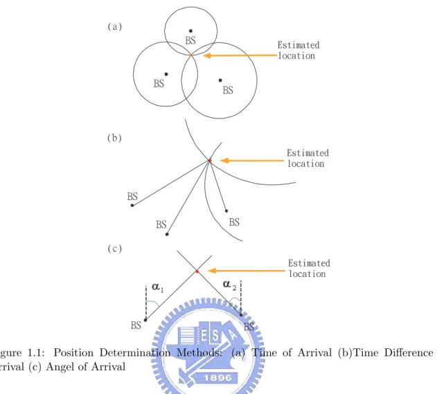
(9) )b* CT. Ftujnbufe mpdbujpo. CT. CT. )c* Ftujnbufe mpdbujpo. CT CT. CT )d*. Ftujnbufe mpdbujpo. CT. CT. Figure 1.1: Position Determination Methods: (a) Time of Arrival (b)Time Difference of Arrival (c) Angel of Arrival are the Time-Of-Arrival (TOA), the Time Difference-Of-Arrival (TDOA), and the Angle-OfArrival (AOA). The TOA scheme measures the arrival time of the radio signals coming from different wireless BSs, as shown in Fig. 1.1a; while the TDOA scheme measures the time difference between the radio signals, as shown in Fig. 1.1b. The AOA technique is conducted within the BS by observing the arriving angle of the signals coming from the MS, as shown in Fig. 1.1c. It is recognized that the equations associated with the network-based location estimation schemes are inherently nonlinear. The uncertainties induced by the measurement noises make it more difficult to acquire the estimated MS position with tolerable precision. The Taylor Series Expansion (TSE) method was utilized in [11] to acquire the location estimation of the MS from the TOA measurements. The method requires iterative processes to obtain the. 4.

(10) location estimate from a linearized system. The major drawback of the TSE scheme is that it may suffer from the convergence problem due to an incorrect initial guess of the MS’s position. The two-step LS method was adopted to solve the location estimation problem from the TOA [12], the TDOA [13], and the TDOA/AOA measurements [14]. It is an approximate realization of the Maximum Likelihood (ML) estimator and does not require iterative processes. The two-step Least Square (LS) scheme is advantageous in its computational efficiency with adequate accuracy for location estimation. Instead of utilizing the Circular Line of Position (CLOP) methods (e.g. the TSE and the two-step LS schemes), the Linear Line of Position (LLOP) approach is presented as a new interpretation for the cell geometry from the TOA measurements. Since the pairwise intersections of N TOA measurements will establish (N − 1) independent linear lines, the LS method can therefore be applied to estimate the position of the MS. The detail algorithm of the LLOP approach can be obtained by using the TOA measurements as in [15], and the hybrid TOA/AOA measurements in [16]. In addition to the estimation of a MS’s position, trajectory tracking of a moving MS has been studied [17] - [21]. The technique by combining the Kalman filter with the Weighted Least Square (WLS) method is exploited in [17]. The Kalman Tracking (KT) scheme [18] [19] distinguishes the linear part from the originally nonlinear equations for location estimation. The linear aspect is exploited within the Kalman filtering formulation; while the nonlinear term is served as an external measurement input to the Kalman filter. The technique utilized in [20] adopted the Kalman filters for both pre-processing and post-processing in order to both mitigate the Non-Line-of-Sight (NLOS) noises and track the MS’s trajectory. The Cascade Location Tracking (CLT) scheme as proposed in [21] utilizes the two-step LS method for initial location estimation of the MS. The Kalman filtering technique is employed to smooth out and to trace the position of the MS based on its previously estimated data. The Geometric Dilution of Precision (GDOP) [22] [23] and the Cram´er-Rao Lower Bound (CRLB) [24] are the well-adopted metrics for justifying the accuracy of location estimation based on the geometric layouts between the MS and its associated BSs. It has been indicated in [25] that the environments with ill-conditioned layouts will result in relatively larger. 5.

(11) GDOP and CRLB values. In general, the ill-conditioned situations can be classified into two categories: (i) insufficient number of available neighborhood BSs around the MS; and (ii) the occurrence of collinearity or coplanarity between the BSs and the MS. It is noticed that the problem caused by case (ii) can be resolved with well-planned locations of the BSs. Nevertheless, the scenarios with insufficient signal sources (i.e. case (i)) can happen in real circumstances, e.g. under rural environments or city valley with blocking buildings. It will be beneficial to provide consistent accuracy for location tracking under various environments. However, the wireless location tracking problem with deficient signal sources has not been extensively addressed in previous studies. In the cellular-based networks, three BSs are required in order to provide three signal sources for the TOA-based location estimation. The scheme as proposed in [26] considers the location tracking problem under the circumstances with short periods of signal deficiency, i.e. occasionally with only two signal sources available. The linear predictive information obtained from the Kalman filter is injected into its original LS scheme while one of the BSs is not observable. However, this algorithm is regarded as a preliminary design for signal deficient scenarios, which does not consider the cases while only one BS is available for location estimation. Insufficient accuracy for location estimation and tracking of the MS is therefore perceived. In this thesis, a Predictive Location Tracking (PLT) algorithm is proposed to improve the problem with insufficient measurement inputs, i.e. with only two BSs or a single BS available to be exploited. The predictive information obtained from the Kalman filter is adopted as the virtual signal sources, which are incorporated into the two-step LS method for location estimation and tracking. Moreover, a Geometric-assisted Predictive Location Tracking (GPLT) scheme is proposed by adopting the Geometric Dilution of Precision (GDOP) [22] concept into its formulation in order to further enhance the performance of the original PLT algorithm. The position of the virtual signal sources are relocated for the purpose of achieving the minimum GDOP value associated with the MS’s position. Along with the acquisition of the optimal location for the virtual signal source, the corresponding estimation and tracking errors acquired by using the proposed GPLT scheme can therefore be reduced. Moreover,. 6.

(12) consistent precision for location tracking of a MS is also observed by exploiting the GPLT algorithm. Comparing with the existing techniques, the simulation results show that the proposed GPLT scheme can acquire higher accuracy for location estimation and tracking even under the situations with inadequate signal sources. The remainder of this thesis is organized as follows. The related work, including the mathematic modeling, the sources of ranging errors, and other existing location estimation algorithms, is briefly described in chapter 2. The overview and motivations of the proposed Predictive Location Tracking (PLT) and Geometric-assisted Predictive Location Tracking (GPLT) schemes are explained in chapter 3. Chapter 4 presents the PLT algorithm with two different scenarios; while the formulation of the GPLT scheme is exploited in chapter 5. Chapter 6 illustrates the performance evaluation of the proposed GPLT and the PLT schemes in comparison with the existing location tracking techniques. Chapter 7 draws the conclusions.. 7.

(13) Chapter 2. Preliminary studies and Related Work 2.1. Mathematical Modeling. In order to facilitate the design of the proposed PLT and the GPLT algorithms, the signal model for the TOA measurements is utilized. The set rk contains all the available measured relative distance at the k th time step, i.e. rk = {r1,k , . . . , ri,k , . . . , rNk ,k }, where Nk denotes the number of available BSs at the time step k. The measured relative distance (ri,k ) between the MS and the ith BS (obtained at the k th time step) can be represented as. ri,k = c · ti,k = ζi,k + ni,k + ei,k. i = 1, 2, ..., Nk. (2.1). where ti,k denotes the TOA measurement obtained from the ith BS at the k th time step, and c is the speed of light. ri,k is contaminated with the TOA measurement noise ni,k and the Non-line-of-sight (NLOS) error ei,k . It is noted that the measurement noise ni,k is in general considered as zero mean with Gaussian distribution. On the other hand, the NLOS error ei,k is modeled as exponentially-distributed for representing the positive bias due to the non-lineof-sight effect [27] [28]. The noiseless relative distance ζi,k (in (2.1)) between the MS’s true. 8.

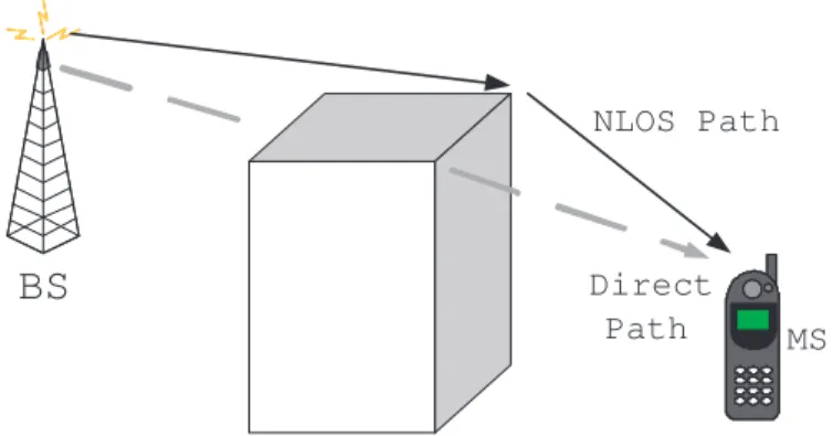
(14) NLOS Path. BS. Direct Path. MS. Figure 2.1: Geometry of the NLOS Error position and the ith BS can be obtained as 1. ζi,k = [(xk − xi,k )2 + (yk − yi,k )2 ] 2. (2.2). where xk = [xk yk ] represents the MS’s true position and xi,k = [xi,k yi,k ] is the location of the ith BS for i = 1 to Nk . Therefore, the set of all the available BSs at the k th time step can be obtained as PBS,k = {x1,k , . . . , xi,k , . . . , xNk ,k }.. 2.2. Sources of Ranging Errors. The location accuracy can be reduced due to the influence of the measurement noises. Several main sources of ranging errors are described in this section, which are referred to [29]. Non-Line-of-Sight Errors In dense urban environment, there may be no direct path from the MS to the BS as shown in Fig. 2.1. Due to reflection and diffraction, the propagating wave may actually travel excess path lengths on the order of hundreds of meters and the direct path is blocked. This phenomenon, which we refer to as the NLOS error, ultimately translates into a biased estimate of the mobile’s location. This problem has been recognized as a killer issue for mobile location. In order to mitigate the effect of the measurement bias, it is necessary to develop location algorithms that are robust to the NLOS error.. 9.

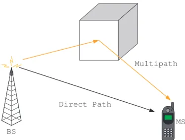
(15) Multipath. Direct Path MS BS. Figure 2.2: Multiple Reflections Arrive at the MS with Different Time Delays Multipath Errors Multipath effects are caused by reflected signals entering the receiver antenna along with direct path signal, as shown in Fig. 2.2. Since the reflected path is longer than the direct path, the multipath signal blurs the peak of the direct signal at the output of the receiver correlation channel and distorts the pseudorange measurement. Receiver Measurement Processing Advances in digital processing technology have enabled the implementation of small, affordable multiple channel receivers for parallel tracking of more than the minimum reference points for navigation solutions. This technology, in conjunction with advances in the speed and precision of microprocessor computations, has resulted in great reductions in receiver range measurement processing errors.. 2.3. Studies on Existing Location Estimation Algorithms. Different location estimation schemes have been proposed to acquire the MS’s position. Various types of information (e.g. the signal traveling distance, the received angle of the signal, or the Receiving Signal Strength (RSS)) are involved to facilitated the algorithm design for 10.

(16) location estimation. The primarily objectives in most of the location estimation algorithms are to obtain higher estimation accuracy with promoted computational efficiency. The superresolution (or high-resoluction) schemes are proposed as in [30] - [33]. The scheme studied in [30] considers arbitrary-located antennas and a particular covariance matrix within a noisy environment. The covariance matrix is composed of various types of properties, including gain, phase, frequency, polarization, and AOA information. The subspace method is proposed in the scheme generates these component estimates of the covariance metrix based on an eigen-analysis or eigen-composition. The most well-known super-resolution algorithm is the MUltiple SIgnal Classification (MUSIC) [31], It is experimentally illustrated to be a robust solution for location estimation, especially for a near-far environment. However, it has also be shown in [32] and [33] that the drawbacks of the MUSIC approach include (i) comparably high sensitivity to large noise and (ii) its complexity in computation. The beamforming system is a space-time processor that operates on the output of a sensor array. It provides spatial filtering capability by enhancing the amplitude of a coherent signal associated with surrounding noises. Since the conventional beamforming technique is sensitive to the estimation error for the MS’s position, a combination of localization and beamforming is proposed as in [34]. It increases the robustness to location errors without sacrificing the computation efficiency. An enhanced algorithm for simultaneous multi-source beamforming and adaptive multi-target tracking is studied in [35]. The correlation between the adaptive minimum variance beamforming and the optimal source localization is also investigated and developed as in [36]. Instead of exploiting the spatial and temporal information of the signal, the location fingerprinting technique locates the MS based on the the RSS [37] [38]. The technique involves both the off-line and the on-line phases. A location grid that is related to a signal signature database for a specific service area is developed in the off-line phase; while a measured RSS vector at the MS is delivered to the central server to compare with the location grid in the online phase. In addition, a hybrid algorithm which combines the RF propagation loss model is proposed to both mitigate the requirement of the training data and to adjust the configuration. 11.

(17) changes [39]. On the other hand, the ray-tracing and ray-launching techniques are the two ray optical approaches for location estimation. The radio signals that are launched from a transmitter and reflected or diffracted by various objects are aggregated in a receiver. The field strength and the signal propagation can therefore be predicted [40]; while [41] proposed an efficient algorithm for prediction. The three dimensional indoor radio propagation models are developed in [42] and [43]. Experimental formulas from extensive measurements of urban and suburban propagation losses are studied as in [44] [45]. There are also different approaches adopting linearized methods to acquire the computing efficiency while obtaining an approximate estimation of the MS’s position. The Taylor Series Expansion (TSE) method was utilized in [46] to acquire the location estimation from the TDOA measurements. The method requires iterative processes to obtain the location estimate from a linearized system. The major drawback of this method is that it may suffer from the convergence problem due to an incorrect initial guess of the MS’s position. The two-step LS method was adopted to solve the location estimation problem from the TOA [12], the TDOA [13], and the TDOA/AOA measurements [14]. It is an approximate realization of the Maximum Likelihood (ML) estimator and does not require iterative processes. The twostep LS scheme is advantageous in its computational efficiency with adequate accuracy for location estimation. However, the scheme is demonstrated to be feasible for acquiring the MS’s position under the LOS situations. Instead utilizing the Circular Line Of Position (CLOP) methods (e.g. the TSE and twostep LS schemes), the Linear Line Of Position (LLOP) approach is presented as a new interpretation for the cell geometry from the TOA measurements. Since two TOA measurements that intersect at two points will generate a connecting line, two independent lines will be created by using three BSs in the scenario of two-dimensional location estimation. Therefore, the LS method can be adopted to estimate the location of the MS. The detail algorithm of the LLOP approach can be obtained by using the TOA measurements as in [15], and the hybrid TOA/AOA measurements in [16]. Some well-known schemes are improved continuously in order to achieve higher accu-. 12.

(18) racy or promote the computational efficiency. The famous linear time-based algorithms, the Taylor-Series Estimation (TSE) [46], the two-step LS method, and the Linear Line-of-Position (LLOP) [15], are briefly described in the following subsection. For simplification, the thesis only described the two-step LS method in two-dimensional plane.. 2.3.1. Two-Step Least Square. The content of this section will show the Two-step Least Square (two-step LS) location algorithm for TOA measurements and it can be obtained in [12]. For simplification, the two-step LS method will be described for TOA measurements in a two-dimensional (2-D) plane. The two-step LS method for TDOA measurements can be derived from the similar concept. Assuming that (xk , yk ) is the position of the mobile device, (xi,k , yi,k ) is the position of the ith BS and ri,k is the TOA measurement from the BSi . Since in practice, especially in urban or in mountainous areas, the signals from the mobile device are usually unable to arrive at the base stations directly (or in the oppositive direction), they always take a longer path than the direct one. So by incorporating the influences of NLOS propagation, killer issue for location estimation, on the location estimation, there exists 2 2 ri,k ≥ (xi,k − xk )2 + (yi,k − yk )2 = κi,k − 2xi,k xk − yi,k yk + x2i,k + yi,k. i = 1, 2, ...N (2.3). 2 . r where κi,k = x2i,k + yi,k i,k = cti,k is the measured distance between the MS and the ith BS, (1). and c is the speed of light. By defining a new variable βk. (1)2. = xk. (1)2. + yk. , we rewrite (2.3). through a set of linear expressions 2 −2xi,k xk − 2yi,k yk + βk ≤ ri,k − κi,k. (1). (1). Let z k = [ˆ xk. (1). yˆk. i = 1, 2, ...N. (2.4). (1) βˆk ]T and express (2.4) in matrix form. (1). Hk z k ≤ Jk. 13. (2.5).

(19) where.   −2x1,k   −2x2,k  Hk =   .   −2xN,k. − 2y1,k − 2y2,k .. .. − 2yN,k.  1   1       1. .  2 r − κ 1,k   1,k    r2 − κ2,k   2,k  Jk =     .     2 rN,k − κN,k. With measurement noise, the error vector is (1). ψk = Jk − Hk z k. (2.6). When ri,k can be expressed as ξi,k + cni,k , the error vector ψk is found to be ψk = 2cBk nk + c2 nk ¯ nk Bk = diag{ξ1,k , ξ2,k , ..., ξN,k }. (2.7). The symbol ¯ represents the Schur product (element-by-element product). In addition, the second term on the right of (2.7) can be ignored since the condition cni,k ≤ ξi,k is usually satisfied. As a result, ψk becomes a Gaussian random vector with covariance matrix given by Ψk = E[ψk ψkT ] = 4c2 Bk Qk Bk. (2.8). Qk is the covariance matrix of measured noise, and ξ1,k ,...,ξN,k are denoted as the true values of (1). distances between the sources and the receiver. The element x k are related by the equation, (1). (1)2. βk = xk. (1)2. + yk. , which means that (2.5) is still a set of nonlinear equations in two variables. xk and yk . The approach to solve the nonlinear problem is to first assume that there is (1). (1). no relationship among xk , yk. (1). and βk . That can then be solved by Least Square (LS).. The final solution is obtained by imposing the known relationship to the computed result via another LS computation. This two step procedure is an approximation of a true ML. 14.

(20) (1). (1). estimator. By considering the elements of x k independent, the ML estimator of x k is (1). xk. = arg min{(Jk − Hk x k )T Ψ−1 k (Jk − Hk x k )} −1 T −1 = (HTk Ψ−1 k Hk ) Hk Ψk Jk. (1). (2.9) (1). (1). (1). The covariance matrix of x k is obtained by evaluating the expectations of x k and (x k )(x k )T (1). from (2.9). The covariance matrix of x k can be calculated as [13] (1). −1 cov(x k ) = (HTk Ψ−1 k Hk ). (2.10). (1) (1) (1) Since we have used the independent supposition of variables xˆk , yˆk , and βˆk in the (1). estimation of x k. (1) (1) (1) though the variable βˆk is dependent on the variable x ˆk and yˆk , we. (1) (1) (1) should revise the results as follows. Let the estimation errors of xˆk , yˆk , and βˆk be e1,k ,. e2,k , and e3, . Here and below, denote the `th entry of a matrix M as [M ]` ; then the entries in (1). vector x k become (1). (2.11a). (1). (2.11b). (1). (2.11c). [x k ]1 = xo + e1,k [x k ]2 = yo + e2,k [x k ]3 = βo + e3,k. (1) (1) (1) where xo , yo , and βo are denoted as the true values of x ˆk , yˆk , and βˆk . Let another error. vector (2). ψk0 = J0k − H0k x k where. .  1.   H0k =  0  1.   (1) [x k ]21    2 J0k = [x (1)  ]  k 2 (1) [x k ]3. 0.   1   1. 15. (2.12).

(21)   (2)2 ˆk  (2) x and x k = . Substituting 2.11a- 2.11c into 2.12, we have (2)2 yˆk [ψk ]1 = 2xo e1,k + e21,k ≈ 2xo e1,k [ψk ]2 = 2yo e2,k + e22,k ≈ 2yo e2,k [ψk ]3 = e3,k Obviously, the above approximations are valid only when the errors e1,k , e2,k , and e3,k are fairly small. Subsequently, the covariance matrix of ψ 0 is (1). T. Ψ0k = E[ψk0 ψk0 ] = 4B0k cov(x k )B0k B0k = diag{xo , yo , 0.5}. (2.14). As an approximation, elements xo and yo in matrix B0k can be replaced by the first two (1). (1). elements x ˆk and yˆk. (1). (2). in x k . Similarly, the ML estimate of x k is given by (2). xk. T. −1. −1. T. −1. T. −1. (1). −1. T. −1. (1). −1. = (H0k Ψ0k Hk0 )H0k Ψ0k J0k. (2.15) −1. ≈ (H0k B0k (cov(x k ))−1 B0k H0k ) •. (H0k B0k (cov(x k ))−1 B0k )J0k. So the final position estimation z k = [ˆ xk zk =. q (2) xk ,. (2.16) (2.17). yˆk ]T is q (2) zk = − xk. or. (2.18). (1). Here the sign of x ˆk should coincide with the sign of [x k ]1 calculated by solving (2.9), and (1). the sign of yˆk coincides with the sign of [x k ]2 . The complete derivation of the two-step LS for TOA measurements is shown above. In addition, the two-step LS method can be adopted to estimate MS location from the TDOA [13], and the TDOA/AOA measurements [14]. The following two subsections describe the 3-D 16.

(22) TOA location estimation for the satellite-based system, and the 3-D TDOA/AOA location estimation algorithm for the cellular network.. 2.4 2.4.1. Studies on Existing Location Tracking Algorithms Kalman Filtering. Kalman Filtering method is always utilized for location tracking because it utilizes the state vector with the position, the velocity, and the acceleration of the MS to record and predict the MS’s trajectory. The measurement and state equations for the Kalman filter can be represented as. z k = Mˆ sk + mk. (2.19). sˆ k = Fˆ s k−1 + p k. (2.20). The matrix M in the measurement equation (2.19) relates the state to the measurement z k . The matrix F in the equation (2.20) relates the state at the previous time step k-1 to the state at the current step k. The variables m k and p k denote the measurement and the process noises associated with the covariance matrices R and Q within the Kalman filtering formulation. The Kalman filter estimates a process by using a form of feedback control: the filter estimates the process state at some time and then obtains feedback in the form of (noisy) measurements. As such, the equations of the Kalman filter fall into two groups: time update equations and measurement update equations. The time update equations are as following. sˆ k|k−1 = Fˆ s k−1|k−1. (2.21). Pk|k−1 = FPk−1|k−1 F + Q. (2.22). 17.

(23) And the measurement update equations are shown Kk = Pk|k−1 MT (MPk|k−1 MT + R)−1. (2.23). sˆ k|k = sˆ k|k−1 + Kk (z k − Mˆ s k|k−1 ). (2.24). Pk|k = (I − Kk M)Pk|k−1. (2.25). The first task during the measurement update os to compute the Kalman gain, Kk . The next step is to actually measure the process to obtain z k , and then to generate a posteriori state estimate by incorporating the measurement as in (2.24). The final step is to obtain a posteriori error covariance estimate via (2.25). The Kalman filter instead recursively conditions the current estimate on all of the past measurements.. 2.4.2. Kalman Tracking (KT) Algorithm. The Kalman Tracker [18], which is designed based on the TDOA measurements, considers the nonlinear term as an external measurement input to its Kalman filtering formulation. The Kalman Tracking method for TOA measurements can be derived from the similar concept. It distinguishes the linear part from the originally nonlinear equations for location estimation and tracking. The difference between ranges of the ith BS and the reference BS can be defined as. ri,1,k = ri,k − r1,k = c · ti,1,k. i = 2, ..., N. (2.26). where c is the propagation speed, and N is the number of active BSs. The squared distance between the ith BS and the MS is equal to 2 ri,k = ||xi,k − xk ||2 = ||x2i,k || − 2xTi,k xk + ||xk ||2. where xi,k = [ˆ xi,k. yˆi,k ]T and xk = [xk. (2.27). yk ]T are the vectors which define the known position. of the ith BS and unknown MS position.. 18.

(24) These equations show a nonlinear relation between the TDOA measurements and the BS position. From (2.26), the squared distance between the ith BS and the BS can also be expressed as 2 2 2 ri,k = ri,1,k + 2r1,k ri,1,k + r1,k. (2.28). Using equations (2.27) and (2.28), the linear system of equations is derived as. Gk xk = uk − r1,k ρk where. (2.29). . .  (x2,k − x1,k ) (y2,k − y1,k )  Gk =  ... ...   (xN,k − x1,k ) (yN,k − y1,k ) .      . ||2. ||2. 2 r2,1,k.  ||x2,k − ||x1,k − 1 uk =  ... 2  2 ||xN,k ||2 − ||x1,k ||2 − rN,1,k . .  r2,1,k  ρk =   ...  rN,1,k.     .     . The resulting linear equation also depends on a distance measurement r1,k , proportional to the TOA between the reference BS and the MS, which has a nonlinear dependence on the BS co-ordinates. In [18], a Kalman tracker based on TDOA measurements is derived from the linear equation (2.29). The use of the Kalman filter allows tracking the position and speed of the MS. The transition equation, defined for continuous movement, is linear. ˆsk = Fˆsk−1 + pk. 19. (2.30).

(25) where ˆsk = [ˆ xk. yˆk. vˆx,k. vˆy,k ]T is the dynamic state vector, where its components represent. the MS position and the speed in two-dimensional Cartesian co-ordinates at discrete time k. The matrix F is the state matrix with 4 equal to the time interval between samples . . 1 0 4 0      0 1 0 4    F=     0 0 1 0    0 0 0 1 and p(k) = [0. 0 px,k. (2.31). py,k ] is the disturbance transition vector defined as a two-dimensional. random speed vector with covariance matrix Q. From the linear equation (2.29), it can be defined the measurement equation that relates the state vector with the observation vector. zk = Gk ˆsk + mk. (2.32). where matrix Gk is constant instead of the variable matrix derived for the Extended Kalman filter in [19] and the update equations are the same as that in the front subsection. The noise vector mk depends on the noise in the TDOA measurement o ri,1,k = ri,1,k + cni,1,k. i = 2, ..., N. (2.33). o being ri,1,k = ctoi,1,k obtained from the noise free value of the TDOA between the ith BS and. the reference BS. Substituting this expression in equation (2.29) and considering that in practice cni,1,k << o is usually satisfied, the measurement noise is found to be ri,k. mk = cBk nk. (2.34). o , r o , ..., r o } Bk = diag{r2,k N,k 3,k. (2.35). 20.

(26) with covariance matrix Ck = c2 Bk Rk Bk. (2.36). Rk is the covariance matrix of the noise in the TDOA measurments defined from the variance of the noise in the time delay estimation from each BS Rk = Hk σT2 DOA HTk. (2.37). Hk is the (N-1 )x(N ) matrix that defines the difference of times in the TDOA method . . −1 1 0 ... 0      −1 0 1 ... 0    Hk =      ... ... ... ... ...    −1 0 0 ... 1. (2.38). assuming that the measurements obtained are uncorrelated σT2 DOA is a diagonal matrix of dimension equal to the number of avalaible measurements N.. 2.4.3. Cascade Location Tracking (CLT) Algorithm. The Cascade Location Tracking (CLT) scheme as proposed in [21] utilizes the two-step Least Square (LS) method [12] [13] for initial location estimation of the MS. The two-step LS method computes the solution zk which is also the measurement input of Kalman filter. After the Kalman filter, we can get the final solution ˆsk of MS. The Kalman filtering technique is employed to smooth out and to trace the position of the MS based on its previously estimated data. The details of the two-step LS method and Kalman filter are illustrated in front sections.. 21.

(27) Chapter 3. Architectural Overview of the Proposed PLT and GPLT Algorithms The objective of the proposed Predictive Location Tracking (PLT) and the Geometric-assisted Predictive Location Tracking (GPLT) algorithms is to utilize the predictive information acquired from the Kalman filter to serve as the assisted measurement inputs while the environments are deficient with signal sources. Fig. 3.1, Fig. 3.2 and Fig. 3.3 illustrate the system architectures of the KT [18], the CLT [21] and the proposed PLT/GPLT schemes. The TOA signals (r k as in (2.1)) associated with the corresponding location set of the BSs (PBS,k ) are obtained as the signal inputs to each of the system, which result in the estimated state vector ˆ k ]T where x ˆk = [ˆ ˆk ˆk a xk yˆk ] represents the MS’s estimated position, v of the MS, i.e. sˆ k = [ˆ xk v ˆ k = [ˆ = [ˆ vx,k vˆy,k ] is the estimated velocity, and a ax,k a ˆy,k ] denotes the estimated acceleration. Since the equations (i.e.(2.1) and (2.2)) associated with the network-based location estimation are intrinsically nonlinear, different mechanisms are considered within the existing algorithms for location tracking. The KT scheme [18] (as shown in Fig. 3.1) explores the linear aspect of location estimation within the Kalman filtering formulation; while the nonlinear term (i.e. βˆk = x ˆ2k + yˆk2 ) is treated as an additional measurement input to the Kalman 22.

(28) TOA Signals PBS,k - rk. Location Estimator (2-Step LS). Nk < 3. Kalman Tracking. k. sk = [ xk vk ak ]T Figure 3.1: The Architecture Diagrams of the Kalman Tracking (KT) Scheme. TOA Signals PBS,k - rk. Location Estimator (2-Step LS) Nk < 3. zk. Kalman Filter. sk = [ xk vk ak ]T Figure 3.2: The Architecture Diagrams of the Cascade Location Tracking (CLT) Scheme. 23.

(29) TOA Signals PBS,k - rk. No. PBS,k rk. 0 < Nk < 3 ? Yes. r ke = { rk , rv, k } e PBS,k = { PBS, k , PBSv, k }. Location Estimator (2-Step LS) Nk = 0. PBSv, k - rv, k. GPLT/PLT Criterions. zk Kalman Filter. sk = [ xk vk ak ]T. Figure 3.3: The Architecture Diagrams of the Proposed Predictive Location Tracking (PLT) and Geometric-assisted Predictive Location Tracking (GPLT) Scheme filter. It is stated within the KT scheme that the value of the nonlinear term can be obtained from an external location estimator, e.g. via the two-step LS method. Consequently, the estimation accuracy of the KT algorithm greatly depends on the precision of the additional location estimator. On the other hand, the CLT scheme [21] (as illustrated in Fig. 3.2) adopts the two-step LS method to acquire the preliminary location estimate of the MS. The Kalman Filter is utilized to smooth out the estimation error by tracing the estimated state vector sˆ k of the MS. The architecture of the proposed PLT and GPLT schemes is illustrated in Fig. 3.3. It is noticed that the GPLT algorithm involves additional transformation via the GDOP calculation comparing with the PLT scheme. It can be seen that the PLT/GPLT algorithms will be the same as the CLT scheme while Nk ≥ 3, i.e. the number of available BSs is greater than or equal to three. On the other hand, the effectiveness of the PLT/GPLT schemes is revealed as 1 ≤ Nk < 3, i.e. with deficient measurement inputs. The predictive state information obtained from the Kalman filter is utilized for acquiring the assisted information, which will be fed back into the location estimator. The extended sets for the locations of the BSs (i.e. P eBS,k = {PBS,k , PBSv ,k }) and the measured relative distances (i.e. r ek = {rk , rv,k }) will be 24.

(30) utilized as the inputs to the location estimator. The sets of the virtual BS’s locations PBSv ,k and the virtual measurements rv,k are defined as follows. Definition 1 (Virtual Base Stations) Within the PLT/GPLT formulation, the virtual Base Stations are considered as the designed locations for assisting the location tracking of the MS under the environments with deficient signal sources. The set of virtual BSs PBSv ,k is defined under two different numbers of Nk as. PBSv ,k =.    {xv ,k } 1. for Nk = 2.   {xv1 ,k , xv2 ,k } for Nk = 1. (3.1). Definition 2 (Virtual Measurements) Within the PLT/GPLT formulation, the virtual measurements are utilized to provide assisted measurement inputs while the signal sources are insufficient. Associating with the designed set of virtual BSs PBSv ,k , the corresponding set of virtual measurements rv,k is defined as. rv,k =.    {rv ,k } 1. for Nk = 2.   {rv1 ,k , rv2 ,k } for Nk = 1. (3.2). It is noticed that the major tasks of both the PLT and GPLT schemes are to design and to acquire the values of PBSv ,k and rv,k for the two cases (i.e. Nk = 1 and 2) with inadequate signal sources. In both the KT and the CLT schemes, the estimated state vector sˆ k can only be updated by the internal prediction mechanism of the Kalman filter while there are insufficient numbers of BSs (i.e. Nk < 3 as shown in Fig. 3.1 and 3.2 with the dashed lines). The location estimator (i.e. the two-step LS method) is consequently disabled owing to the inadequate number of the signal sources. The tracking capabilities of both schemes significantly depend on the correctness of the Kalman filter’s prediction mechanism. Therefore, the performance for location tracking can be severely degraded due to the changing behavior of the MS, i.e. with the variations from the MS’s acceleration. On the other hand, the proposed PLT/GPLT algorithms can still provide satisfactory tracking performance with deficient measurement inputs, i.e. with Nk = 1 and 2. Under 25.

(31) these circumstances, the location estimator is still effective with the additional virtual BSs PBSv ,k and the virtual measurements rv,k , which are imposed from the predictive output of the Kalman filter (as shown in Fig. 3.3). It is also noted that the PLT/GPLT schemes will perform the same as the CLT method under the case with no signal input, i.e. under Nk = 0. Furthermore, the GPLT algorithm enhances the precision and the robustness of the location estimation from the PLT scheme by considering the GDOP effect, i.e. the geographic relationship between the locations of the BSs and the MS. By adopting the GPLT scheme, the LT locations of the virtual BSs PPBSLTv ,k obtained from the PLT method are adjusted into PGP BSv ,k. in order to make the predicted MS possess with a minimal GDOP value. Consequently, smaller estimation errors can be acquired by exploiting the GPLT algorithm comparing with the PLT scheme. The virtual BS’s location set PPBSLTv ,k and the virtual measurements rPv,kLT by exploiting the PLT formulation is presented in the next section; while the adjusted location LT set of the virtual BSs PGP BSv ,k adopting from the GPLT algorithm will be derived in chapter. 5.. 26.

(32) Chapter 4. Formulation of the PLT Algorithm The proposed Predictive Location Tracking (PLT) scheme will be explained in this section. As shown in Fig. 3.3, the measurement and state equations for the Kalman filter can be represented as. z k = Mˆ sk + mk. (4.1). sˆ k = Fˆ s k−1 + p k. (4.2). ˆ k ]T . The variables m k and p k denote the measurement and the process ˆk a where sˆ k = [ˆ xk v noises associated with the covariance matrices R and Q within the Kalman filtering formulation. The measurement vector z k = [ˆ xls,k yˆls,k ]T represents the measurement input which is obtained from the output of the two-step LS estimator at the k th time step (as in Fig. ??.(c)).. 27.

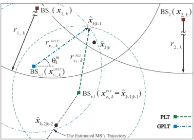
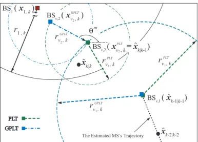
(33) BS ( x1, k ). BS2 ( x2, k ). 1. xk|k-1. . r1 , k rv , k. GPLT. r2 , k. xk|k. 1. rv , k PLT. m. θk. 1. BSv,1 ( xvGPLT ) ,k 2. BSv,1 ( xvPLT, k = xk-1|k-1) 2. PLT. xk-2|k-2. GPLT The Estimated MS’s Trajectory. Figure 4.1: The Schematic Diagram of the Two-BSs Case for the proposed PLT and GPLT Schemes The matrix M and the state transition matrix F can be obtained as   1 M =  0   1   0     0 F =    0    0   0.  0 0 0 0 0   1 0 0 0 0. (4.3) . 0 ∆t. 0. 1 2 2 ∆t. 1. 0. ∆t. 0. 0. 1. 0. ∆t. 0. 0. 1. 0. 0. 0. 0. 1. 0. 0. 0. 0. 0.       0    ∆t    0    1. 1 2 2 ∆t. (4.4). where ∆t denotes the sample time interval. The main concept of the PLT scheme is to provide additional virtual measurements (i.e. rv,k as in (3.2)) to the two-step LS estimator while the signal sources are insufficient. Two cases (i.e. the two-BSs case and the single-BS case) are considered as follows:. 28.

(34) 4.1. The Two-BSs Case. As shown in Fig. 4.1, it is assumed that only two BSs (i.e. BS1 and BS2 ) associated with two TOA measurements are available at the time step k in consideration. The main target is to introduce an additional virtual BS along with its virtual measurement (i.e. PPBSLTv ,k = P LT P LT {xPv1LT ,k } and rv,k = {rv1 ,k }) by acquiring the predictive output information from the Kalman. filter. Knowing that there are predicting and correcting phases within the Kalman filtering formulation, the predictive state can therefore be utilized to compute the supplementary virtual measurement rvP1LT ,k as rvP1LT ,k. = kˆ x k|k−1 − xˆ k−1|k−1 k = kM F sˆ k−1|k−1 − xˆ k−1|k−1 k. (4.5). where xˆ k|k−1 denotes the predicted MS’s position at time step k; while xˆ k−1|k−1 is the corrected MS’s position obtained at the (k − 1)th time step. It is noticed that both values are available at the (k − 1)th time step. The virtual measurement rvP1LT ,k is defined as the distance between the previous location estimate (ˆ x k−1|k−1 ) as the position of the virtual BS (i.e. BSv,1 : ˆ k−1|k−1 ) and the predicted MS’s position (ˆ xPv1LT x k|k−1 ) as the possible position of the MS ,k , x (as shown in Fig. 4.1). It is also noted that the corrected state vector sˆ k−1|k−1 is available at the current time step k; while sˆ k|k is unobtainable at the k th time step. By adopting rvP1LT ,k (in (4.5)) as the additional signal input, the measurement vector z k can be acquired after e the three measurement inputs rek = {r1,k , r2,k , rvP1LT ,k } and the locations of the BSs PBS,k =. {x 1,k , x 2,k , x Pv1LT ,k } have been imposed into the two-step LS estimator. Therefore, the state vector sˆ k|k can be obtained with the implementation of the correcting phase of the Kalman filter at the time step k as sˆ k|k = sˆ k|k−1 + Pk|k−1 MT [MPk|k−1 MT + R]−1 (z k − Mˆ s k|k−1 ). 29. (4.6).

(35) BS1 (. x1, k ). . r1 , k. GPLT. BSv,2 ( xv. 3 2. ,k. ) m. GPLT. rv , k. θk. 2. BSv,2 (. PLT. xv , k = xk|k-1) 3 3. PLT. rv , k. xk|k. 2. PLT. rv , k 1. BSv,1 (. GPLT. rv , k. xk-1|k-1). 1. PLT GPLT The Estimated MS’s Trajectory. xk-2|k-2. Figure 4.2: The Schematic Diagram of the Single-BS Case for the proposed PLT and GPLT Schemes where Pk|k−1 = FPk−1|k−1 FT + Q. (4.7). Pk−1|k−1 = [ I − Pk−1|k−2 MT (MPk−1|k−2 MT + R)−1 M ] Pk−1|k−2. (4.8). It is noted that Pk|k−1 and Pk−1|k−1 represent the predicted and the corrected estimation covariances within the Kalman filter. I in (4.8) is denoted as an identity matrix. As can been observed from Fig. 4.1, the virtual measurement rvP1LT ,k associating with the other two existing measurements r1,k and r2,k provide a confined region for the estimation of the MS’s location at the time step k, i.e. xˆ k|k .. 4.2. The Single-BS Case. In this case, only one BS (i.e. BS1 ) with one TOA measurement input is available at the k th time step (as shown in Fig.4.2). Two additional virtual BSs and measurements are required P LT P LT for the computation of the two-step LS estimator, i.e. PPBSLTv ,k = {xPv1LT ,k , xv2 ,k } and rv,k =. 30.

(36) P LT P LT {rvP1LT ,k , rv2 ,k }. Similar to the previous case, the first virtual measurement rv1 ,k is acquired as. ˆ k−1|k−1 ) in (4.5) by considering xˆ k−1|k−1 as the position of the first virtual BS (i.e. xPv1LT ,k = x with the predicted MS’s position (i.e. xˆ k|k−1 ) as the possible position of the MS. On the other hand, the second virtual BS’s position is assumed to locate at the predicted MS’s position (i.e. ˆ k|k−1 ) as illustrated in Fig. 4.2. The corresponding second virtual measurement xPv2LT ,k , x rvP2LT ,k is defined as the average prediction error obtained from the Kalman filtering formulation by accumulating the previous time steps as k−1. rvP2LT ,k. 1 X kˆ x i|i − xˆ i|i−1 k = k−1. (4.9). i=1. th time step. It is noted that rvP2LT ,k is obtained as the mean prediction error until the (k − 1). In the case while the Kalman filter is capable of providing sufficient accuracy in its prediction phase, the virtual measurement rvP2LT ,k may approach zero value. Associating with the single measurement r1,k from BS1 , the two additional virtual measurements rvP1LT ,k (centered ˆ k|k−1 ) result in a constrained region (as in Fig. 4.2) for at xˆ k−1|k−1 ) and rvP2LT ,k (centered at x location estimation of the MS under the environments with insufficient signal sources. It is also noticed that the variations of the measurement inputs are the required information for adopting the two-step LS estimator. It utilizes the signal variation as an indicator to consider the weighting factor for a specific signal source, i.e. smaller weighting coefficient should be assigned to a measurement input if it encompasses comparably larger signal variations. The weighted least square algorithm can therefore be performed within the twostep LS estimator according to the designated weighting values associated with the signal sources. Similar concept can be exploited to assign the weighting coefficients for the virtual measurements. The virtual measurements can be represented as. rvi ,k = ζvi ,k + nvi ,k. for i = 1, 2. (4.10). where ζvi ,k is denoted as the deterministic noiseless virtual measurement; while nvi ,k represents the virtual noise (i.e. the component with randomness) associated with the virtual. 31.

(37) measurement rvi ,k . Based on (4.5), the signal variation of rvP1LT ,k is considered as the variance of the predicted distance kˆ x k|k−1 − xˆ k−1|k−1 k between the previous (k − 1) time steps. Therefore, the virtual noise can be regarded as zero mean with variance σn2 v. 1 ,k. = Var(rvP1LT ,k ). = Var(kˆ x k|k−1 − xˆ k−1|k−1 k). It is noted that the mean value of rvPiLT ,k is considered by the noiseless virtual measurement ζvP1LT ,k . Similarly, since the signal variation of the second virtual measurement rvP2LT ,k is obtained as the variance of the averaged prediction errors (as in (4.9)), the associated virtual noise nv2 ,k can be considered as zero mean with variance σn2 v 2 = Var(rvP2LT ,k ). Consequently, the variances of the virtual noises (i.e. σnv. 1 ,k. and σn2 v. 2 ,k. 2 ,k. ) will be. exploited as the weighting coefficients within the formulation of the two-step LS estimator.. 32.

(38) Chapter 5. Formulation of the GPLT Algorithm The geometric relationship between the MS and its associated BSs (i.e. indicated by the corresponding GDOP value) will affect the precision for location estimation and tracking. The concept of the proposed GPLT scheme is to adjust the positions of the designed virtual BSs such that the predicted MS will be situated at a location with a smaller GDOP value. The modified virtual BS’s positions will therefore be adopted associated with the existing BSs for location estimation. Similarly, the two-BSs and the single-BS cases are considered as follows. First, we will explain the formulations of the GDOP shortly.. 5.1. The Geometric Dilution of Precision (GDOP). The GDOP [22] is defined as the ratio between the location estimation error and the associated measurement error. It is utilized as an index for observing the location precision of the MS under different geometric location within the networks (e.g. the cellular or the satellite networks). In general, a larger GDOP value corresponds to a comparably worse geometric layout (established by the MS and its associated BSs), which consequently results in augmented errors for location estimation. On the other hand, as the GDOP value becomes smaller, the effect from the geometric relationship to the location estimation accuracy will turn out to 33.

(39) be insignificant. Considering the MS’s location under the two-dimensional coordinate, the GDOP value (G) obtained at the position xk can be represented as © £ ¤ª 1 Gxk = trace (HTxk Hxk )−1 2. (5.1). where . Hxk.       =     .  xk −x1,k ζ1,k. yk −y1,k ζ1,k. .... .... xk −xi,k ζi,k. yk −yi,k ζi,k. .... .... xk −xNk ,k ζNk ,k. yk −yNk ,k ζNk ,k.            . (5.2). It is noted that the elements within the matrix Hxk can be acquired from (2.2). It has been shown in [22] that the minimum GDOP value frequently occurs around the center of the network layout, e.g. the minimum GDOP inside a K-side (K ≥ 3) regular polygon is shown to take place at the center of the layout and the value is obtained as G =. √2 . K. Moreover, the. GDOP value and the Cramer-Rao Lower Bound (CRLB) are demonstrated to be identical given a Gaussian-distributed noise model [23].. 5.2. The Two-BSs Case. In this case, the primary target for the GPLT scheme is to design the location of the virtual LT GP LT BS, i.e. BSv,1 : xGP v1 ,k . As shown in Fig. 4.1, two parameters (i.e. the distance rv1 ,k. and the angle θk ) w.r.t. the predicted MS’s position xˆ k|k−1 are introduced to represent the LT designed virtual BS’s position xGP v1 ,k . The selection of these two parameters within the GPLT. algorithm is explained in the following subsections.. 34.

(40) 5.2.1. The Computation of the Angle θk. LT such that the The main objective of the GPLT scheme is to acquire the angle θk of xGP v1 ,k. predicted MS (ˆ x k|k−1 ) will possess a minimal GDOP value within its network topology for location estimation. As illustrated in Fig. 4.1, the following equality can be obtained based on the geometric relationship: LT LT LT xˆ k|k−1 − xGP = (rvGP · cos θk , rvGP · sin θk ) v1 ,k 1 ,k 1 ,k. (5.3). LT As mentioned above, the position of the virtual BS (xGP v1 ,k ) is designed such that the predicted. MS (i.e. xˆ k|k−1 ) will be located at a minimal GDOP position based on the extended geometric LT set P eBS,k = {x1,k , x2,k , xGP v1 ,k }. By incorporating (1) into (5.1) and (5.2), the GDOP value. (i.e. Gxˆ k|k−1 ) computed at the predicted MS’s position xˆ k|k−1 = (ˆ xk|k−1 , yˆk|k−1 ) can be obtained. The associated matrix Hxˆ k|k−1 becomes  Hxˆ k|k−1.   =  . x ˆk|k−1 −x1,k r1,k x ˆk|k−1 −x2,k r2,k LT x ˆk|k−1 −xGP v ,k. yˆk|k−1 −y1,k r1,k yˆk|k−1 −y2,k r2,k yˆk|k−1 −yvGP,kLT. rvGP,kLT. rvGP,kLT. 1. 1. . .     =    . x ˆk|k−1 −x1,k r1,k x ˆk|k−1 −x2,k r2,k. yˆk|k−1 −y1,k r1,k yˆk|k−1 −y2,k r2,k. cos θk. sin θk. 1. 1.      . (5.4). It is noted that the noiseless relative distance ζi,k in (5.1) are approximately replaced by ri,k in (5.4) since ζi,k are considered unattainable. It can be observed from (5.4) that the matrix Hxˆ k|k−1 associated with the resulting Gxˆ k|k−1 value are regarded as functions of the angle θk , i.e. Hxˆ k|k−1 (θk ) and Gxˆ k|k−1 (θk ). Based on the objective of the GPLT scheme, the angle θkm which results in the minimal GDOP value can therefore be acquired as θkm. ( ) ½ ¾ ∂Gxˆ k|k−1 (θk ) = arg min Gxˆ k|k−1 (θk ) = arg =0 ∀θk ∂θk. (5.5). By substituting (5.4) and (5.1) into (5.5), the angle θkm can be computed as Ã θkm = tan−1. 1±. 35. ! √ 1 + Γ2 Γ. (5.6).

(41) where. Γ=. 2 (ˆ 2 (ˆ 2[r2,k xk|k−1 − x1,k )(ˆ yk|k−1 − y1,k ) + r1,k xk|k−1 − x2,k )(ˆ yk|k−1 − y2,k )]. (5.7) 2 (ˆ 2 (ˆ 2 (ˆ 2 (ˆ r2,k xk|k−1 − x1,k )2 − r2,k yk|k−1 − y1,k )2 + r1,k xk|k−1 − x2,k )2 − r1,k yk|k−1 − y2,k )2. It is noted that the noiseless relative distance ζi,k in (5.7) are replaced by ri,k for the computation of Γ since ζi,k are in general considered unattainable. At each time instant k, the LT can therefore be obtained such that x ˆ k|k−1 is relative angle θkm between xˆ k|k−1 and xGP v1 ,k. located at the position with a minimal GDOP value based on its current network layout.. 5.2.2. LT The Selection of the Distance rvGP 1 ,k. LT will be determined, which can be utilized In this subsection, the virtual measurement rvGP 1 ,k LT for acquiring the position of the virtual BS x GP v1 ,k . It is observed in (5.4) that the GDOP value. at the predicted MS’s position is primarily dominated by the relative angle (i.e. θk ) between LT ) is considered uninfluential the MS and the BSs; while the distance information (i.e. rvGP 1 ,k. to the GDOP value. This uncorrelated relationship between the GDOP value and the relative distance has also been observed as in [22]. The following Lemma shows that the selection of LT becomes insignificant for the WLS-based location estimation. the distance rvGP 1 ,k. Lemma 1 A time-based location estimation problem is considered for the MS using the Weighted Least Square (WLS) algorithm. Assuming that a measurement input from a specific BS is associated with zero mean random noises, the expected value of the location estimation error is independent to the distance between the specific BS and the MS. Proof : Considering three TOA measurements are available for estimating the MS’s position (as described in (2.1) with Nk = 3), it is assumed that the third TOA measurement r3,k is only contaminated with random noises with zero mean value, i.e. E[n3,k ] = 0 and e3,k = 0 in (2.1). The target of this proof is to illustrate that the expected value of the estimation error resulting from the WLS method is independent to the magnitude of the measurement input r3,k . By combining (2.1) and (2.2), the following matrix format can be obtained: Ak b k = Jk 36. (5.8).

(42) where. · bk =. ¸T xk.   −2x1,k  Ak =   −2x2,k  −2x3,k. − 2y1,k − 2y2,k − 2y3,k. yk  1   1    1. βk .  2 −κ r 1,k   1,k    2 Jk =   r2,k − κ2,k    2 −κ r3,k 3,k. 2 for i = 1, 2, and 3. Based on (5.8), the It is noted that βk = x2k + yk2 and κi,k = x2i,k + yi,k. ˆ k = [ˆ MS’s estimated position by adopting the WLS method (i.e. x xk , yˆk ]T ) can be acquired as ˆ k = C(ATk Ψ−1 Ak )−1 ATk Ψ−1 Jk x. (5.9). where . .  1 C= 0. 0 1. 0   0. Ψ = E[ψψ T ] = E[(Jk − Ak bk )(Jk − Ak bk )T ] = 4c2 BLB. (5.10) (5.11). The parameter Ψ is denoted as the error covariance matrix where B = diag{ζ1,k , ζ2,k , ζ3,k }. L represents the covariance matrix of measured noise. The primary concern of this proof is to acquire the expected value of the estimation error ∆ˆ xk = [∆ˆ xk , ∆ˆ yk ]T , which can be obtained by rewriting (5.9) as ∆ˆ xk = C(ATk Ψ−1 Ak )−1 ATk Ψ−1 ∆Jk. (5.12). It is noted that (5.12) indicates that the estimation error vector ∆ˆ xk is incurred by the variation within the vector Jk . The value of ∆Jk is obtained by considering the variations. 37.

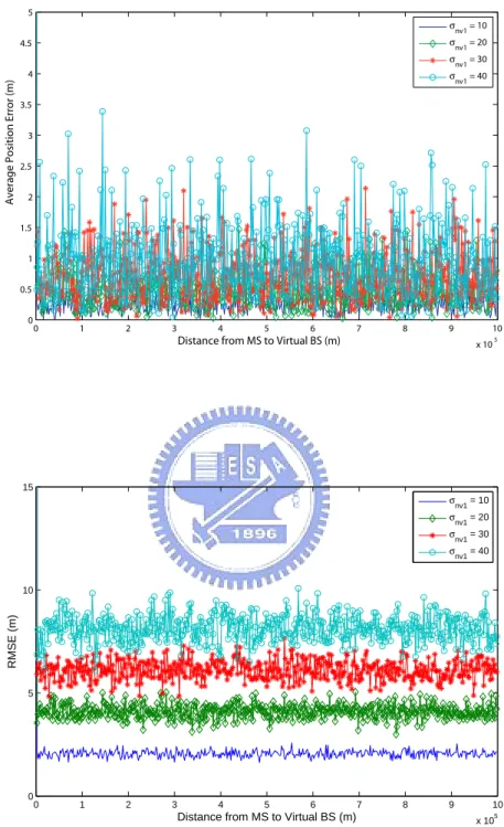
(43) from the measurement inputs as (i.e. ri,k = ζi,k + ni,k + ei,k in (2.1)) .  )2.  2ζ1,k (n1,k + e1,k ) + (n1,k + e1,k  2 ∆Jk =   2ζ2,k (n2,k + e2,k ) + (n2,k + e2,k )  2ζ3,k n3,k + n23,k. .   2ζ1,k (n1,k + e1,k )    '  2ζ (n + e ) 2,k   2,k 2,k   2ζ3,k n3,k.      . (5.13). where e3,k is considered zero as mentioned at the beginning of this proof. The approximation is valid by considering that the noiseless distance ζi,k is in general larger than the combined noise effect (ni,k +ei,k ). For simplicity and without lose of generality, coordinate transformation can be adopted within (5.12) such that (x1,k , y1,k ) = (0, 0). The expected value of the estimation error (i.e. ∆ˆ xk = [∆ˆ xk , ∆ˆ yk ]T ) can therefore be acquired by expanding (5.12) as ·. E[∆ˆ xk ] = = E[∆ˆ yk ] = =. ¸ ζ1,k (n1,k + e1,k )(y2,k − y3,k ) + ζ2,k (n2,k + e2,k )y3,k − ζ3,k n3,k y2,k E x3,k y2,k − x2,k y3,k ¸ · ζ1,k (n1,k + e1,k )(y2,k − y3,k ) + ζ2,k (n2,k + e2,k )y3,k (5.14) E x3,k y2,k − x2,k y3,k · ¸ ζ1,k (n1,k + e1,k )(x2,k − x3,k ) + ζ2,k (n2,k + e2,k )x3,k − ζ3,k n3,k x2,k E y3,k x2,k − y2,k x3,k · ¸ ζ1,k (n1,k + e1,k )(x2,k − x3,k ) + ζ2,k (n2,k + e2,k )x3,k E (5.15) y3,k x2,k − y2,k x3,k. It is noted that the second equalities for both (5.14) and (5.15) are attained based on the assumption that E[n3,k ] = 0. From (5.14) and (5.15), it can clearly be observed that the expected value of the estimation error (i.e. E[∆ˆ xk ] = [E[∆ˆ xk ], E[∆ˆ yk ]]T ) is independent to the measured distance r3,k under the assumption that its associated measurement noise n3,k is considered a zero mean random variable, i.e. E[r3,k ] = E[ζ3,k ] + E[n3,k ] = E[ζ3,k ]. This completes the proof. This lemma states that the expected value of the location estimation error is independent to the distance between a specific BS to the MS if the noises associated with the measurement inputs are statistically distributed with a zero mean value. In generic time-based location estimation, the phenomenon stated in Lemma 1 does not usually exist since most of the measurement inputs are contaminated with NLOS noises, i.e. ei,k in (2.1) is randomly distributed. 38.

(44) with positive mean value. The NLOS error is augmented as the distance between the specific BS and the MS is increased, which causes the corresponding measurement input to become unreliable comparing with the other signal sources. This result is consistent with the intuition that BSs with closer distances to the MS are always selected for location estimation. In the LT is considered as a designed distance proposed GPLT scheme, the virtual measurement rvGP 1 ,k. which is infected by its corresponding zero mean virtual noise nv1 ,k as in (4.10). Based on LT becomes uninfluential to the estimation error Lemma 1, the selection of the distance rvGP 1 ,k. while exploiting the WLS algorithm for location estimation. This result is similar to the derived GDOP value that is unrelated to the distance information between the BSs and the MS (as can be observed from (5.4)). In the simulation section, the uncorrelated relationship LT and the estimation error will further be validated by exploiting the two-step between rvGP 1 ,k. LS estimator, which is considered one of the the WLS-based algorithms for location estimation. It will be demonstrated via the simulation results that the influence from the length of the virtual measurement to the estimation error is considered insignificant. The procedures of the proposed GPLT scheme under the two-BSs case is explained as ˆ k|k ) based follows. The target is to obtain the position of the MS at the k th time step (i.e. x on the available information, including the measurement and location information acquired ˆk|k−1 ). Two from both BS1 and BS2 along with the predicted position of the MS (i.e. x steps are involved within the proposed GPLT scheme: (i) the determination of the virtual BS’s position and the virtual measurement; and (ii) the estimation and tracking of the MS’s position. As shown in Fig. 4.1, the orientation of the virtual BS (θkm ) relative to the the ˆk|k−1 is determined based on the criterion of minimizing the GDOP predicted MS’s position x ˆk|k−1 (as obtained from (5.5) and (5.6)). As was indicated by Lemma 1 in Subsection value on x LT w.r.t. the predicted MS’s position x ˆ k|k−1 V.A.(2), the selection of the virtual distance rvGP 1 ,k. is considered insignificant to the estimation errors. Therefore, the distance is selected the same LT = r P LT as in (4.5). The location of value as was designed in the PLT algorithm, i.e. rvGP v1 ,k 1 ,k GP LT LT the virtual BS (xGP v1 ,k ) and the length of the virtual measurement (rv1 ,k ) can consequently. be acquired. It is also noticed that the design of the virtual noise can therefore be selected. 39.

(45) the same as that in the PLT scheme, i.e. zero mean random distributed with variance σn2 v =. Var(rvP1LT ,k ). 1 ,k. = Var(kˆ x k|k−1 − xˆ k−1|k−1 k).. After acquiring the information of the virtual BS as the additional signal source, the exLT tended sets of the BSs and the measurement inputs can be established as PeBS,k = {x1,k , x2,k , xGP v1 ,k } LT }. As illustrated in Fig. 3.3, the extended set of signal sources are and rek = {r1,k , r2,k , rvGP 1 ,k. utilized as the inputs to the two-step LS estimator. The estimated MS’s position xˆ k|k can therefore be obtained by adopting the correcting phase of the Kalman filter, which completes the location estimation and tracking processes at the k th time step.. 5.3. The Single-BS Case. As illustrated in Fig. 4.2, only one BS (x1,k ) associated with the measurement input r1,k is available at the considered k th time instant. Additional two virtual BSs associated with their virtual measurements are required as the inputs for the two-step LS estimator, i.e. LT GP LT GP LT GP LT = {r GP LT , r GP LT }. By adopting the design from PGP BSv ,k = {xv1 ,k , xv2 ,k } and rv,k v1 ,k v2 ,k. the PLT scheme with the single-BS case, the first virtual BS is designed to be located at LT = x LT as defined in (4.5). ˆ k−1|k−1 associated with the first virtual measurement rvGP xGP v1 ,k 1 ,k LT is also designed to be the same as in the PLT The second virtual measurement rvGP 2 ,k. scheme (in (4.9)), which considers the averaged prediction error from the previous time steps. LT As shown in Fig. 4.2, the position of the second virtual BS (xGP v2 ,k ) is designed at a location LT relative to the predicted MS’s position x ˆ k|k−1 . The relative angle θkm bewith distance rvGP 2 ,k LT and x ˆ k|k−1 is determined by minimizing the GDOP value based on the predicted tween xGP v2 ,k. ˆ k|k−1 . Both of the information from BS1 and BSv1 alone with the predicted MS’s position x ˆ k|k−1 are utilized for the computation of the angle θkm (as in (5.5) and (5.6)). It MS’s position x is noticed that instead of altering the position of BSv1 , the BSv2 ’s location is adjusted in order ˆk|k−1 . The design concept is primarily to acquire a better GDOP value for the predicted MS x owing to the fact that the average prediction error is in general smaller than the length of LT > r GP LT . The expected each prediction within the Kalman filtering formulation, i.e. rvGP v2 ,k 1 ,k LT due to its smaller value comparing ˆk|k−1 is considered more sensitive to rvGP MS’s position x 2 ,k. 40.

(46) LT . It will be beneficial to adjust the location of BS (by rotating the angle with r1,k and rvGP v2 1 ,k. θkm ) such that a smaller GDOP value can be achieved at the predicted location of the MS (ˆ xk|k−1 ). LT is considered As indicated by Lemma 1, the selection of the virtual measurement rvGP 2 ,k LT is insignificant on the precision for location estimation. Nevertheless, the distance rvGP 2 ,k. chosen as in (4.9) in order to facilitate the design of the weighting coefficient associated with the two-step LS estimator. Similar to the design within the PLT scheme, the virtual noise LT can be regarded as zero mean with associated with the second virtual measurement rvGP 2 ,k. variance σn2 v. 2 ,k. LT ). Therefore, the information from the additional two virtual = Var(rvGP 2 ,k. LT and r GP LT can be acquired such as to provide sufficient signal sources measurements rvGP v2 ,k 1 ,k. for the two-step LS location estimator. The precision for location estimation and tracking of the MS can consequently be enhanced.. 41.

(47) Chapter 6. Performance Evaluation Simulations are performed to show the effectiveness of the proposed PLT and GPLT schemes under different numbers of BSs, including the scenarios with deficient signal sources. The noise models and the simulation parameters are illustrated in Subsection A. Subsection B validates the GPLT scheme according to the variations from the relative angle and the distance between the MS and the designed virtual BS. The performance comparison between the proposed PLT and GPLT algorithms with the other existing location tracking schemes, i.e. the Kalman Tracking (KT) and the Cascade Location Tracking (CLT) techniques, are conducted in Subsection C.. 6.1. The Noise Models and the Simulation Parameters. Different noise models [28] [47] for the the TOA measurements are considered in the simulations. The model for the measurement noise of the TOA signals is selected as the Gaussian distribution with zero mean and 10 meters of standard deviation, i.e. ni,k ∼ N (0, 100) . On the other hand, an exponential distribution pei,k (τ ) is assumed for the NLOS noise model of the TOA measurements as    pei,k (υ) =. 1. λi,k. ³ ´ exp − λυi,k υ>0.   0. otherwise. 42. (6.1).

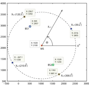
(48) 4000. 3500. o. Xv,1(120.5 ). X: 258.7 Y: 3392. X: 505 Y: 2957. o. 3000. Xv,1(30.2 ). rv,1. BS1. X: 2316 Y: 2855. 2500. θ. X: 1020 Y: 2100. 2000. 1500. 0. o. MS X: −267.1 Y: 1330. X: 1520 Y: 1234 o. BS2. Xv,1(210.9 ) 1000. X: 1781 Y: 807. 6. o. Xv,1(300.5 ) 500 −500. 0. 500. 1000. 1500. 2000. 2500. 3000. Figure 6.1: An Exemplify Diagram for the Scenarios with the Two-BSs Layout. Stars (xv,1 (30.2o ) and xv,1 (210.9o )): the Positions of the Virtual BS Cause the Minimal GDOP Value of the MS; Squares (xv,1 (120.5o ) and xv,1 (300.5o )): the Positions of the Virtual BS Cause the Maximal GDOP Value of the MS where λi,k = c · τi,k = c · τm (ζi,k )ε ρ. The parameter τi,k is the RMS delay spread between the ith BS to the MS. τm represents the median value of τi,k , which is selected as 0.1 in the simulations. ε is the path loss exponent which is assumed to be 0.5, and the factor for shadow fading ρ is set to 1 in the simulations. The parameters for the noise models as listed in this subsection primarily fulfill the environment while the MS is located within the rural area. It is noticed that the reason for selecting the rural area as the simulation scenario is due to its higher probability to suffer from deficiency of signal sources. Moreover, the sampling time ∆t is chosen as 1 sec in the simulations.. 6.2 6.2.1. Validation of the GPLT Scheme Validation with Angle Effect. As mentioned in Subsection V.A.(1), the primary objective of the proposed GPLT algorithm is to adjust the position of the virtual BS such that the predicted MS can be situated at a location. 43.

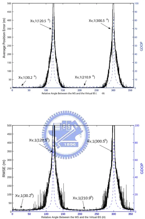
(49) 100. 450. 90. Xv,1(300.5 o). Xv,1(120.5 o). 400. 80. 350. 70. 300. 60. 250. 50. 200. 40. 150. 30. 100. GDOP. Average Position Error (m). 500. 20. o. o. Xv,1(210.9 ). Xv,1(30.2 ). 50. 10. 0. 0 0. 50. 100 150 200 250 Relative Angle Between the MS and the Virtual BS (. 300. 350. Θ). 500. 100. 450. o. Xv,1(300.5o). Xv,1(120.5 ). 400. 80. 300. 60. GDOP. RMSE (m). 350. 250 200. 40. 150. Xv,1(30.2o). 100. 20. Xv,1(210.9o). 50 0. 0. 50. 100 150 200 250 Relative Angle Between the MS and the Virtual BS (Θ). 300. 350. 0. Figure 6.2: Top Plot: the Average Position Error (Solid Line) and the GDOP Value (Dashed Line) vs the Relative Angle Between the MS and the Virtual BS (θ); Bottom Plot: the RMSE (Solid Line) and the GDOP Value (Dashed Line) vs the Relative Angle Between the MS and the Virtual BS (θ). 44.