台股風險值分析 - 政大學術集成

全文

(1)國立政治大學國際經營與貿易學系碩士論文. 台股風險值分析. 學. ‧ 國. Value at Risk 政 Based 治on Independent 大立 Component Analysis. ‧. n. er. io. sit. y. Nat. al. Ch. engchi. i n U. v. 指導教授：郭維裕博士 Advisor: Wei-Yu Kuo, Ph.D. 研究生: 曾順延 Shun-Yan Zeng 中華民國九十九年七月 July, 2010.

(2) Abstract……………………………………………………………………………………………………….…….2 1. Introduction ......................................................................................... 2. 2. Methodology ...................................................................................... 5 2.1.1 Independent component analysis.................................................. 5 2.1.2 Measures of nongaussianity ......................................................... 7. 政治大. 2.1.3 The FastICA Algorithm.................................................................. 8. 立. ‧ 國. 學. 2.2.1 Locally Adaptive Volatility Estimate ............................................. 9. ‧. 2.2.2 Applying additive error terms .................................................... 11. y. Nat. er. io. sit. 2.2.3. Adaptive estimation under local time homogeneity ................. 12. al. n. v i n C h................................................................ 2.3 GARCH and RiskMetrics 15 engchi U 2.4 Back-testing .................................................................................. 16 3. Empirical Study .................................................................................. 16 4. Conclusion ......................................................................................... 30. 5. Referance……………………………….………………………………………….…………….29 2.

(3) Abstract The Value at Risk (VaR) measures the potential loss in value of risky asset or portfolio over a defined period for a given confidence interval. The traditional way needs to estimate corresponding distribution and process of portfolio, which is very difficult. Independent component analysis (ICA) is designed for detection of blind folded signals and retrieves out of a high-dimensional time series stochastically independent source components. We can use the property of independence to. 政治大 estimate methods in conjunction 立 with independent component process to calculate. estimate distribution of portfolio easily. This paper uses three different volatility. ‧. ‧ 國. 學. value at risk.. 1. Introduction. sit. y. Nat. The study on risk management has been prompted by the Basel committee for. al. er. io. regular banking supervisory. It is used for risk control and management, including. v. n. both credit and operational risks (Duffee and Pan, 1997). The VaR is popular since. Ch. engchi. i n U. the 1996 amendments to the Basle Capital Accord incorporating market risk into the regulatory capital framework. Supervisory agencies allow banks to use their internal VaR models to calculate their regulatory capital requirements as an alternative to the conventional methodology. The systematic use of the VaR for different portfolios has had an overall positive effect on the handling of risk within financial institutions, matching the increasing degree of complexity of investment instruments over the last few years. Given a d-dimensional portfolio, the conditionally heteroscedastic model is widely used to describe the movement of the underlying series:. X t = σ tζ t 3.

(4) (1) Where X t ∈  d is the risk factor vector such as the log return of d individual financial instruments. The matrixes σ t denote the corresponding time-dependent covariance and ζ t the d-dimensional standardized residual vector. The portfolio VaR calculation becomes technically difficult for high dimensionality of the portfolio. The reason of difficulty is that it is hard to estimate covariance of relevant risk factors. Two issues are the distribution of portfolio and the underlying process of risk factors.. 政治大 RiskMetrics assume Gaussian 立 distributed residuals ε = Σ. The classical but not realistic approach is RiskMetrics launched by J.P. Morgan. −1/ 2. t. xt are independent. ‧ 國. 學. after devolatilization1 , so the distribution of portfolio is product of d marginals. Independent component analysis (Hyvärinen, 2001) is a feasible way to simplify the. ‧. calculation and more realistic than RiskMetrics. This engineering method is designed. y. Nat. sit. for detection of blind folded signals and retrieves out of a high-dimensional time. n. al. er. io. series stochastically independent source components. Using ICA to separate IC to. i n U. v. reconstruct risk factor process would increase accuracy of forecast (CHA and CHAN, 1. Ch. engchi. 2000), and easy to calculate VaR (Chen,2007). Beside RiskMetrics, another two volatility estimate are GARCH model and Locally Adaptive Volatility Estimate (Mercurio and Spokoiny, 2004, 2007) which are used to capture the risk factor process. It has better accuracy of VaR calculation which combines ICA and Locally Adaptive Volatility Estimate (LAVE) compared to single risk factor (Chen, 2007). This thesis calculates VaR of different distributions and volatility processes, but use slightly modified LAVE. By using modified LAVE and ICA, we get a better VaR model 1. * Devolatilization means data divided by its standard deviation.. 4.

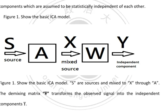
(5) than GARCH model and RiskMetrics model. Sections 2 introduces ICA and LAVE which are the fundamental methods in this thesis. We apply ICA and LAVE to calculate VaR by using Taiwan Indexes, and compare to GARCH and RiskMetrics in section 3. Finally, we conclude our study in Section 4. 2. Methodology 2.1.1 Independent component analysis. The ICA (see Comon, 1994 and Hyvärinen et al., 2001) is a statistical method that expresses a set of multidimensional observations as a combination of independent. 政治大 Figure 1. Show the basic ICA model. 立. components which are assumed to be statistically independent of each other.. ‧. ‧ 國. 學 er. io. sit. y. Nat. al. v. n. Figure 1. Show the basic ICA model. “S” are sources and mixed to “X” through “A”.. Ch. engchi. i n U. The demixing matrix “W” transforms the observed signal into the independent components Y. Below discuss figure 1 more explicit. When the function is linear, the simple model is: x = As. (2). Where A is an unknown (n xn) mixing matrix. The matrix X has observations x as its columns and similarly the matrix S has latent variable vectors s as its columns. The mixing matrix A is constant for all observations. The mixing process is hidden, so we can only observe the mixed signals. The independent components are latent 5.

(6) variables, meaning that they cannot be directly observed. The task is now to recover the original source signals from the observations through a demixing process. The following equations (3) and (4) mathematically describe the demixing processes: Y=WX. (3). Y=WAS. (4). and so:. Matrix S contains the original source signals driving the observations whereas the separated signals are stored in matrix Y. The (n xm) matrix W is the demixing matrix. If the separated signals are the same as the original sources (Y = S), the mixing matrix. 政治大 is the inverse of demixing matrix (A =W−1). 立. The key to estimating the ICA model is nongaussianity. According to central limit. ‧ 國. 學. theorem, the sum of a sufficiently large number of independent random variables,. ‧. each with finite mean and variance, will be approximately normally distributed. Thus,. y. Nat. a sum of two independent random variables usually has a distribution that is closer. er. io. sit. to gaussian than any of the two original random variables. The solution to ICA model is to maximize nongaussianity. This is because that according to central limit theorem. al. n. v i n and equation (4),”Y” has greaterCgaussianity than “S” U h e n g c h i unless Y=S.. To estimate one of. the independent components, we consider a linear combination of the xi ; let us denote this by Y = W T X , where w is a vector to be determined. If w were one of the rows of the inverse of A, this linear combination would actually equal one of the independent components. To estimate several independent components we need to calculate several wi .To prevent different vectors from converging to the same maxima we must decorrelate the outputs wT X 1 , , wT X n after every iteration. A simple way of achieving decorrelation is a deflation scheme based on a 6.

(7) Gram-Schmidt-like decorrelation. This means that we estimate the independent components one by one. When we have estimated p independent components or p p. wp +1 − ∑ ( wpT +1wi )wi . vectors w1 , , wp , we calculate wp +1 and orthonormalized w= p +1 i =1. 2.1.2 Measures of nongaussianity The classical measure of nongaussianity is kurtosis. The kurtosis of y is classically defined by. ku= tr( y ) E ( y 4 ) − 3E ( y 2 ) 2. (5). 政治大. We assumed that y is of unit variance, and the right-hand side simplifies to. 立. E ( y 4 ) − 3 . For a Gaussian y, the fourth moment equals 3E ( y 2 ) 2 . Thus, kurtosis is. ‧ 國. 學. zero for a Gaussian random variable. Nongaussianity is measured by the absolute. ‧. value of kurtosis, because kurtosis might be positive or negative. No matter positive. y. Nat. or negative, the greater absolute value means far from Gaussian.. er. io. sit. Another very important measure of nongaussianity is given by negentropy. Negentropy is based on the information theoretic quantity of entropy. The entropy. al. n. v i n of a random variable can be C interpreted as the degree h e n g c h i U of information that the. observation of the variable gives. The larger entropy means more randomness of a variable. Entropy H is defined for a discrete random variable Y as H ( y) = −∑ P(Y = ai ) lo P (Y g= ai ). (6). Where ai are the possible values of Y and P is probability of Y= ai . The definition is for discrete random variables and vector. The differential entropy (continue) H of a random vector y with density f (y) is defined as (Cover and Thomas, 1991; Papoulis, 1991) 7.

(8) H ( y ) = − ∫ f ( y ) lo gf ( y )d y. (7). A fundamental result of information theory is that a Gaussian variable has the largest entropy among all random variables of equal variance. This shows that the Gaussian distribution is the “most random” or the least structured of all distributions. We can use this property to measure non-gaussianity. In order to obtain a measure of non-gaussianity, one often uses a slightly modified version of the definition of differential entropy, called negentropy. Negentropy J is defined as follows. 政治大. = J ( y ) H ( y( gauss ) ) − H ( y ). 立. (8). Due to the above-mentioned properties, negentropy is always non-negative, and it. ‧ 國. 學. is zero if and only if y has a Gaussian distribution. The advantage of using negentropy as a measure of nongaussianity is well justified by statistical theory. Estimating. ‧. negentropy using the definition would require an estimate of the pdf, what is very. y. Nat. sit. difficult to compute. It’s difficult to estimate the negentropy as mention above.. n. al. er. io. In practice, some approximations have to be used. The classical method of. i n U. approximating negentropy is using higher-order moments:. Ch. J ( y) ≈. engchi. v. 1 1 E[ y 3 ]2 + kurt ( y ) 2 12 48. (9). The random variable y is assumed to be of zero mean and unit variance, but these approximations suffer from the non-robustness encountered with kurtosis, because outlier has great influence on kurtosis. To avoid the problems encountered with the preceding approximations of negentropy, new approximations were developed in (Hyvärinen, 1998b). These approximations were based on the maximum-entropy principle. In general we obtain the following approximation: p. J ( y ) ≈ ∑ ki [ E{Gi ( y )} −E{Gi (v)]2 i =1. 8. (10).

(9) where ki are some positive constants. The variable y is assumed to be of zero mean and unit variance, and the functions Gi are some nonquadratic functions (Hyvärinen, 1998b). Although it is not accurate, it is consistent. In the case where we use only one nonquadratic function G, the approximation becomes. J ( y ) ∝ [ E{G ( y )} − E{G (v)}]2. (11). In particular, choosing G that does not grow too fast, one obtains more robust estimators. The following choices of G have proved very useful (Hyvärinen, 1998): 1 log cosh a1u a1. 政治大 − exp(−u / 2) 立G (u) = G1 (u ) =. (12). 2. 2. ‧. ‧ 國. 學. 1 ≤ a1 ≤ 2 is some suitable constant.. Where. 2.1.3 The FastICA Algorithm. io. the nongaussianity of W T X (Hyvärinen, 1999).. n. al. er. sit. y. Nat. The FastICA is based on a fixed-point iteration scheme for finding a maximum of. i n U. v. 1. Choose an initial vector wi of unit norm, W = ( w1 ,..., wd )T. = E{g ( w 2. Let w (n) j. ( n −1) j. Ch. x) x} − E ( g '( w. engchi. ( n −1) j. x)}w(jn −1) , where g denotes the first derivative. of and g’ the second derivative. In practice, the sample mean is applied for E[.] (n) w(jn ) − ∑ ( w(jn ) wk )wk 3. Orthogonalization w= j T. k≠ j. (n) (n) (n) 4. Normalization w j = w j / || w j || (n) ( n −1) 5. If not converged, || w j − w j ||≠ 0 go back to step 2.. 6. Set j=j+1. For j ≤ d , d=number of risk factors, go back to step 2.. 9.

(10) 2.2.1 Locally Adaptive Volatility Estimate The FastICA algorithm separates the independent components. It’s impotent to capture the process of independent components when forecast value at risk. The estimator of volatility play a critical role when capture the process. Locally Adaptive. 政治大 any parametric form of the volatility process. It just assumes the volatility can be 立 Volatility Estimate developed by Mercurio and Spokoiny (2004). It does not assume. finding the interval which is homogeneity.. 學. ‧ 國. approximated by a constant over some interval. Therefore, the main problem is. ‧. With the LAVE approach the model is regularly checked and adapted to the data,. y. Nat. meaning that for every time point t we estimate the past interval of time. er. io. sit. homogeneity [t − τ , t], over which the volatility is nearly constant. LAVE gives a test procedure which discuss in 2.2.3. Once this interval is defined, we estimate the. al. n. v i n C h ahead forecastingU(since the volatility process is corresponding volatility by one-step engchi a supermartingale) and the volatility is estimated by the past squared returns. For example, assume the underlying process is classical modeled as conditional heteroscedastic by:. Rt = σ tζ t. (13). Where, ζ t is a sequence of independent standard Gaussian random variable. The. σ t is volatility process which can be estimate by past information. For every time point t, we can fine an interval of time homogeneity [t − τ , t]. LAVE assume volatility. 10.

(11) of the interval [t − τ , t] is constant, so the local constant volatility σ τ can be estimate by averaging the past squared returns Rt 2 for t ∈ I (I= interval of time homogeneity) ^. 2. στ =. 1 Rt 2 ∑ | I | t∈I. (14). 2.2.2 Applying additive error terms We can find a new setting of model unlike former discuss to apply LAVE easily. The. 政治大 to a regression with additive noise and much closer to a Gaussian one. Due to 立 approach is the power transformation [see Carroll and Ruppert (1988)] which leads. ‧ 國. 學. Rt = σ tζ t , the random variable Rt is conditionally on Ft −1 Gaussian and. E ( Rt2 | Ft −1 ) = σ t2. (15). ‧. Similarly, for every γ > 0. sit. y. Nat. n. al. er. io. γ γ E (| Rt |γ | Ft −1 ) σ= Cγ σ tγ = t E (| ζ | | Ft −1 ). Ch. n U engchi. iv. 2 = σ t2γ Dγ2 E (| Rt |γ −Cγ σ tγ | = Ft −1 ) σ t2γ E (| ζ |γ −C γ). where ζ. (16) (17). denotes a standard Gaussian r.v., Cγ = E (| ζ |γ ) and Dγ2 = Var. | ζ |γ .Therefore, the process | Rt |γ allows for the representation. | Rt |γ = Cγ σ tγ + σ tγ Dγ ς t. (18). Where ς t is equal to (| ζ |γ −Cγ ) / Dγ . Note that the problem of estimating σ t is in some sense equivalent to the problem of estimating θt = Cγ σ tγ which is the conditional mean of the transformed process | Rt | . This is already a kind of 11.

(12) heteroscedastic regression problem with additive errors σ tγ Dγ ς t satisfying. E (σ tγ Dγ ς t | Ft −1 ) = 0 E (σ t2γ Dγ2ς t2 | Ft −1 ) = σ t2γ Dγ2. (19). LAVE want to justify the interval of time homogeneity. It is more convenient to construct a test procedure with equation (18) than equation (13), because the equation (18) turns error term from multiplicative one to additive one.. 政治大. 2.2.3. Adaptive estimation under local time homogeneity. 立. The assumption of local time homogeneity means that the function σ t is nearly. ‧ 國. 學. constant within an interval I= [t − τ , t], and the process Rt follows the regression. ‧. like equation (18) with the constant trend θt = Cγ σ tγ which can be estimated by. y. n. al. Ch. sit. io. ~. θI =. 1 | Rt |γ ∑ | I | t∈I. er. Nat. averaging over this interval I:. engchi U ~. (20). v ni. Below discuss the property of estimator θ I . According to equation (16), equation (18) and equation (20): ~. = θI. Cγ. D. σ γ + γ ∑σ γ ς ∑ |I| |I| t∈I. =. t. t∈I. t. t. divided by Cγ. (21). S 1 θt + γ ∑ θtς t ∑ | I | t∈I | I | t∈I. (22). Where Sγ = Dγ / Cγ , so that ~. E θ I =E(. 1 ∑ θt ) | I | t∈I. ~. (23) ~. θ I is an unbiased estimator in homogenous interval, and the variance of θ I is 12.

(13) Sγ2 | I |2. E (∑ θ t ς t ) = 2. t∈I. Sγ2 | I |2. E ∑ θt2. (24). t∈I. Equation (24) is applied to construct the test procedure. Due to our assumption of local homogeneity, the process θt is close to θτ for all t∈I. Define also = ∆ I sup | θt − θτ | and ν = 2 I. t∈I. S 2γ. ∑θ |I| t∈I. 2 t. (25). The value of ∆ I measures the departure from homogeneity within the interval I, and ~. it can be regarded as an upper bound of the “bias” of the estimate θ I . The value of. ν I2. 政治大 will be referred as the 立 “conditional variance” of the estimate θ ~. I. .. ‧ 國. 學. Given observations R1 , , Rn following the time-inhomogeneous model (18), we ~. ‧. aim to estimate the current value of the parameter θτ using the estimate θ I with. y. Nat. a properly selected time interval I of the form I= [t − τ , t] to minimize the. er. io. sit. corresponding estimation error. Below we discuss one approach which goes back to the idea of pointwise adaptive estimation; see Lepski (1990), Lepski and Spokoiny. al. n. v i n C hidea of the methodU can be explained as follows. (1997) and Spokoiny (1998). The engchi. Suppose I is an interval candidate; that is, we expect time homogeneity in I and, hence, in every subinterval of I. This implies that the value ∆ I is small and similarly for all ∆ J , J ⊂ I, and that the mean values of the θt over I and over J nearly coincide. This adaptive procedure roughly means the choice of the largest possible. interval I such that the hypothesis that the value θt is a constant within I is not rejected. For testing this hypothesis, Spokoiny suggest to consider the family of subintervals of I of the form J= [τ − m ',τ ] with m’< m and for every such subinterval J compare two different estimates: one is based on the observations from 13.

(14) J, and the other one is calculated from the complement I \ J = [τ − m,τ − m '] . Theorem to justify homogenous interval has been proofed by Spokoiny (2004). His defined below: ~. ~. ~. ~. | θ I \ J − θ J |> λ ( ν I \ J 2 + ν J 2 ). (26) ~. ~. Therefore, if there exists a testing interval J ⊂ I such that the quantity | θ I \ J − θ J | is. significantly positive, then we reject the hypothesis of homogeneity for the interval. The test procedure starts from an initial small interval I that satisfies the homogeneity and consists of 4 steps (Mercurio and Spokoiny (2004)):. 立. 政治大. Step 1: Enlarge the interval I from [τ − m0 ,τ ] to [τ − K * m0 ,τ ] , i.e. m = k* m0 ,and. ‧ 國. 學. split the new interval into two subintervals J and I\J. The parameters m0. ‧. and k are integers specified according to data. In this paper, we chose m0 =. al. er. io. sit. y. Nat. 5 and k= 2.. v. n. 2 Step 2: Start homogeneity test for interval J = [τ − m ,τ ] . If the homogeneity 3. Ch. engchi. i n U. 2 hypothesis isn’t rejected, enlarge J one point further to [τ − m − 1,τ ] and 3. repeat the homogeneity test. The choice of 1/3 comes from the fact that the right 1/3 part has been tested in the last homogeneous interval and the left one-thirds will be tested in the next homogeneous interval, Mercurio and Spokoiny (2004).. Step 3: If (14) is violated at point s, the loop stops and the time homogeneous interval I is specified from point τ to point s + 1.. 14.

(15) Step 4: If time homogeneity holds for this interval, go back to Step 1.. This thesis has slightly modified this procedure which doesn’t use 1/3m to avoid repeating testing. According to above test procedure, the condition is only used to justify the homogeneous interval, but “adaptive” means the rapid reflect of volatility. It is more important to reflect quickly than avoid repeating, because volatility cluster is common pattern in financial data. When a new point (forecasting) has important influence on homogeneity, we must apply a new homogeneous interval quickly, so this thesis test every point in I when forecasting. The largest interval I is finally. 政治大 chosen as the time homogeneous interval for point τ and local volatility σ 立. is. ‧. ‧ 國. 學. estimated.. t. 2.3 GARCH and RiskMetrics. sit. y. Nat. Unlike locally adaptive volatility estimate, GARCH is a traditional way to estimate. n. al. er. io. heteroscedastic volatility which developed by Bollerslev in 1986. The GARCH (p, q). v. 2 model (where p is the order of the GARCH terms σ and q is the order of the ARCH. terms ε ) is given by 2. Ch. i n U. engchi. q. p. σ 2t = α 0 + α1ε t2−1 + ..... + α qε t2− q + β1σ 2t −1 + ..... + β pσ 2t − p = α 0 + ∑ α iε t2−i + ∑ βiσ 2t −i =i 1 =i 1. (27). The estimator of volatility is according to assumption of distribution by using MLE. The RiskMetrics variance model (also known as exponential smoother) was first established in 1989 by J.P Morgan. 2 σ= λσ t2−1 + (1 − λ )rt 2−1 t. (28). The optimal (theoretical) lambda varies by asset class, but the overall optimal parameter used by RiskMetrics has been 0.94. In practice, RiskMetrics only uses one 15.

(16) decay factor for all series: 0.94 for daily data and 0.97 for monthly data (month defined as 25 trading days). 2.4 Back-testing Backtesting (or back-testing) is the process of evaluating a strategy, theory, or model by applying it to historical data. A key element of backtesting that differentiates it from other forms of historical testing is that backtesting calculates how a strategy would have performed if it had actually been applied in the past.. 政治大 however a high or successful correlation between a backtested strategy and 立. Backtesting is a common and methodologically accepted approach to research,. historical results can never prove a theory correct, since past results do not. ‧ 國. 學. necessarily indicate future results. Varieties of tests have been proposed to gauge the. ‧. accuracy of a VaR model. Some of the earliest proposed VaR backtests, e.g. Kupiec. y. Nat. (1995), focused exclusively on the property of unconditional coverage. In short, these. er. io. sit. tests are concerned with whether or not the reported VaR is violated more than α % of the time. He assumes failure rate (n/T) is binomial distribution.. n. al. Ch. i n U. v. T  P(= n, α , T )   p n (1 − P)T − n n. engchi. (29). The hypnosis is H 0 : α = (n / T ) and LR test is. LR = −2 ln[(1 − α )T − n α n ] + 2 ln[(1 − n / T )T − n (n / T ) n ]. (30). If LR > χ 2 (1 − α ,1) reject H 0 , means the VaR model “might” not be a good model. 3. Empirical Study In this section, this thesis uses two Taiwan stock index as for electronic and financial industries in Taiwan to calculate value at risk by RiskMetrics, GARCH (1, 1) and LAVE. When calculate value at risk of the portfolio, the proportion of each index 16.

(17) is identical during time. Because the proportion is time-invariant, the distribution of the portfolio can be estimated by Monte Carlo simulation. The time period of data is from 2000/05/19 to 2010/05/18, each index has 2496 observations. First 1496 observations are used to estimate RiskMetrics and GARCH model parameter, the other are used to forecast volatility (LAVE does not specify the parameters). Apply the FastICA algorithm to extract two independent components from two indexes. We want to compare VaR with different models, so each independent component use three different volatility estimators and two residual distributions to. 政治大. estimate the process. The demixing matrix W is:. 立. (31). ‧. ‧ 國. 學.  09766 −1.61416  1.8302 −0.5704   . sit. y. Nat. According to equation (3), we can use W2×2 multiplied by X 2×2496 (original data). n. al. er. io. to get two independent components S 2×2496 . Table 1 shows statistical property of. i n U. v. original index and estimated independent components. All the statistical property of. Ch. engchi. data is slight right-skewed and leptokurtic which are common in financial data. Before we fit the each IC of GARCH (1,1) and RiskMetrics with different distribution, we calculate volatility of LAVE first. This is because LAVE has different interval of homogeneity periods at different points, we must use the same period in GARCH (1,1) and RiskMetrics to compare. We use the equation (26) to test IC1 and IC2 from 600 to 2496. LAVE need enough past observations to apply testing. Our goal is to forecast from 1497 to 2496, so it is not important to choose the start point when used LAVE. We apply LAVE, where λ =1.06 and γ =0.5 which are suggested by Mercurio and Spokoiny (2004), to IC1 and IC2. Once we know the interval of homogeneity, we can 17.

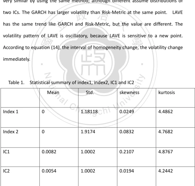
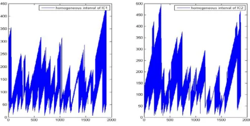
(18) use equation (14) to calculate corresponding volatility. Figure 1 shows the corresponding homogeneous interval of IC1 and IC2. The average homogeneous interval of IC1 (IC2) is 125.66(154.93), these values are used by GARCH and RiskMetrics when forecasting. Now we use first 1496 observations to estimate the parameter of GARCH and RiskMetrics. Table 2 presents the corresponding coefficient of independent component by GARCH (coefficient of RiskMetrics is λ =0.94). Figure 2 and 3 shows the corresponding volatility process of each IC. The volatility process is very similar by using the same method; although different assume distributions of. 政治大 has the same trend like GARCH and Risk-Metric, but the value are different. The 立. two ICs. The GARCH has larger volatility than Risk-Metric at the same point. LAVE. volatility pattern of LAVE is oscillatory, because LAVE is sensitive to a new point.. ‧ 國. 學. According to equation (14), the interval of homogeneity change, the volatility change. ‧. immediately.. y. Nat. n. al. Std.. Index 1. 0. Index 2. 0. IC1 IC2. Table 1.. Ch. engchi. 1.18118. skewness. er. io. Mean. sit. Table 1. Statistical summary of index1, index2, IC1 and IC2. i n U. v. kurtosis. 0.0249. 4.4862. 1.9174. 0.0832. 4.7682. 0.0082. 1.0002. 0.2107. 4.8767. 0.0054. 1.0002. 0.0194. 4.2442. Statistical summary of index1, index2, IC1 and IC2. All the statistical. property of data is slight right-skewed and leptokurtic which are common in financial 18.

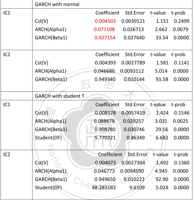
(19) data. Table 2. Corresponding coefficient of independent component by GARCH GARCH with normal IC1 Cst(V) ARCH(Alpha1) GARCH(Beta1). Coefficient Std.Error t-value t-prob 0.004503 0.0039121 1.151 0.2499 0.071108 0.026713 2.662 0.0079 0.927154 0.027640 33.54 0.0000. Cst(V) ARCH(Alpha1) GARCH(Beta1). Coefficient Std.Error t-value t-prob 0.004393 0.0027789 1.581 0.1141 0.046686 0.0093112 5.014 0.0000 0.949340 0.010144 93.58 0.0000. IC2. y. Nat. n. al. sit. io. Cst(V) ARCH(Alpha1) GARCH(Beta1) Student(DF). Coefficient Std.Error 0.004073 0.0027304 0.046773 0.0094590 0.949650 0.010222 48.283183 9.6109. er. IC2. 0.008178 0.088678 0.908780 5.770221. ‧. Cst(V) ARCH(Alpha1) GARCH(Beta1) Student(DF). t-value 0.0057419 1.424 0.029257 3.031 0.030746 29.56 0.86349 6.682. 學. ‧ 國. IC1. 政治大 GARCH with student T 立 Coefficient Std.Error. Ch. engchi. i n U. v. t-value 1.492 4.945 92.90 5.024. t-prob 0.1546 0.0025 0.0000 0.0000 t-prob 0.1360 0.0000 0.0000 0.0000. Table 2. Corresponding coefficient of independent component by GARCH. According to equation (27), the variance equation of IC1 with normal distribution is 2 σ 2t = 0.004503 + 0.927154σ 2t −1 + 0.071108ε t-1. Figure 1. Homogeneous interval of IC1 and IC2. 19.

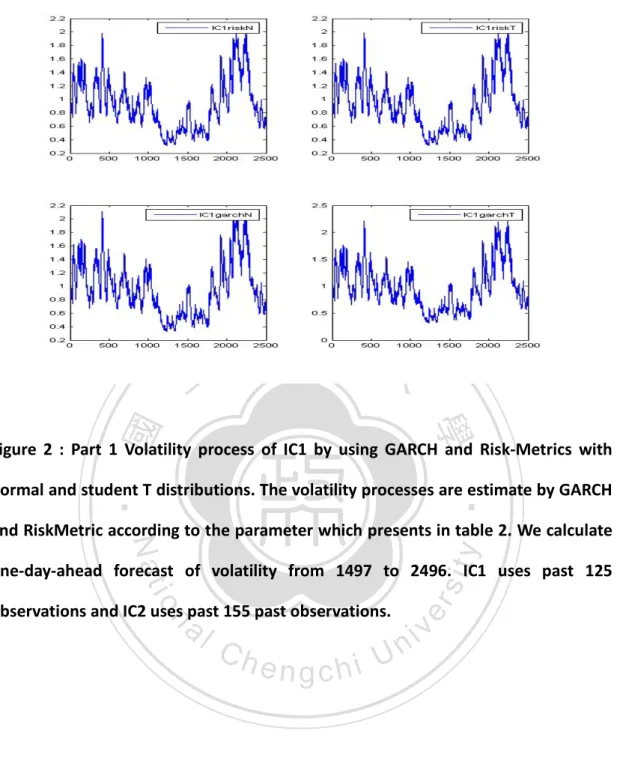
(20) Figure 1. Homogeneous interval of IC1 and IC2.These interval are estimated by ~. ~. ~. | θ I \ J − θ J |> λ ( ν I \ J + 2. 治政 1 ν ) , and used to calculate σ大= ∑R |I| 立 ~. 2. ^. 2. τ. J. t∈I. 2. t. . The pattern of. ‧ 國. 學. homogeneous interval is oscillatory, because LAVE estimate volatility at every point, and sensitive to a new point.. ‧ er. io. sit. y. Nat. al. v. n. Figure 2 : Part 1 Volatility process of IC1 by using GARCH and Risk-Metrics with. Ch. normal and student T distributions.. engchi. 20. i n U.

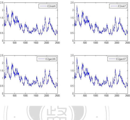
(21) 立. 政治大. ‧ 國. 學. Figure 2 : Part 1 Volatility process of IC1 by using GARCH and Risk-Metrics with. ‧. normal and student T distributions. The volatility processes are estimate by GARCH. y. Nat. and RiskMetric according to the parameter which presents in table 2. We calculate. observations and IC2 uses past 155 past observations.. n. al. Ch. engchi. er. io. sit. one-day-ahead forecast of volatility from 1497 to 2496. IC1 uses past 125. i n U. v. Figure 2 : Part 2 Volatility process of IC2 by using GARCH and Risk-Metrics with normal and student T distributions. 21.

(22) 立. 政治大. ‧. ‧ 國. 學 y. Nat. Figure 2 : Part 2 Volatility process of IC2 by using GARCH and Risk-Metrics with. er. io. sit. normal and student T distributions. The volatility processes are estimate by GARCH and RiskMetric according to the parameter which presents in table 2. We calculate. n. al. one-day-ahead forecast of. v i n C h from 1496 Uto 2495. volatility engchi. observations and IC2 uses past 155 past observations.. Figure 3: Part 1 Volatility process of IC1 by using LAVE. 22. IC1 uses past 125.

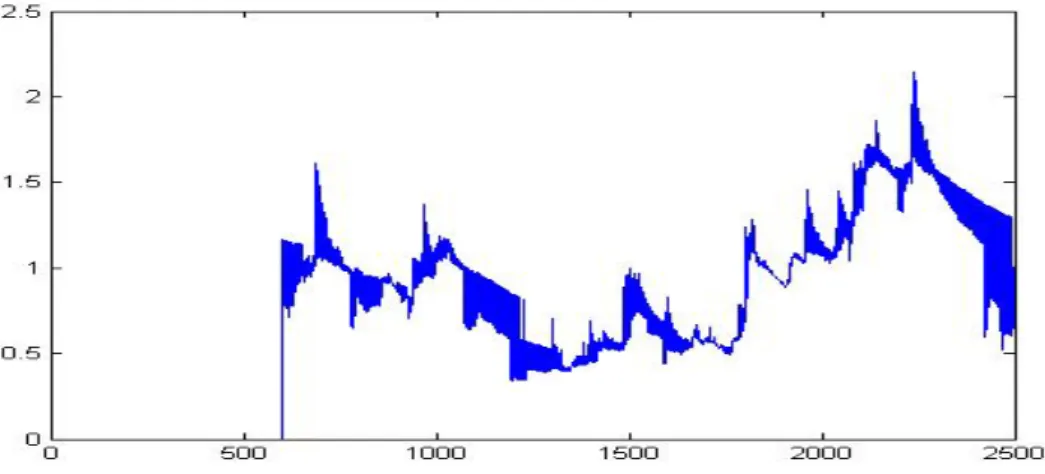
(23) Figure 3: Part 1 Volatility process of IC1 by using LAVE. According to homogeneous ^. 治 by σ 政 volatility interval at every point, we calculate 大立 point. vertical line which is the beginning. 2. τ. =. 1 Rt 2 ∑ | I | t∈I . There is a. ‧ 國. 學. Figure 3: Part 2 Volatility process of IC2 by using LAVE. ‧. n. er. io. sit. y. Nat. al. Ch. engchi. i n U. v. Figure 3: Part 2 Volatility process of IC2 by using LAVE. According to homogeneous ^. interval at every point, we calculate volatility by. 2. στ =. 1 ∑ Rt 2 | I | t∈I . There is a. vertical line which is the beginning point. The keys to evaluate VaR are volatility and quantile function, so the distribution of 23.

(24) portfolio is important. The independent distributions are assumed ‘T’ and ‘Normal’, and it’s possible to find the combination of distribution. The Monte Carlo is a feasible method to estimate the quantile function. We know that R = bX. (32). Where R is return of portfolio, b is proportion of each index, X=return of index. According to equation (3) and (13), we can represent (32) as. Ri = bAσ iε i. (33). Where R is return of portfolio, b is proportion of each index (equal in this thesis), A. 政治大. is mixing matrix, σ i is decided by GARCH, RiskMetrics, or LAVE. ε i is a normal or T. 立. distribution. This thesis generate d=2 samples, M=10000 observations, repeat 100. ‧ 國. 學. times and forecast 1000 days to calculate value at risk of portfolio. We illustrate this Monte Carlo simulation more explicit. For day 1497, we generate 10000 observations. ‧. from normal or T distribution, and calculate equation (33) which b, A, and σ i are. y. Nat. er. io. sit. already known, then we can get the simulative distribution of R to calculate the VaR. We repeat 100 times, and average the VaR. This is VaR at 1497, and we redo the. n. al. steps for the other 999 days.. v i n C Figure 4, 5, 6 shows the h e n g c h i U simulation of value at risk at. different alpha. The failure number means the numbers of original return lower than. forecasted VaR. The failure number of GARCH with T is 9, GARCH with normal is 32, RiskMetrics with T is 15, RiskMetrics with normal is 31, LAVE with T is 6, and LAVE with normal is 21 at alpha=0.01. The failure number of GARCH with T is 6, GARCH with normal is 18, RiskMetrics with T is 7, RiskMetrics with normal is 22, LAVE with T is 4, and LAVE with normal is 14 at alpha=0.005. The failure number of GARCH with T is 2, GARCH with normal is 12, RiskMetrics with T is 6, RiskMetrics with normal is 13, LAVE with T is 1, and LAVE with normal is 8 at alpha=0.0025. All the failure number is used to backtesting. Table 3 presents the result of simulation for alpha=0.01 with 24.

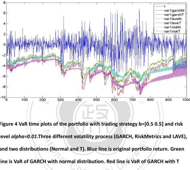
(25) different model and distributions. Figure 4 One-day-ahead forecast VaR for 1000 days. Alpha=0.01.. 立. 政治大. ‧. ‧ 國. 學. Figure 4 VaR time plots of the portfolio with trading strategy b=[0.5 0.5] and risk. y. Nat. sit. level alpha=0.01.Three different volatility process (GARCH, RiskMetrics and LAVE),. n. al. er. io. and two distributions (Normal and T). Blue line is original portfolio return. Green. i n U. v. line is VaR of GARCH with normal distribution. Red line is VaR of GARCH with T. Ch. engchi. distribution. Indigo line is VaR of LAVE with normal distribution. Pink line is VaR of LAVE with T distribution. Khaki line is VaR of RiskMetrics with normal distribution. Gray line is VaR of RiskMetrics with T distribution. The failure number of GARCH with T is 9, GARCH with normal is 32, RiskMetrics with T is 15, RiskMetrics with normal is 31, LAVE with T is 6, and LAVE with normal is 21. 25.

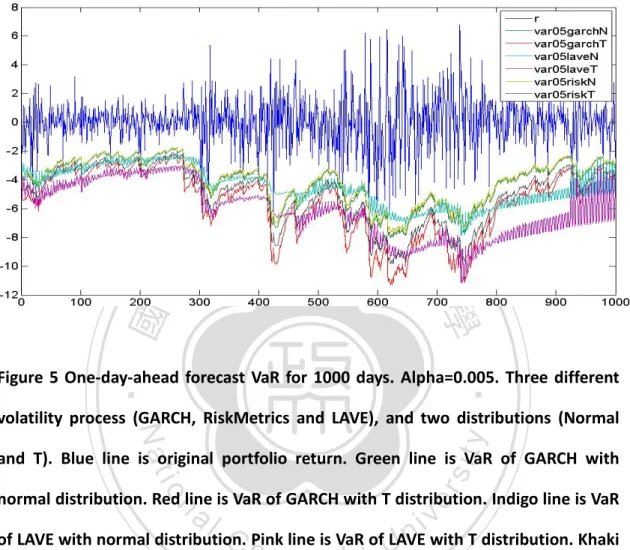
(26) Figure 5 One-day-ahead forecast VaR for 1000 days. Alpha=0.005. 立. 政治大. ‧ 國. 學 ‧. Figure 5 One-day-ahead forecast VaR for 1000 days. Alpha=0.005. Three different. y. Nat. volatility process (GARCH, RiskMetrics and LAVE), and two distributions (Normal. er. io. sit. and T). Blue line is original portfolio return. Green line is VaR of GARCH with normal distribution. Red line is VaR of GARCH with T distribution. Indigo line is VaR. al. n. v i n C hPink line is VaR ofULAVE with T distribution. Khaki of LAVE with normal distribution. engchi. line is VaR of RiskMetrics with normal distribution. Gray line is VaR of RiskMetrics with T distribution. The failure number of GARCH with T is 6, GARCH with normal is 18, RiskMetrics with T is 7, RiskMetrics with normal is 22, LAVE with T is 4, and LAVE with normal is 14 at alpha=0.005. 26.

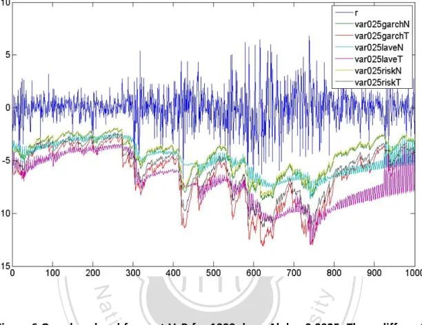
(27) Figure 6 One-day-ahead forecast VaR for 1000 days. Alpha=0.0025.. 立. 政治大. ‧. ‧ 國. 學 sit. y. Nat. n. al. er. io. Figure 6 One-day-ahead forecast VaR for 1000 days. Alpha=0.0025. Three different. i n U. v. volatility process (GARCH, RiskMetrics and LAVE), and two distributions (Normal. Ch. engchi. and T). Blue line is original portfolio return. Green line is VaR of GARCH with normal distribution. Red line is VaR of GARCH with T distribution. Indigo line is VaR of LAVE with normal distribution. Pink line is VaR of LAVE with T distribution. Khaki line is VaR of RiskMetrics with normal distribution. Gray line is VaR of RiskMetrics with T distribution. The failure number of GARCH with T is 2, GARCH with normal is 12, RiskMetrics with T is 6, RiskMetrics with normal is 13, LAVE with T is 1, and LAVE with normal is 8 at alpha=0.0025.. 27.

(28) Table 3: The value of simulation of each model at alpha=0.01. Risk-Metrics(N). 437 438 439 998 999 1000. 0.054434 0.052317 0.054613 ⁞ 0.082051 0.086927 0.090703 ⁞ 0.041887 0.040148 0.042671. 1 2 3. -3.94597 -3.94938 -4.10851 ⁞ 460 -4.77862 461 -5.73632 462 -5.70821 ⁞ 998 -3.30006 999 -3.21958 1000 -3.33102. 立. 306 307 308. 1000. ‧ 國. 1 2 3. -2.61847 -3.4173 -2.58854 ⁞ 475 -4.40064 476 -4.39695 477 -4.38209 ⁞ 998 -4.1552 999 -2.66425 1000 -2.4732. al. Ch. std 0.037363 0.045978 0.04415 ⁞ 0.085569 0.074855 0.060715 ⁞ 0.064084 0.045015 0.041902. engchi. std. -3.40822 -3.42196 -3.55315 ⁞ -4.25849 -4.24044 -4.16109 ⁞ -2.85039 -2.76901 -2.87676. 0.05615 0.054582 0.057865 ⁞ 0.06655 0.068768 0.063831 ⁞ 0.046785 0.041473 0.046473. 1 2 3. 471 472 473. i n U. LAVE(T). Mean. std. -3.32026 -4.46174 -3.25685 ⁞ -5.68573 -5.60884 -5.64054 ⁞ -5.59722 -3.45916 -3.19784. 0.070374 0.098782 0.072394 ⁞ 0.11883 0.107115 0.124786 ⁞ 0.147072 0.077983 0.072974. ‧. 0.091322 0.095837 0.115051 ⁞ 0.116788 0.109204 0.108098 ⁞ 0.085506 0.081037 0.077226. Mean. 學. Mean. n. 998 999 1000. std. io. 455 467 457. -4.47324 -4.43185 -4.65819 ⁞ -5.4265 -5.34339 -5.19116 ⁞ -3.68396 -3.58191 -3.69437. 1 2 3. LAVE(N). Nat. 1 2 3. 0.089946 0.091944 0.085457 ⁞ 0.129563 0.144323 0.133203 ⁞ 0.062374 0.068691 0.071665. 998 政治大 999. GARCH(T) Mean. std. y. -3.248 -3.27626 -3.38771 ⁞ -5.78364 -5.65688 -5.51541 ⁞ -2.74154 -2.65891 -2.76765. Mean. sit. 1 2 3. std. GARCH(N). er. Mean. Risk-Metrics(T). v. 998 999 1000. Table 3: The value of simulation of each model at alpha=0.01. For example, mean of VaR of Risk-Metrics with normal distribution for day 1 is -3.248.. Back-testing result of each type model is presents in table 4. The failure rate (n/T) means failure numbers divided by total days of forecast. According to equation (33), we can calculate the value of LR test. The critical value of LR test for alpha=0.01 is 28.

(29) 6.63, alpha=0.005 is 7.88, and alpha=0.0025 is 9.14. The star sign is LR test value over critical value. Apparently, normal distribution is not a suitable distribution, no matter what volatility estimator use, the failure rate of given alpha are higher than student t distribution. Locally adaptive volatility estimate may a good estimator which has fewer stars than Risk-Metrics and GARCH by given distribution.. Table 4. Back-testing result of each type model Risk-Metrics(N) Alpha 0.01. x/T. Risk-Metrics(T). LR. 0.031. 28.5956. 立. GARCH(N). x/T LR 政治大 0.015 2.1892. x/T. LR. 0.032. 30.9342. 0.01. 0.009. 0.006. 0.018. 3.5179. 28.2865 ＊. 0.012. 18.7375. y. 21.9760. LR. er. al. ＊. sit. ＊ LAVE(N). n. x/T. 0.7146. ＊. io. GARCH(T). 0.007. ‧. 0.013. 31.4827. Nat. 0.0025. 0.022. ＊. 學. 0.05. ‧ 國. ＊. Ch. 0.1045. LRn U engchi x/T. 0.021. 9.284. iv. LAVE(T) x/T. LR. 0.006. 1.8862. 0.004. 0.2159. 0.001. 1.1697. ＊ 0.005. 0.006. 0.1889. 0.014. 10.911 ＊. 0.0025. 0.002. 0.1437. 0.008. 7.6408. Table 4. Back-testing result of each type model. The critical value of LR test for alpha=0.01 is 6.63, alpha=0.005 is 7.88, and alpha=0.0025 is 9.14. The star sign is LR test value over critical value.. 29.

(30) 4. Conclusion The keys to calculate VaR are distribution of portfolio and volatility process. In traditional way, we must estimate covariance of each risk factor at every point in order to estimate the distribution of portfolio. Independent component analysis is a good method to simplify the calculation of value at risk, it give us a fast way to calculate distribution of portfolio. LAVE is estimator of volatility which can reflect new points more quickly than GARCH and RiskMetrics. Combine ICA and LAVE are better than RiskMetrics and GARCH when calculate value at risk. But there are two. 政治大 VaR model in this thesis might be too conservative in higher alpha. The VaR model 立. important points. First, it needs more conscientious judgment of VaR model. Second,. needs more flexible setting.. ‧. ‧ 國. 學. n. er. io. sit. y. Nat. al. Ch. engchi. 30. i n U. v.

(31) References [1] S.D. Campbell, A review of backtesting and backtesting procedures, Journal of Risk 9, pp.1–17, 2006 [2] J. Cardoso ,High-order Contrasts for Independent Component Analysis, Neural Computation11(1), 157-192.1999 [3] J.F Cardoso, Dependence, correlation and Gaussianity in independent component analysis, The Journal of Machine Learning Research, v.4 n.7-8, p.1177-1203, October 1 - November 15, 2004. 政治大. [4]R.J Carroll, and D. Ruppert, Transformation and Weighting in Regression, Chapman and Hall, New York, 1988. 立. Model in Finance,. 學. ‧ 國. [5] S. M. Cha and Laiwan Chan, Applying Independent Component Analysis to Factor Intelligent Data Engineering and Automated Learning - IDEAL. y. Nat. L.W. Chan and H. Meng, Springer, pp 538-544, 2000. ‧. 2000, Data Mining, Financial Engineering and Intelligent Agents, ed. K.S. Leung,. er. io. sit. [6] Y. CHEN, W. Härdle, S.O. Jeong, Nonparametric risk management with generalized hyperbolic distributions. SFB 649, discussion paper 2005-001.. al. n. v i n C h Portfolio valueUat risk based on independent [7] Y. CHEN, W. HÄRDLE, V. SPOKOINY, engchi components analysis, J. Comput. Appl. Math, 205. pp. 594—607,2007. [8] P. Comon, Independent Component Analysis: a new concept?, Signal Processing, Elsevier, 36(3):287--314 (The original paper describing the concept of ICA),1994 [9] Duffee and Pan, An Overview of Value at Risk, Journal of Derivatives, Spring 1997 [10] A. Hyvärinen, NewApproximations of Differential Entropy for Independent ComponentAnalysis and Projection Pursuit, MIT Press, Cambridge,MA,. pp.. 273–279.1998 [11] A. Hyvärinen, Independent Component Analysis: ATutorial CIS, Helsinki University of Technology, Finland,April, 31. 1999..

(32) [12] A. Hyvärinen, E. Oja, Independent component analysis: algorithms and applications, Neural Networks 13. 411–430.1999. [13] A. Hyvärinen, J. Karhunen, E. Oja, Independent Component Analysis, Wiley, NewYork, 2001. [14] O. V. LEPSKI, A problem of adaptive estimation in Gaussian white noise. Theory Probab. Appl. 35 454-466,1990 [15] O. V. LEPSKI, E. MAMMEN, and V. POKOINY, Optimal spatial adaptation to inhomogeneous smoothness: An approach based on kernel estimates with. 政治大 introduction to independent. variable bandwidth selectors. Ann. Statist. 25 929-947, 1997 [16] L. D. Lathauwer, An 14:123–149, 2000. 立. component analysis,. ‧ 國. 學. [17] D. Mercurio, V. Spokoiny, Statistical inference for time-inhomogeneous volatility. ‧. models, Ann. Statist., 577–602, 2004. y. Nat. [18] V. SPOKOINY, Estimation of a function with discontinuities via local polynomial fit. n. al. er. io. sit. with an adaptive window choice. Ann. Statist. 26 1356-1378, 1998. Ch. engchi. 32. i n U. v.

(33) 謝辭真的，感謝所有政大國貿的所有人，從同學到老師都是非常好的回憶，小郭老師更是難得的好老師，沒有老師與學生的距離感，當然我要當兵了還要搬家就先寫到這吧，順便謝個天。. 立. 政治大. ‧. ‧ 國. 學. n. er. io. sit. y. Nat. al. Ch. engchi. 33. i n U. v.

(34)