A
國 立 交 通 大 學
光
電
工
程
研
究
所
碩士論文
實驗示範 60G 赫兹系統之倍頻的
Tandem Single-Side Band 調變架構
Experimental Demonstration of 60-GHz
System Employing Tandem Single
Sideband Modulation Scheme with
Frequency Doubling
研 究 生: 陳昱宏
指導教授: 陳智弘 老師
B
實驗示範 60G 赫兹系統之倍頻的
Tandem Single-Side Band 調變架構
Experimental Demonstration of 60-GHz
System Employing Tandem Single
Sideband Modulation Scheme with
Frequency Doubling
研 究 生: 陳昱宏 Student: Yu-Hung Chen
指導教授: 陳智弘 Advisor: Jyehong Chen
國 立 交 通 大 學
光 電 工 程 研 究 所
碩 士 論 文
A Thesis
Submitted to Institute of Electro-Optical Engineering
College of Electrical Engineering and Computer Science
National Chiao Tung University
In Partial Fulfillment of the Requirement
For the Degree of
Master In
Institute of Electro-Optical Engineering
July 2009
Hsinchu, Taiwan, R.O.C.
中 華 民 國 九 十 八 年 七 月
i 致謝 Acknowledgements 首先,在碩士班兩年之中,我要感謝我的指導老師陳智弘老師, 提供良好的實驗環境及器材,以及專業的指導及照顧,讓我在碩士班 兩年的生活中有明顯的進步。另外,在實驗操作的部分,我要感謝林 俊廷學長的指導,教導我許多關於實驗操作的方法以及上台報告的方 法,由於林俊廷學長的教導,不斷的修正我的理論觀念。此外,我還 要感謝彭朋群學長,施伯宗學長,江文智學長,感謝他們在我做實驗 時,幫我解決問題和教導我一些做實驗的技巧,以及提供程式上的協 助。 接著,我要感謝我的實驗室夥伴。謝謝漢昇、而咨在我做實驗時 幫我不少的忙。另外,也要感謝士愷和星宇陪伴我一起度過我的碩士 班生活。再來,我要感謝彥霖和立穎學弟,在我實驗忙碌的時候,幫 我處理一些瑣事。最後我要感謝我身邊的朋友同學,謝謝它們的支持 及鼓勵。 最重要的,我要感謝我的家人,爸爸、媽媽、哥哥他們的支持和 叮嚀,以及不停的照顧,讓我可以不用為其他事情煩惱,順利的完成 碩士學位。 參雜汗水和歡笑的碩士班的回憶,在大家的照顧和指導所編織而
ii
成,謝謝大家的陪伴和指導,讓我順利完成碩士學位,繼續往人生的 下段旅程努力。
iii
實驗示範 60G 赫兹系統之倍頻的
Tandem Single-Side Band 調變架構
學 生: 陳昱宏 指導教授: 陳智弘 老師
國立交通大學 光電工程研究所 碩士班
摘要 所提出的架構證實為長程 60G 赫茲光纖擷取系統可行的方法。在 此架構中,我們使用倍頻的修正型 Tandem 單邊帶調變技術示範一個 60G 赫茲頻段的系統。符號率每秒 1.25G 的單載子 4-相位偏移調變 (QPSK)訊號,符號率每秒 781.25M 的單載子 8-正交振幅調變(8QAM) 訊號,總共 88 個次載子且每個次載子編碼載入 78.125M 赫茲之 QPSK 的正交分頻多工(OFDM)訊號被用來當作下行的訊號。由於修正型 Tandem 單邊帶調變技術的關係,沒有色散所造成之訊號時強時弱的 情形,高頻譜響應的向量訊號可被使用且波長的重複使用也可達到。 經 50 公里單模光纖傳輸,所試驗的訊號在接收端的能量沒有明顯的 損耗。使用反射半導體光放大器傳送 1.25-Gb/s 的開關鍵控(OOK)上 傳信號也被實驗示範出來。經 50 公里單模光纖傳輸,上傳的 OOKiv
v
Experimental Demonstration of 60-GHz System
Employing Tandem Single Sideband Modulation Scheme
with Frequency Doubling
Student: Yu-Hung Chen Advisor: Jyehong Chen
Institute of Electro-Optical Engineering,
National Chiao-Tung University
ABSTRACT
The proposed scheme proves to be a viable solution for long-reach 60-GHz radio-over-fiber (RoF) system. In the scheme, we demonstrate a 60-GHz band RoF system using a modified tandem single sideband (TSSB) modulation scheme with frequency doubling. Single carrier QPSK signal with 1.25-GBaud symbol rate, single carrier 8 quadrature amplitude modulation (QAM) signal with 781.25-MBaud symbol rate, orthogonal frequency division multiplexing (OFDM) signal with total 88 subcarriers and each subcarrier encoded with 78.125 MHz quadrature phase shift keying (QPSK) symbol have been demonstrated to be downlink signal. Because of the modified TSSB modulation scheme, no dispersion induced fading is observed; high spectral efficiency vector signal can be utilized; and wavelength reuse is also achieved. After 50km standar single mode fiber (SSMF) transmission, there are no
vi
significant receiver power penalty of the demonstrated signals. A 1.25-Gb/s on-off keying (OOK) signal uplink transmission is also experimentally demonstrated using a reflective semiconductor optical amplifier (RSOA). There is also no significant receiver power penalty of the uplink OOK signal with 50km SSMF transmission.
vii CONTENTS Acknowledgements……….i Chinese Abstract…………...………....iii English Abstract………iv Contents………...vi List of Figures………...ix List of Table………...xi Chapter 1 Introduction ... 1
1.1 Why 60-GHz band attracts a great deal of interest ... 1
1.2 Motivation ... 3
Chapter 2 The Concept of New Optical Modulation System ... 4
2.1 Preface ... 4
2.2 Mach-Zehnder Modulator (MZM) ... 4
2.3 Single-drive Mach-Zehnder modulator ... 5
2.4 The architecture of ROF system ... 6
2.4.1 Optical transmitter ... 6
2.4.2 Optical signal generations based on LiNbO3 MZM ... 8
2.4.3 Communication channel ... 10
2.4.4 Demodulation of optical millimeter-wave signal ... 11
2.5 The new proposed model of optical modulation system ... 13
Chapter 3 The Theoretical Simulations of Proposed System ... 15
3.1 preface ... 15
3.2 Theoretical simulation of proposed system for OFDM signal with 3.125G bandwidth at 60-GHz millimeter-wave band ... 16
3.3 Theoretical simulation of proposed system for OFDM signal with 5G bandwidth at 60-GHz millimeter-wave band ... 18
3.4 Theoretical simulation of proposed system for OFDM signal with 7G bandwidth at 60-GHz millimeter-wave band ... 20
viii
7G bandwidth at 40-GHz millimeter-wave band ... 22
3.6 Theoretical simulation of proposed system for OFDM signal with 7G bandwidth at 20-GHz millimeter-wave band ... 24
3.7 Simulation comparison ... 26
Chapter 4 Experimental Results of Proposed System for Single Carrier ... 27
4.1 preface ... 27
4.2 Experimental results of TSSB ... 28
4.2.1 Experiment setup ... 28
4.3 Experimental results of TSSB using single carrier QPSK ... 30
4.3.1 Optimal condition of single carrier QPSK ... 30
4.3.2 Transmission results ... 32
4.4 Experimental results of TSSB using single carrier 8QAM ... 35
4.4.1 Optimal condition of single carrier 8QAM ... 35
4.4.2 Transmission results ... 37
4.5 Experimental results of TSSB for uplink with OOK using single carrier QPSK as downlink signal ... 40
4.5.1 Uplink with OOK using single carrier QPSK as downlink signal . 40 4.6 Experimental results of TSSB for uplink with OOK using single carrier 8QAM as downlink signal ... 42
4.6.1 Uplink with OOK using single carrier 8QAM as downlink signal 42 Chapter 5 Experimental Results of Proposed System for OFDM ... 44
5.1 Experimental results of Proposed System for OFDM QPSK using tunable laser ... 44
5.1.1 Optimal condition of OFDM QPSK using tunable laser ... 44
5.1.2 Transmission results ... 46
5.2 Experimental results of Proposed System for OFDM QPSK using tunable laser at different MI ... 48
5.2.1 Optimal condition of OFDM QPSK using tunable laser at different MI ... 48
5.2.2 BER curves of OFDM QPSK for BTB case at different MI ... 50
5.3 Experimental results of Proposed System for OFDM QPSK using DFB laser ... 52
ix
5.3.2 Transmission results ... 54
5.4 Experimental results of Proposed System for uplink with OOK using OFDM QPSK as downlink signal for tunable laser ... 56
5.4.1 Uplink with OOK using OFDM QPSK as downlink signal for tunable laser ... 56
5.5 Experimental results of Proposed System for uplink with OOK using OFDM QPSK as downlink signal for DFB laser ... 59
5.5.1 Uplink with OOK using OFDM QPSK as downlink signal for DFB laser ... 59
x
LIST OF FIGURES
Figure 1-1 Basic structure of microwave/millimeter-wave wireless system 1 Figure 2-1 (a) and (b) are two schemes of transmitter and (c) is duty cycle of subcarrier biased at different points in the transfer function. (LO: local
oscillator) ... 6
Figure 2-2 Optical microwave/mm-wave modulation scheme by using MZM. ... 8
Figure 2-3 The model of communication channel in a RoF system. ... 10
Figure 2-4 The model of receiver in a RoF system. ...11
Figure 2-5 The model of RoF system. ... 12
Figure 2-6 Concept of the proposed system. (LD: laser diode, MZM: Mach-Zehnder modulator, SSMF:standar single mode fiber, FBG: fiber bragg grating, RSOA: reflective semiconductor optical amplifier) ... 14
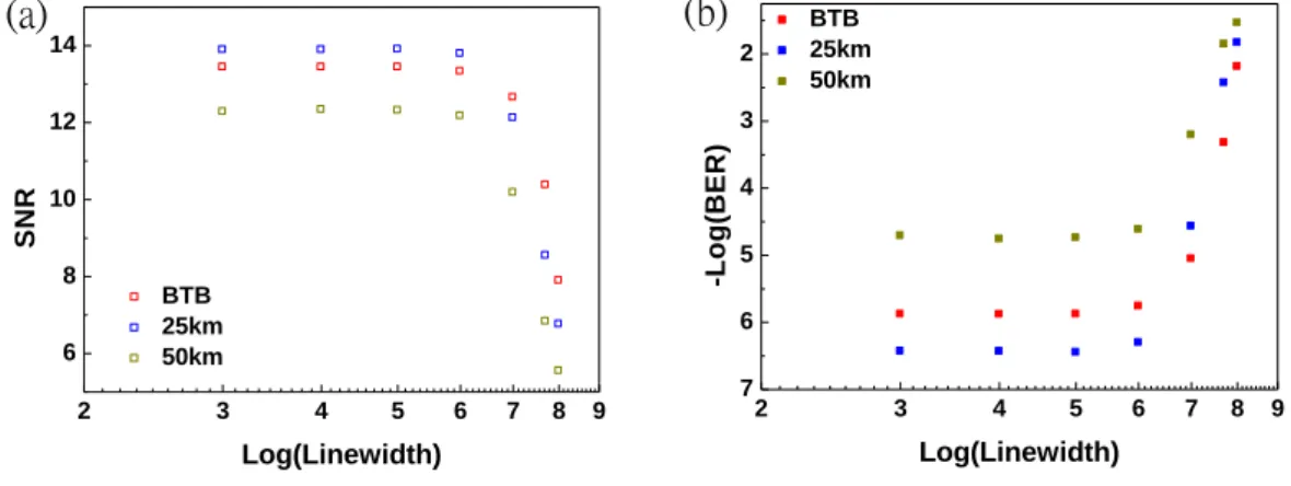
Figure 3-1 the SNR and BER curves of 3.125G bandwidth at 60-GHz millimeter-wave band ... 16
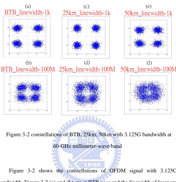
Figure 3-2 constellations of BTB, 25km, 50km with 3.125G bandwidth at 60-GHz millimeter-wave band ... 17
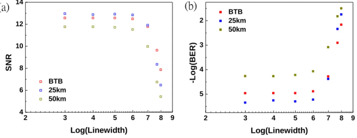
Figure 3-3 the SNR and BER curves of 5G bandwidth at 60-GHz millimeter-wave band ... 18
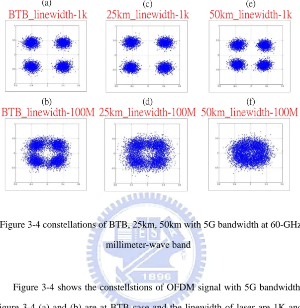
Figure 3-4 constellations of BTB, 25km, 50km with 5G bandwidth at 60-GHz millimeter-wave band ... 19
Figure 3-5 the SNR and BER curves of 7G bandwidth at 60-GHz millimeter-wave band ... 20
Figure 3-6 constellations of BTB, 25km, 50km with 7G bandwidth at 60-GHz millimeter-wave band ... 21
Figure 3-7 the SNR and BER curves of 7G bandwidth at 40-GHz millimeter-wave band ... 22
xi
Figure 3-8 constellations of BTB, 25km, 50km with 7G bandwidth at
40-GHz millimeter-wave band ... 23 Figure 3-9 the SNR and BER curves of 7G bandwidth at 20-GHz
millimeter-wave band ... 24 Figure 3-10 constellations of BTB, 25km, 50km with 7G bandwidth at 20-GHz millimeter-wave band ... 25 Figure 4-1 shows the experimental setup of the proposed system ... 28 Figure 4-2 OPR curve, optical spectrums and constellations of optimal condition with single carrier QPSK ... 30 Figure 4-3 BER curves of single carrier QPSK ... 32 Figure 4-4 optical spectrums and constellations of single carrier QPSK .. 33 Figure 4-5 electrical spectrums of single carrier QPSK ... 34 Figure 4-6 OPR curve, optical spectrums and constellations of optimal condition with single carrier 8QAM ... 35 Figure 4-7 EVM curves of single carrier 8QAM ... 37 Figure 4-8 optical spectrums and constellations of single carrier 8QAM . 38 Figure 4-9 electricdal spectrums of single carrier 8QAM ... 39 Figure 4-10 BB BER curves and eye diagrams of uplink with OOK using single carrier QPSK as downlink signal ... 40 Figure 4-11 optical spectrums of uplink with OOK using single carrier QPSK as downlink signal ... 41 Figure 4-12 the BB BER curves and eye diagrams of uplink with OOK using single carrier 8QAM as downlink signal ... 42 Figure 4-13 optical spectrums of uplink with OOK using single carrier 8QAM as downlink signal ... 43 Figure 5-1 shows OPR curve and optical spectrum for OFDM QPSK ... 44 Figure 5-2 the BER curves and constellations for OFDM QPSK ... 46
xii
Figure 5-3 shows the electrical spectrum for OFDM QPSK ... 47 Figure 5-4 shows OPR curves and optical spectrums of OFDM QPSK at different MI ... 48 Figure 5-5 the BER curves for OFDM QPSK for BTB case at different MI ... 50 Figure 5-6 shows OPR curve and optical spectrum of OFDM QPSK for DFB laser ... 52 Figure 5-7 the BER curves for OFDM QPSK using DFB laser ... 54 Figure 5-8 the BB BER curves and eye diagrams of uplink with OOK using OFDM QPSK as downlink signal ... 56 Figure 5-9 optical spectrums of uplink with OOK using OFDM QPSK as downlink signal ... 57 Figure 5-10 electrical spectrums of uplink with OOK using OFDM QPSK as downlink signal ... 58 Figure 5-11 the BB BER curves and eye diagrams of uplink with OOK using OFDM QPSK as downlink signal ... 59 Figure 5-12 optical spectrums of uplink with OOK using OFDM QPSK as downlink signal ... 60 Figure 5-13 shows BB electrical spectrums. Figure 5-13 (a) is the case of 25km downlink transmission length, and 0km uplink transmission length. Figure 5-13 (b) is the case of 50km downlink transmission length, and 0km uplink transmission length. ... 61
LIST OF TABLES
1
Chapter 1
Introduction
1.1 Why 60-GHz band attracts a great deal of interest
2
Recently, millimeter-wave radio has attracted a great deal of interest from academia, industry, and global standardization bodies due to a number of attractive features of millimeter wave to providemulti-gigabit transmission rate. This enables many new applications such as high definition multimedia interface (HDMI) cable replacement for uncompressed video or audio streaming and multi-gigabit file transferring, all of which intended to provide better quality and user experience.
60-GHz wireless communication system has become a potential candidate for future broadband wireless access network system because the demand of broadband wireless access (BWA) to provide IPTV, HDTV, or Wireless HD application increases, extending the center frequency into millimeter-wave band can achieve higher data rate. It enables up to gigabit-scale connection speeds to be used in indoor WLAN networks or fixed wireless connections in metropolitan areas. The more speed we need the more bandwidth we need. Transmission of several hundred megabits (or even a gigabit) per second requires very large bandwidth, which is available in the millimeter wave area. Modern multimedia applications demand higher data rates, and the trend towards wireless is evident, not only in telephony but also in home and office networking and customer electronics. Many standards have been proposed at 60-GHz band such as IEEE 802.15 WPAN (wireless personal area network), IEEE 802.16 WiMAX, and wireless high definition video services
(WirelessHDTM) [1]. But the 60-GHz wireless millimeter-wave signal has very
high atmospheric loss, and the coverage is limited to a relatively short range. Thanks to the unlimited bandwidth and low transmission loss of optical fiber, 60-GHz RoF technology is a promising solution to provide broadband service
3
[2-4], wide converge, and mobility. But 60-GHz millimeter-wave generation is a serious challenge and arouses considerable interest. Many work have been demonstrated to transmit high data rate signals at 60-GHz millimeter-wave band [2-4, 5].
1.2 Motivation
Thanks to the unlimited bandwidth and low transmission loss of optical fiber, 60-GHz RoF technology is a promising solution to provide wireless broadband communication services, wide converge, and mobility. OFDM modulation format provides a solution with great potential at 60-GHz band [6]. High capacity transmission beyond 10 Gb/s at 60-GHz band within the 7-GHz free licensed band can be achieved due to the high spectrum efficiency of the OFDM modulation format. The uneven channel response can be readily compensated using one-tap equalizer due to the small bandwidth multi-carrier property of the OFDM signal. In summarization, no dispersion induced fading is observed, high spectral efficiency vector signal can be utilized and wavelength reuse is also achieved.
4
Chapter 2
The Concept of New Optical Modulation System
2.1 PrefaceOptical communication systems include three parts: optical transmitter, communication channel and optical receiver. Optical transmitter plays an role to convert an electrical input signal into the corresponding optical signal and then launches it into the optical fiber providing as a communication channel. The utility of an optical receiver is to convert the optical signal back into electrical signal and recover the data transmitted through the lightwave system. In this chapter, we will introduce the external Mach-Zehnder Modulator (MZM), constructing a model of new ROF system.
2.2 Mach-Zehnder Modulator (MZM)
The modulation method of optical signal generation are direct modulation and external modulation. Comparing with the two modulations, if the bit rate of direct modulation signal is above 10-Gb/s, the frequency chirp imposed on signal becomes large enough. Because of this reason, it is difficult to utilize direct modulation to generate microwave/mm-wave. Nevertheless, the band width of signal generated from external modulation can be above 10-Gb/s. In recent year, most RoF systems use external modulation with MZM and Electro-Absorption Modulator (EAM) [7]. Most of the MZMs are based on
LiNbO3 (lithium niobate) technology. The types of LiNbO3 device with the
applied electric field are x-cut and z-cut. With the number of electrode, there
are two types of LiNbO3 device: dual-drive Mach-Zehnder Modulator and
5
2.3 Single-drive Mach-Zehnder modulator
There are two arms and an electrode in the single-drive Mach-Zehnder Modulator. By changing the voltage applied on the electrode, the optical phase in each arm can be controlled. We call that the modulator is in “on” state if the lightwave are in phase. On the other hand, if the lightwave are in opposite phase, the modulator is in “off” state. The lightwave can not propagate by waveguide for output when the modulator is in “off” state.
6
2.4 The architecture of ROF system
2.4.1 Optical transmitter
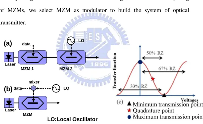
In the optical transmitter system, there are optical source, modulator, local oscillator, etc. So far, most of the RoF system use laser as the optical source. There are a lot of advantages of using laser as optical source. For example, the advantages include compact size, high efficiency, good reliability small emissive area compatible with fiber core dimensions, and possibility of direct modulation at relatively high frequency. Electrical signal converts into optical form by using modulator. Due to the external integrated modulator composing of MZMs, we select MZM as modulator to build the system of optical transmitter. Laser data MZM 1 MZM 2 LO
(a)
Laser data MZM(b)
LO mixer LO:Local OscillatorFigure 2-1 (a) and (b) are two schemes of transmitter and (c) is duty cycle of subcarrier biased at different points in the transfer function. (LO: local
7
Figure 2-1 shows two schemes of optical transmitter and duty cycle of subcarrier biased at different points in the transfer function. In figure 2-1 (a), it is one of the two schemes that we mentioned. In the scheme, it includes one laser, two modulators, one local oscillator, and some data. First MZM is utilized to generate optical carrier which carried the data, and the output optical signal is baseband (BB) signal. The second MZM generates the optical subcarrier which carried the BB signal and then output the RF signal. In figure 2-1 (b), it is another kind of the two schemes of optical transmitter. In the scheme, there are one laser, one modulator,one electrical mixer one local oscillator, and some data. The scheme is used a electrical mixer and a local oscillator (LO) to up-convert elecrical signal and then sent it into a MZM to generate the optical signal. Figure 2-1 (c) depicts the duty cycle of subcarrier biased at different points in the transfer function.
8
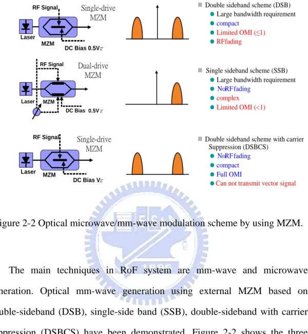
2.4.2 Optical signal generations based on LiNbO3 MZM
Laser RF Signal DC Bias 0.5Vπ MZM Laser RF Signal DC Bias Vπ MZM Laser RF Signal Single-drive MZM Single-drive MZM Dual-drive MZM DC Bias 0.5Vπ MZM
Double sideband scheme (DSB)
Large bandwidth requirement
compact
Limited OMI (≤1)
RFfading
Single sideband scheme (SSB)
Large bandwidth requirement
No RF fading
complex
Limited OMI (<1)
Double sideband scheme with carrier Suppression (DSBCS)
No RF fading
compact
Full OMI
Can not transmit vector signal
Figure 2-2 Optical microwave/mm-wave modulation scheme by using MZM.
The main techniques in RoF system are mm-wave and microwave generation. Optical mm-wave generation using external MZM based on double-sideband (DSB), single-side band (SSB), double-sideband with carrier suppression (DSBCS) have been demonstrated. Figure 2-2 shows the three schemes that we mentioned. For DSB, the optical signal is generated when the DC bias voltage of single-drive MZM is setted at quadrature point. The DSB modulation scheme suffers performance fading problems due to fiber dispersion, resulting in degradation of the receiver sensitivity. So the signals only can be transmitted over several kilo-meters. The RF fading means that when an optical signal is modulated by an electrical RF signal, fiber chromatic dispersion causes the detected RF signal power to have a periodic fading
9
characteristic. Due the reason, the SSB modulation scheme is proposed to overcome the fading issue.
In the SSB modulation scheme, the DC bias voltage of dual-drive MZM is setted at quadrature point and the phase difference of π/2 is applied between the two RF electrodes of the dual-drive MZM. Although the SSB modulation scheme can reduce the fiber dispersion but it suffers worse receiver sensitivity due to the limited optical modulation index (OMI).
In recent year, DSBCS has been demonstrated for optical mm-wave generation. In DSBCS modulation scheme, the DC bias voltage of single-drive MZM is setted at null point. There is no fiber dispersion problem in the scheme It has best receiver sensitivity following transmission over a long distance because the OMI is equal to one. The bandwidth requirment of DSBCS modulation scheme for RF signal, electrical components, electrical amplifier, and optical modulator is lower than DSB and SSB modulation scheme. The sprectral occupancy of DSBCS modulation scheme is the lowest in the three modulation scheme. However, the disadvantage of the DSBCS modulation scheme is that it can not transmit vector signal, such as phase shift keying
(PSK), quadrature amplitude modulation (QAM), or orthogonal
frequency-division multiplexing (OFDM) signals. It only can support on-off keying (OOK) format, which are of utmost importance for wireless application.
10
2.4.3 Communication channel
Figure 2-3 shows the common model of communication channel. Communication channel includes fiber, optical amplifier, etc. Most RoF systems use single mode fiber (SMF) or dispersion compensated fiber (DCF) as the transmission medium. The dispersion will be happened when the optical signal transmits in the fiber. DCF is ulitized to compensate the dispersion phenomenon. The transmission distance of any fiber-optic communication sysem is limited by fiber losses. For long-haul transmission systems, the loss limitation has traditionally been overcome using regenerator witch the optical signal is first converted into an electric current and then regenerated using a transmitter. It is quite expensive and complex for WDM lightwave systems. A method of loss management is utilizing optical amplifier to amplify the optical signal directly without requiring its conversion to electric domain [9]. Most RoF systems use erbium-doped fiber amplifier (EDFA) to amplify the optical signal. The optical bandpss filter (OBPF) is necessary to filter out the ASE noise.
EDFA OBPF
Fiber
Modulated
Optical
Signal
·
EDFA:Erbium-doped Fiber Amplifier
·
OBPF:Optical Bandpass Filter
11
2.4.4 Demodulation of optical millimeter-wave signal
·
PD:Photo-detector
·
LPF:Low-pass Filter
·
BERT:Bit-error-rate Tester
LPF
BERT
LO
PD
mixer
After
transmitting
optical signal
Figure 2-3 The model of receiver in a RoF system.
Figure 2-4 shows the receiver model of the RoF system. As the figure depicts, there are PD, mixer, LO, LPF and BERT. PD usually includes trans-impedance amplifier (TIA) and photo diode. The PIN diode is usually utilized due to it’s lower transit time in the microwave or mm-wave system. TIA function converts photo-current to output voltage.
After PD square-law detection, the BB and RF signals are the same. The RF signal is down converted to baseband signal by using an electrical mixer, and then filtered by low-pass filter (LPF).
The down-converted signal will be sent into a signal analyzer to test its performance, just like bit-error-rate (BER) tester or real time scope, as shown in figure 2-4.
12
LD
PC
data
MZM
LO
mixer
EDFA
OBPF
Fiber
PD
mixer
LPF
BERT
LO
· LD:Laser Diode · PC:Polarization Controller· EDFA:Erbium-doped Fiber Amplifier
· OBPF:Optical Bandpass Filter
· PD:Photodetector
· LPF:Low-pass Filter
· BERT:Bit-error-rate Tester
Figure 2-4 The model of RoF system.
Figure 2-5 shows the model of RoF system. In the model, it concludes transmitter communication channel and receiver. The transmitter combining with communication channel and receiver is called the model of RoF system.
13
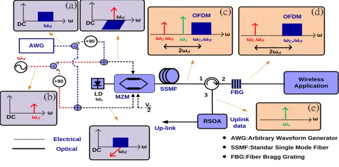
2.5 The new proposed model of optical modulation system
Figure 2-6 depicts the conceptual diagram of the proposed sysem. A dual-drive MZM is biased at quadrrature point to achieve SSB modulation scheme. The OFDM signal is generated from an AWG and the OFDM optical sideband is shown in figure 2-6 (a). A new optical carrier is generated from a
pure sinusoidal signal with frequency of ωrf. In the figure 2-6 (b), the optical
sideband of sinusoidal is located at frequency ωrf. In order to achieve tandem
SSB modulation scheme, a 900 phase shifter is added to the upper path of
OFDM signal and the lower path of the sinusoidal signal. The upper path of OFDM signal and sinusoidal signal are combined and sent into one of the electrode of the dual-drive MZM. On the other hand, the lower path of OFDM signal and sinusoidal signal are also combined and sent into the other electrode of the dual-drive MZM.
At the output of the dual-drive MZM, the optical spectrum is shown in
figure 2-6 (C). There are original optical carrier (ωc), new optical carrier
(ωc − ωrf), and OFDM optical sideband (ωc + ωrf) in the optical spectrum.
And then, after SSMF transmission, a fiber bragg grating (FBG) and optical circulator are utilized to separate the original optical carrier for the reuse of
uplink data. After the FBG, the OFDM optical sideband (ωc+ ωrf) and the new
optical carrier (ωc − ωrf) are received for wireless application. The figure 2-6
(d) shows the optical spectrum which includes the OFDM optical sideband
(ωc + ωrf) and the new optical carrier (ωc − ωrf), and the original optical
carrier is separated by FBG. The original optical carrier using a RSOA [10] for uplink application. The figure 2-6 (e) shows the separated original optical carrier. In this work, generation and transmission of 60-GHz signal using
14
modified tandem single sideband (TSSB) modulation scheme [11].
LD Electrical Optical +90∘ AWG Vπ 2 SSMF 1 2 3 FBG Wireless Application MZM RSOA ωrf ωrf DC DC ω ω ωc ωrf ωrf DC ω Up-link ω ωc Uplink data OFDM ωC+ωrf ωC-ωrf 2ωrf ω OFDM ωC+ωrf ωC-ωrf ωc 2ωrf ω ωrf DC ω +90∘
· AWG:Arbitrary Waveform Generator
· SSMF:Standar Single Mode Fiber
· FBG:Fiber Bragg Grating
(a)
(b)
(c) (d)
(e)
Figure 2-5 Concept of the proposed system. (LD: laser diode, MZM: Mach-Zehnder modulator, SSMF:standar single mode fiber, FBG: fiber bragg
15
Chapter 3
The Theoretical Simulations of Proposed System
3.1 prefaceSome theoretical simulations are shown in this chapter. The VPI software is utilized here. The system is modified TSSB as shown in figure 2-6. In the simulation, the signal is OFDM signal, and the issue that we discuss is the linewidth of the laser source. First part, the bandwidth of the OFDM signals are 3.125G, 5G, 7G, respectively and the signals are all located at 60-GHz millimeter-wave band. Second part, the bandwidth of the OFDM signal is all 7G, but the signals are located at 60-GHz, 40-GHz, 20-GHz millimeter-wave band, respectively. In next several sections, the diagrams of signal to noise ratio (SNR) and BER versus linewidth of the laser.
In the theorical simulation, the input power of photodetector is setted at -8.5 dBm. There are three cases about BTB, 25km transmission length, 50km transmission length in the simulations which are tested. The range of laser linewidth which we discuss is from 1K to 100000K. In the range of laser
linewidth, the division which we set is per 101. We will itemize to illustrate
16
3.2 Theoretical simulation of proposed system for OFDM signal with 3.125G bandwidth at 60-GHz millimeter-wave band
2 3 4 5 6 7 8 9 8 7 6 5 4 3 2 1 BTB 25km 50km BTB 25km 50km -L o g (B E R ) Log(Linewidth) (a) (b) 2 3 4 5 6 7 8 9 6 8 10 12 14 16 BTB 25km 50km S N R Log(Linewidth)
Figure 3-1 the SNR and BER curves of 3.125G bandwidth at 60-GHz millimeter-wave band
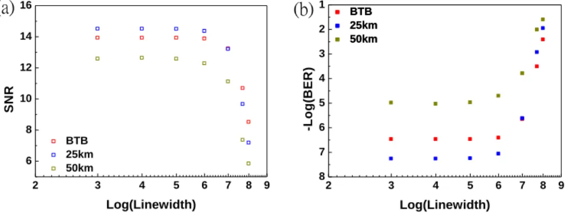
In the section, the OFDM signal with 3.125G bandwidth is utilized as the signal source. The system is modified TSSB scheme. In the simulation, the BTB, 25km transmission, 50km transmission cases are tested. The saved files are analyzed using outline MATLAB program. Figure 3-1 (a) shows the diagram of signal to noise ratio (SNR) versus linewidth of laser source. In the figure, when the linewidth of laser increases, the SNR gets worse at BTB, 25km transmission length, 50km transmission length cases. Figure 3-1 (b) shows the diagram of BER versus linewidth of laser source. When the linewidth of laser increases, the BER gets worse at BTB, 25km transmission length, 50km transmission length cases. Compared with the figure3-1 (a) and (b), if the SNR is much better, the BER is also much better at the three cases. In figure 3-1, we find that the SNR and BER at 25km transmission case is better than at BTB case due to the self modulation of the fiber.
17
BTB_linewidth-1k
BTB_linewidth-100M
25km_linewidth-1k
50km_linewidth-1k
25km_linewidth-100M 50km_linewidth-100M
(a) (b) (c) (d) (e) (f)Figure 3-2 constellations of BTB, 25km, 50km with 3.125G bandwidth at 60-GHz millimeter-wave band
Figure 3-2 shows the constellstions of OFDM signal with 3.125G bandwidth. Figure 3-2 (a) and (b) are at BTB case and the linewidth of laser are 1K and 100M respectively. Figure 3-2 (c) and (d) are at 25km transmission case and figure 3-2 (e) and (f) are at 50km transmission case. In figure 3-2 (c) and (e), the linewidth of laser source is 1K at 25km transmission and 50km transmission case respectively. As shown in figure 3-2 (d) and (f), the linewidth of laser source is 100M at 25km transmission and 50km transmission case respectively. When the linewidth of laser source is 1K, the constellation is very clear. The constellation gets blured when the linewidth of laser source increases at the three cases (BTB, 25km, 50km).
18
3.3 Theoretical simulation of proposed system for OFDM signal with 5G bandwidth at 60-GHz millimeter-wave band
2 3 4 5 6 7 8 9 7 6 5 4 3 2 BTB 25km 50km -L o g (B E R ) Log(Linewidth) (a) (b) 2 3 4 5 6 7 8 9 6 8 10 12 14 BTB 25km 50km S N R Log(Linewidth)
Figure 3-3 the SNR and BER curves of 5G bandwidth at 60-GHz millimeter-wave band
In the section, the OFDM signal with 5G bandwidth is utilized as the signal source. The system is modified TSSB scheme. In the simulation, the BTB, 25km transmission, 50km transmission cases are tested. The saved files are analyzed using outline MATLAB program. Figure 3-3 (a) shows the diagram of SNR versus linewidth of laser source. In the figure, when the linewidth of laser increases, the SNR gets worse at BTB, 25km transmission length, 50km transmission length cases. Figure 3-3 (b) shows the diagram of BER versus linewidth of laser source. When the linewidth of laser increases, the BER gets worse at BTB, 25km transmission length, 50km transmission length cases. Compared with the figure3-3 (a) and (b), if the SNR is much better, the BER is also much better at the three cases. In figure 3-3, we find that the SNR and BER at 25km transmission case is better than at BTB case because the self modulation of the fiber.
19
BTB_linewidth-1k
BTB_linewidth-100M
25km_linewidth-1k
50km_linewidth-1k
25km_linewidth-100M 50km_linewidth-100M
(a) (b) (d) (c) (e) (f)Figure 3-4 constellations of BTB, 25km, 50km with 5G bandwidth at 60-GHz millimeter-wave band
Figure 3-4 shows the constellstions of OFDM signal with 5G bandwidth. Figure 3-4 (a) and (b) are at BTB case and the linewidth of laser are 1K and 100M respectively. Figure 3-4 (c) and (d) are at 25km transmission case and figure 3-4 (e) and (f) are at 50km transmission case. In figure 3-4 (c) and (e), the linewidth of laser source is 1K at 25km transmission and 50km transmission case respectively. As shown in figure 3-4 (d) and (f), the linewidth of laser source is 100M at 25km transmission and 50km transmission case respectively. When the linewidth of laser source is 1K, the constellation is very clear. The constellation gets blured when the linewidth of laser source increases at the three cases (BTB, 25km, 50km).
20
3.4 Theoretical simulation of proposed system for OFDM signal with 7G bandwidth at 60-GHz millimeter-wave band
2 3 4 5 6 7 8 9 5 4 3 2 BTB 25km 50km -L o g (B E R ) Log(Linewidth) (a) (b) 2 3 4 5 6 7 8 9 4 6 8 10 12 14 BTB 25km 50km S N R Log(Linewidth)
Figure 3-5 the SNR and BER curves of 7G bandwidth at 60-GHz millimeter-wave band
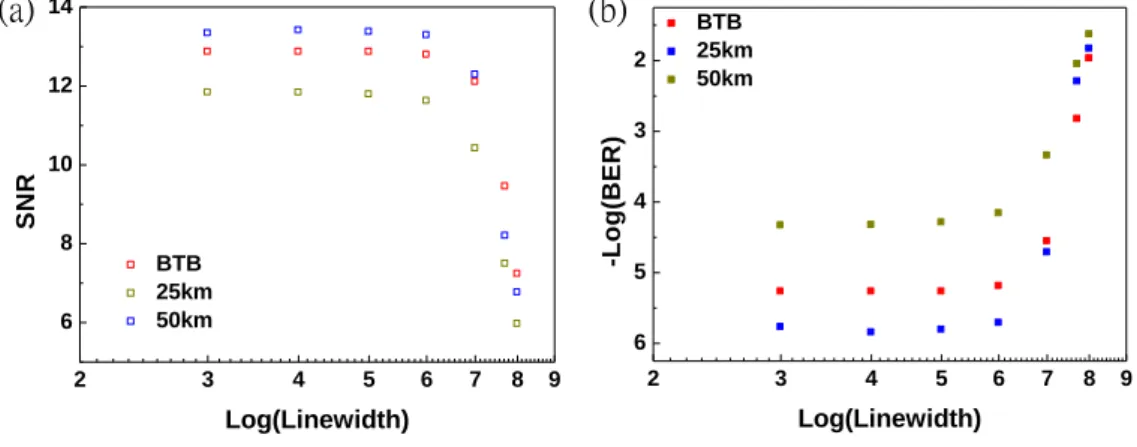
In the section, the OFDM signal with 7G bandwidth is utilized as the signal source. The system is modified TSSB scheme. In the simulation, the BTB, 25km transmission, 50km transmission cases are tested. The saved files are analyzed using outline MATLAB program. Figure 3-5 (a) shows the diagram of SNR versus linewidth of laser source. In the figure, when the linewidth of laser increases, the SNR gets worse at BTB, 25km transmission length, 50km transmission length cases. Figure 3-5 (b) shows the diagram of BER versus linewidth of laser source. When the linewidth of laser increases, the BER gets worse at BTB, 25km transmission length, 50km transmission length cases. Compared with the figure3-5 (a) and (b), if the SNR is much better, the BER is also much better at the three cases. In figure 3-5, we find that the SNR and BER at 25km transmission case is better than at BTB case because the self modulation of the fiber.
21
BTB_linewidth-1k
BTB_linewidth-100M
25km_linewidth-1k
50km_linewidth-1k
25km_linewidth-100M 50km_linewidth-100M
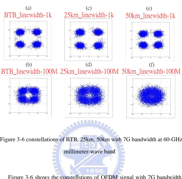
(a) (b) (c) (d) (e) (f)Figure 3-6 constellations of BTB, 25km, 50km with 7G bandwidth at 60-GHz millimeter-wave band
Figure 3-6 shows the constellstions of OFDM signal with 7G bandwidth. Figure 3-6 (a) and (b) are at BTB case and the linewidth of laser are 1K and 100M respectively. Figure 3-6 (c) and (d) are at 25km transmission case and figure 3-6 (e) and (f) are at 50km transmission case. In figure 3-6 (c) and (e), the linewidth of laser source is 1K at 25km transmission and 50km transmission case respectively. As shown in figure 3-6 (d) and (f), the linewidth of laser source is 100M at 25km transmission and 50km transmission case respectively. When the linewidth of laser source is 1K, the constellation is very clear. The constellation gets blured when the linewidth of laser source increases at the three cases (BTB, 25km, 50km).
22
3.5 Theoretical simulation of proposed system for OFDM signal with 7G bandwidth at 40-GHz millimeter-wave band
2 3 4 5 6 7 8 9 6 5 4 3 2 BTB 25km 50km -L o g (B E R ) Log(Linewidth) (a) (b) 2 3 4 5 6 7 8 9 6 8 10 12 14 BTB 25km 50km S N R Log(Linewidth)
Figure 3-7 the SNR and BER curves of 7G bandwidth at 40-GHz millimeter-wave band
In the section, the OFDM signal with 7G bandwidth is utilized as the signal source. The system is modified TSSB scheme. In the simulation, the BTB, 25km transmission, 50km transmission cases are tested. The saved files are analyzed using outline MATLAB program. Figure 3-7 (a) shows the diagram of SNR versus linewidth of laser source. In the figure, when the linewidth of laser increases, the SNR gets worse at BTB, 25km transmission length, 50km transmission length cases. Figure 3-7 (b) shows the diagram of BER versus linewidth of laser source. When the linewidth of laser increases, the BER gets worse at BTB, 25km transmission length, 50km transmission length cases. Compared with the figure3-7 (a) and (b), if the SNR is much better, the BER is also much better at the three cases. In figure 3-7, we find that the SNR and BER at 25km transmission case is better than at BTB case because the self modulation of the fiber.
23
BTB_linewidth-1k
BTB_linewidth-100M
25km_linewidth-1k
50km_linewidth-1k
25km_linewidth-100M 50km_linewidth-100M
(a) (b) (c) (d) (e) (f)Figure 3-8 constellations of BTB, 25km, 50km with 7G bandwidth at 40-GHz millimeter-wave band
Figure 3-8 shows the constellstions of OFDM signal with 7G bandwidth. Figure 3-8 (a) and (b) are at BTB case and the linewidth of laser are 1K and 100M respectively. Figure 3-8 (c) and (d) are at 25km transmission case and figure 3-8 (e) and (f) are at 50km transmission case. In figure 3-8 (c) and (e), the linewidth of laser source is 1K at 25km transmission and 50km transmission case respectively. As shown in figure 3-8 (d) and (f), the linewidth of laser source is 100M at 25km transmission and 50km transmission case respectively. When the linewidth of laser source is 1K, the constellation is very clear. The constellation gets blured when the linewidth of laser source increases at the three cases (BTB, 25km, 50km).
24
3.6 Theoretical simulation of proposed system for OFDM signal with 7G bandwidth at 20-GHz millimeter-wave band
2 3 4 5 6 7 8 9 6 5 4 3 2 BTB 25km 50km -L o g (B E R ) Log(Linewidth) (a) (b) 2 3 4 5 6 7 8 9 6 8 10 12 14 BTB 25km 50km S N R Log(Linewidth)
Figure 3-9 the SNR and BER curves of 7G bandwidth at 20-GHz millimeter-wave band
In the section, the OFDM signal with 7G bandwidth is utilized as the signal source. The system is modified TSSB scheme. In the simulation, the BTB, 25km transmission, 50km transmission cases are tested. The saved files are analyzed using outline MATLAB program. Figure 3-9 (a) shows the diagram of SNR versus linewidth of laser source. In the figure, when the linewidth of laser increases, the SNR gets worse at BTB, 25km transmission length, 50km transmission length cases. Figure 3-9 (b) shows the diagram of BER versus linewidth of laser source. When the linewidth of laser increases, the BER gets worse at BTB, 25km transmission length, 50km transmission length cases. Compared with the figure3-9 (a) and (b), if the SNR is much better, the BER is also much better at the three cases. In figure 3-9, we find that the SNR and BER at 25km transmission case is better than at BTB case because the self modulation of the fiber.
25
BTB_linewidth-1k
BTB_linewidth-100M
25km_linewidth-1k
50km_linewidth-1k
25km_linewidth-100M 50km_linewidth-100M
(a) (b) (c) (d) (e) (f)Figure 3-10 constellations of BTB, 25km, 50km with 7G bandwidth at 20-GHz millimeter-wave band
Figure 3-10 shows the constellstions of OFDM signal with 7G bandwidth. Figure 3-10 (a) and (b) are at BTB case and the linewidth of laser are 1K and 100M respectively. Figure 3-10 (c) and (d) are at 25km transmission case and figure 3-10 (e) and (f) are at 50km transmission case. In figure 3-10 (c) and (e), the linewidth of laser source is 1K at 25km transmission and 50km transmission case respectively. As shown in figure 3-10 (d) and (f), the linewidth of laser source is 100M at 25km transmission and 50km transmission case respectively. When the linewidth of laser source is 1K, the constellation is very clear. The constellation gets blured when the linewidth of laser source increases at the three cases (BTB, 25km, 50km).
26
3.7 Simulation comparison
First, in 3.2, 3.3, 3.4 prat, the OFDM signals are also located at 60-GHz millimeter-wave band but the bandwidth of the OFDM signals are 3.125G, 5G and 7G respectively. Compared with the three parts, the difference between the three parts is bandwidth of OFDM signal. From the three parts, when the bandwidth of OFDM signal increases, the SNR and BER get worse as shown in figure 3-1, 3-3, 3-5 and the constellation gets blured as shown in figure 3-2, 3-4, 3-6.
Second, in 3.4, 3.5, 3.6 part, the bandwidth of OFDM signals are all 7G but the OFDM signals are located at 60-GHz, 40-GHz, 20-GHz millimeter-wave band respectively. Compared with the three parts, the difference between the three parts is millimeter-wave band which is the OFDM signal located. The SNR and BER is almost the same as shown in figure 3-5, 3-7, 3-9 and the constellations are clear as shown in figure 3-6, 3-8, 3-10.
27
Chapter 4
Experimental Results of Proposed System for Single Carrier
4.1 prefaceIn chapter 3, we provide the simulation for the concept of the proposed system. Therefore, the result can be tried to apply to the radio-over-fiber system. In the chapter, we will build the experimental setup for the proposed system. In the proposed system, we use tunable laser and distributed feedback (DFB) laser to fit the linewidth of the laser source because the linewidth of tunable laser and DFB laser are located at the range of several KHz and several MHz respectively.
28
4.2 Experimental results of TSSB
4.2.1 Experiment setup
Figure 4-1 displays the experimental setup of proposed system. Tunable lasers and DFB lasers are used to be the optical source. The OFDM signal with 88 carriers is gnerated from an arbitrary waveform generator (AWG). Every subcarrier is encoded with 78.125MHz QPSK symbol. The inverse fast Fourier transform (IFFT) size is 256. Because the sampling rate is 20GHz, so the total bandwidth of OFDM signal is (20GHz/256)*88=6.875GHz (about 7GHz). The OFDM signal is up-converted to 30GHz using an electrical mixer. The OFDM signal is generated on BB, the lower sideband and upper sideband of the up-converted electrical signal are not mutually independent. Because every subcarrier is demodulated independently,the limit between the subcarriers’ symbols has negligible effect on the system performance.
LD Phase shift +90∘ Phase shift +90∘ 30 GHz x AWG Vπ 2 EDFA MZM FBG O/E LPF BERT Electrical Optical 1 2 3 RSOA 1.25 Gb/sec OOK SSMF E/O 60 GHz BPF Scope 55 GHz Wireless Remote Node SSMF · LD:Laser Diode
· AWG:Arbitrary Waveform Generator · EDFA:Erbium-doped Fiber Amplifier · SSMF:Standar Single Mode Fiber · FBG:Fiber Bragg Grating
· PD:Photodetector · BPF:Bandpass Filter
· RSOA:Reflective Semiconductor Optical Amplifier · LPF:Low-pass Filter
· BERT:Bit-error-rate Tester
Figure 4-1 shows the experimental setup of the proposed system
29
bandwidth of the signal is about 7-GHz, and the data rate is about 14-Gb/sec. With a
900 hybrid coupler, the 30-GHz RF OFDM signal is split two paths. A 30-GHz
sinusoidal signal is also split two paths using 900 hybrid coupler. As Figure 4-1
shows, the upper 30-GHz RF OFDM signal combines with the upper 30-GHz sinusoidal signal and the lower 30-GHz RF OFDM signal combines with the lower 30-GHz sinusoidal signal. These combined signals are amplified to drive the dual-drive MZM. The MZM is biased at quadrature point to achieve SSB modulation scheme. At the output of the MZM, an EDFA is employed to boost the total optical power. After the EDFA, the optical power is transmitted through the SSMF, At the output of the SSMF, the circulator is employed to separate the original optical carrier and the other signals. At 2 port of the circulator, the FBG is utilized to eliminate the optical carrier. At remote node, the 60-GHz RF OFDM signal is obtained from the beating signal of the OFDM optical sideband and new optical carrier at a 60-GHz photo diode. A bandpass filter (BPF) with center frequency 60-GHz is employed to filter out the 60-GHz electrical OFDM signal. The 60-GHz OFDM signal is down-converted to 5-GHz using an electrical mixer with 55-GHz LO signal.
The down-converted 5-GHz OFDM signal is sent to a real time scope to capture the time domain waveform. The OFDM signal is demodulated with off-line digital signal processing (DSP) program. The demodulation process includes synchronization, Fast Fourier Transform (FFT), one-tap equalization, and QPSK symbol decoding. The BER is obtained from the measured error vector magnitude (EVM). At 3 port of the circulator, the original optical carrier is utilized for uplink application with RSOA and the electrical signal 1.25-Gb/s OOK with generating from a pattern generator. After RSOA and SSMF, the uplink signal is received by a low-speed photo diode. After a LPF, the BER of the uplink signal is obtained directly using bit error rate tester (BERT).
30
4.3 Experimental results of TSSB using single carrier QPSK
4.3.1 Optimal condition of single carrier QPSK
-8 -6 -4 -2 0 2 8 7 6 5 4 3 2 QPSK_with FFE QPSK_without FFE -L o g (B E R ) OPR 1554.4 1554.6 1554.8 1555.0 1555.2 1555.4 -55 -50 -45 -40 -35 -30 -25 P o w e r( d B m ) Wavelength(nm) 1554.4 1554.6 1554.8 1555.0 1555.2 1555.4 -55 -50 -45 -40 -35 -30 -25 P o w e r( d B m ) Wavelength(nm) 1554.4 1554.6 1554.8 1555.0 1555.2 1555.4 -55 -50 -45 -40 -35 -30 -25 P o w e r( d B m ) Wavelength(nm) 1554.4 1554.6 1554.8 1555.0 1555.2 1555.4 -55 -50 -45 -40 -35 -30 -25 P o w e r( d B m ) Wavelength(nm) 1554.4 1554.6 1554.8 1555.0 1555.2 1555.4 -55 -50 -45 -40 -35 -30 -25 P o w e r( d B m ) Wavelength(nm) 1554.4 1554.6 1554.8 1555.0 1555.2 1555.4 -55 -50 -45 -40 -35 -30 -25 P o w e r( d B m ) Wavelength(nm) (a) (b) (c) (d) (e) (f)
Figure 4-2 OPR curve, optical spectrums and constellations of optimal condition with single carrier QPSK
In this part , the signal is single carrier QPSK with data rate 2.5Gb/s. The optical power ratio (OPR) is power of clock over QPSK signal. The OPR is a very important factor which effects the receiver sensitivity of signal. Figure 4-2 shows the BER versus OPR curve, optical spectrums and constellations. In optical spectrum, the left sideband is single carrier QPSK signal and the right sidband is clock signal. The original optical carrier is removed by FBG. Figure 4-2 (a) and (b) shows the optical spectrums and constellations when the OPR is -8. In optical spectrum, the left sideband is single carrier QPSK signal and the right sidband is clock signal. The original optical carrier is removed by FBG. In figure 4-2, the BER of blue curve is better than green curve because the
31
feed-forward equalizer (FFE) with 16 taps is utilized here. Figure 4-2 (c) and (d) shows the optical spectrums and constellations when the OPR is 0. And the same, figure 4-2 (e) and (f) shows the optical spectrums and constellations when the OPR is 1. In optical spectrum, the left sideband is single carrier QPSK signal and the right sidband is clock signal. The original optical carrier is removed by FBG. In the figure, the best receiver sensitivity is obtained when the OPR is 0 and the constellation is very clear.
32 4.3.2 Transmission results -16 -15 -14 -13 -12
10
9
8
7
6
5
4
3
2
QPSK_BTB_with FFE QPSK_BTB_w/o FFE QPSK_50km_With FFE QPSK_50km_w/o FFE-L
o
g
(B
E
R
)
Power(dBm)
Figure 4-3 BER curves of single carrier QPSK
Figure 4-3 shows the curve of receiver power versus the BER. The blue curve is back-to-back (BTB) case, and the red curve is transmission length with 50-km SSMF. The full symbol represents the FFE is utilized, and the hollow symbol represents the FFE is not used. In figure 4-3, when the receiver sensitivity is -12 dBm, the order of BER can achieve to -10. The order of
BER is improved from 10−10 to 10−4 with -8 dBm optical power. The
receiver power penalty at BER of 10−10 with FFE (10−4 without FFE) is less
33 1 5 5 4 .4 1 5 5 4 .6 1 5 5 4 .8 1 5 5 5 .0 1 5 5 5 .2 1 5 5 5 .4 - 5 5 - 5 0 - 4 5 - 4 0 - 3 5 - 3 0 - 2 5 P o w e r (d B m ) W a v e le n g t h ( n m )
BTB
With FFE
Without FFE
50km
With FFE
Without FFE
1 5 5 4 .6 1 5 5 4 .8 1 5 5 5 .0 1 5 5 5 .2 1 5 5 5 .4 - 7 0 - 6 5 - 6 0 - 5 5 - 5 0 - 4 5 - 4 0 - 3 5 - 3 0 - 2 5 P o w e r (d B m ) W a v e le n g t h ( n m )
(a)
(b)
Figure 4-4 optical spectrums and constellations of single carrier QPSK
Figure 4-4 shows optical spectrums and constellations with receiver power -12 dBm. For (a), it is BTB case. The left is optical spectrums, and the middle and the right are constellations. In optical spectrums, the left sideband is QPSK signal, the right sideband is clock signal, the original optical carrier is removed by FBG. The middle constellations is with FFE compensated the uneven frequency responses. The right constellations is without FFE. For (b), it is 50-km SSMF transmission case. The 50-km SSMF transmission case is similar to the BTB case. The left is optical spectrums, and the middle and the right are constellations. In optical spectrums, the left sideband is single carrier QPSK signal, the right sideband is clock signal, the original optical carrier is removed by FBG. The middle constellations is with FFE, and The right constellations is
34 without FFE. 1 2 3 4 -90 -80 -70 -60 -50 -40 -30 -20 -10 0 P o w e r( d B m ) Frequency(GHz)
After AWG Upconvert to 30G
27 28 29 30 31 32 33 -120 -110 -100 -90 -80 -70 -60 -50 -40 -30 P o w e r( d B m ) Frequency(GHz) Downconvert to 2.5G 1 2 3 4 -110 -100 -90 -80 -70 -60 -50 -40 -30 -20 -10 0 P o w e r( d B m ) Frequency(GHz) (a) (b) (c)
Figure 4-5 electrical spectrums of single carrier QPSK
Figure 4-5 shows electricdal spectrums. (a) is the electrical spectrum after an AWG. (b) is the QPSK signal up-converted to 30-GHz with a electrical mixer. (c) is the RF QPSK signal down-converted to 2.5-GHz with a electrical mixer.
35
4.4 Experimental results of TSSB using single carrier 8QAM
4.4.1 Optimal condition of single carrier 8QAM
-6 -4 -2 0 2 4 6 15 20 25 30 35 40 8QAM_With FFE 8QAM_Without FFE E V M (% ) OPR 1554.4 1554.6 1554.8 1555.0 1555.2 1555.4 -55 -50 -45 -40 -35 -30 -25 -20 P o w e r( d B m ) Wavelength(nm) 1554.4 1554.6 1554.8 1555.0 1555.2 1555.4 -55 -50 -45 -40 -35 -30 -25 -20 P o w e r( d B m ) Wavelength(nm) 1554.4 1554.6 1554.8 1555.0 1555.2 1555.4 -55 -50 -45 -40 -35 -30 -25 P o w e r( d B m ) Wavelength(nm) 1554.4 1554.6 1554.8 1555.0 1555.2 1555.4 -55 -50 -45 -40 -35 -30 -25 P o w e r( d B m ) Wavelength(nm) 1554.4 1554.6 1554.8 1555.0 1555.2 1555.4 -55 -50 -45 -40 -35 -30 -25 P o w e r( d B m ) Wavelength(nm) 1554.4 1554.6 1554.8 1555.0 1555.2 1555.4 -55 -50 -45 -40 -35 -30 -25 P o w e r( d B m ) Wavelength(nm) (a) (b) (c) (d) (e) (f)
Figure 4-6 OPR curve, optical spectrums and constellations of optimal condition with single carrier 8QAM
In this part , the signal is single carrier 8QAM with data rate 2.34375Gb/s. The OPR is power of clock over 8QAM signal. The OPR is a very important factor which effects the receiver sensitivity of signal. Figure 4-6 shows the error vector magnitude (EVM) versus OPR curve, optical spectrums and constellations. The EVM is defined as
2 1 2 max 1
[%]
100 [
N r i]
iEVM
d
d
N
d
Where dr and
d
i are the received and ideal symbols respectively, and dmaxis the maximum symbol vector in the constellation. Figure 4-6 (a) and (b) shows the optical spectrums and constellations when the OPR is -6. In figure
36
4-6, the EVM of blue curve is better than green curve because the FFE with 16 taps is utilized here. Figure 4-6 (c) and (d) shows the optical spectrums and constellations when the OPR is -1. In optical spectrum, the left sideband is single carrier 8QAM signal and the right sidband is clock signal. The original optical carrier is removed by FBG. And the same, figure 4-6 (e) and (f) shows the optical spectrums and constellations when the OPR is -5. In optical spectrum, the left sideband is single carrier 8QAM signal and the right sidband is clock signal. The original optical carrier is removed by FBG. In the figure, the best receiver sensitivity is obtained when the OPR is 0 and the constellation is very clear.
37 4.4.2 Transmission results
-20
-18
-16
-14
-12
-10
-8
10
15
20
25
30
35
40
45
BTB with FFE BTB w/o FFE 50km with FFE 50km w/o FFEE
V
M
(%
)
POWER(dBm)
Figure 4-7 EVM curves of single carrier 8QAM
Figure 4-7 illustrates the curve of receiver power versus the EVM. The blue curve is BTB case, and the red curve is transmission length with 50-km. SSMF. The full symbol represents the FFE is utilized, and the hollow symbol represents the FFE is not used. In figure 4-7, Before FFE, there is an EVM fluctuation due to receiver saturation with the increasing of the received optical power. However, the FFE can compensate not only the uneven frequency response but also the receiver saturation. After the FFE, the EVM is improved from 18.9% to 15.7 % with -8 dBm optical power. The power penalty at EVM of 15% with FFE (18% without FFE) is less than 0.2 dB at BTB case and 50-km SSMF transmission case.
38 1554.4 1554.6 1554.8 1555.0 1555.2 1555.4 -55 -50 -45 -40 -35 -30 -25 P o w e r( d B m ) Wavelength(nm) BTB Without FFE With FFE 50km Without FFE With FFE 1554.4 1554.6 1554.8 1555.0 1555.2 1555.4 -70 -65 -60 -55 -50 -45 -40 -35 -30 P o w e r( d B m ) Wavelength(nm)
Figure 4-8 optical spectrums and constellations of single carrier 8QAM
Figure 4-8 shows optical spectrums and constellations with receiver power -8 dBm. For (a), it is BTB case. The left is optical spectrums, the middle and the right are constellations. In optical spectrums, the left sideband is 8QAM signal, the right sideband is clock signal, the original optical carrier is removed by FBG. The middle constellations is with FFE compensated the uneven frequency responses. The right constellations is without FFE. For (b), it is 50-km SSMF transmission case. The 50-km SSMF transmission case is similar to the BTB case. The left is optical spectrums, and the middle and the right are constellations. In optical spectrums, the left sideband is 8QAM signal, the right sideband is clock signal, the original optical carrier is removed by FBG. The middle constellations is with FFE, and The right constellations is without FFE.
39
After AWG Upconvert to 30G Downconvert to 2.5G
1 2 3 4 -80 -70 -60 -50 -40 -30 -20 -10 0 P o w e r( d B m ) Frequency(GHz) 27 28 29 30 31 32 33 -120 -110 -100 -90 -80 -70 -60 -50 -40 -30 P o w e r( d B m ) Frequency(GHz) 1 2 3 4 -120 -110 -100 -90 -80 -70 -60 -50 -40 -30 -20 -10 0 P o w e r( d B m ) Frequency(GHz) (a) (b) (c)
Figure 4-9 electricdal spectrums of single carrier 8QAM
Figure 4-9 shows electricdal spectrums. (a) is the electrical spectrum after an AWG. (b) is the 8QAM signal up-converted to 30-GHz with a electrical mixer. (c) is the RF 8QAM signal down-converted to 2.5-GHz with a electrical mixer.
40
4.5 Experimental results of TSSB for uplink with OOK using single carrier QPSK as downlink signal
4.5.1 Uplink with OOK using single carrier QPSK as downlink signal
Downlink_50km-Uplink_0km (BTB) Downlink_50km-Uplink_50km (50km) PD_Input_-18.5dBm_130mv/div;200ps/div -29 -28 -27 -26 -25 109 8 7 6 5 4 3 2 BTB 50km -L o g (B E R ) Power(dBm) (b) (c) (a)
Figure 4-10 BB BER curves and eye diagrams of uplink with OOK using single carrier QPSK as downlink signal
Figure 4-10 shows BB BER curves and eye diagrams of uplink 1.25-Gb/s OOK signal for downlink single carrier QPSK signal. In (a), the full symbol means BTB case. The hollow symbol means 50-km SSMF case. The order of
BER can achieve to 10−10 when the receiever optical power is -25.2 dBm.
After 50-km SSMF transmission, there is no significant receiver power penalty of the OOK uplink signal. Figure 4-10 (b) is BTB case, and (c) is 50-km SSMF transmission case. These two eye diagrams are very clear. The eye diagrams are catched by digital communications analyzer (DCA) when the input power is -18.5 dBm. The vertical scale of these two eye diagrams is 130mv/div, and the horizontal scale of these two eye diagrams is 200ps/div.
41
Before Circulator After FBG
Original optical carrier without uplink signal
Original optical carrier with uplink signal 1 5 5 4 .4 1 5 5 4 .6 1 5 5 4 .8 1 5 5 5 .0 1 5 5 5 .2 1 5 5 5 .4 - 5 0 - 4 0 - 3 0 P o w e r (d B m ) W a v e le n g t h ( n m ) 1 5 5 4 .4 1 5 5 4 .6 1 5 5 4 .8 1 5 5 5 .0 1 5 5 5 .2 1 5 5 5 .4 - 8 0 - 7 0 - 6 0 - 5 0 - 4 0 - 3 0 - 2 0 - 1 0 0 P o w e r (d B m ) W a v e le n g t h ( n m ) 1 5 5 4 .4 1 5 5 4 .6 1 5 5 4 .8 1 5 5 5 .0 1 5 5 5 .2 1 5 5 5 .4 - 6 0 - 5 0 - 4 0 - 3 0 - 2 0 - 1 0 0 P o w e r (d B m ) W a v e le n g t h ( n m ) 1 5 5 4 .6 1 5 5 4 .8 1 5 5 5 .0 1 5 5 5 .2 1 5 5 5 .4 - 8 0 - 7 0 - 6 0 - 5 0 - 4 0 - 3 0 - 2 0 P o w e r (d B m ) W a v e le n g t h ( n m ) (a) (b) (c) (d)
Figure 4-11 optical spectrums of uplink with OOK using single carrier QPSK as downlink signal
Figure 4-11 shows optical spectrums. In (a), it is at the output of the MZM case. The left sideband is single carrier QPSK signal, the middle sideband is original optical carrier, and the right sideband is clock signal. In (b), The left sideband is single carrier QPSK signal, and the right sideband is clock signal. The original optical carrier is removed by FBG. In (c), the middle sideband is original optical carrier without 1.25Gb/s OOK signal. The original optical carrier is separated from the other optical sidebands by using circulator and FBG. In (d), it is original optical carrier with 1.25Gb/s OOK signal for uplink application using RSOA.