在BGM 模型下固定交換利率商品之效率避險與評價 - 政大學術集成

全文

(1)國立政治大學金融系博士論文指導教授: 廖四郎博士. 在 BGM 模型下固定交換利率商品之效率避險與評價政治. 大. 立. ‧ 國. 學. An Efficient Valuation and Hedging of Constant Maturity. ‧. Swap Products under BGM Model. n. er. io. sit. y. Nat. al. Ch. engchi. i Un. v. 研究生:蔡宏彬撰中華民國九十九年七月.

(2) 論文摘要. 傳統上在 LIBOR 市場模型架構下,評價固定交換商品一般是透過模地卡羅模擬。在本文中,吾人在此模型架構下推導出一個遠期交換利率的近似動態,並在一因子的架構下提供一個固定交換利差選擇權與固定交換輪棘選擇權的近似評價公式。數值結果顯示這兩者之相對誤差甚小。此外對於這兩個產品,吾人亦提供一個有效率的避險方法。. 立. 政治大. ‧. ‧ 國. io. sit. y. Nat. n. al. er. 險。. 學. 關鍵字:固定交換利差選擇權,固定交換輪棘選擇權,LIBOR 市場模型,避. Ch. engchi. i. i Un. v.

(3) Abstract. The derivatives of the constant maturity swap (CMS) are evaluated by the LIBOR market model (LMM) implemented by Monte Carlo methods in the previous researches. In this paper, we derive an approximated dynamic process of the forward-swap rate (FSR) under LMM. Based on the approximated dynamics for the FSR under one factor model, CMS spread options and CMS ratchet options are valued by the no-arbitrage method in approximated analytic formulas. In the numerical. 政治大. analysis, the relative errors between the Monte Carlo simulations and the. 立. approximated closed form formulas are very small for CMS spread options and CMS. ‧ 國. 學. ratchet options and we also provide an efficient hedging method for these products under one factor LMM.. ‧ y. Nat. n. al. er. io. sit. Keyword: CMS spread option, CMS ratchet option, LIBOR market model, hedge.. Ch. engchi. ii. i Un. v.

(4) Contents Chapter 1 Introduction .................................................................................................. 1 Chapter 2 The LIBOR and Swap Market Models ...................................................... 4 2.1 Introduction ...................................................................................................... 4 2.2 The Dynamics of Forward-LIBOR Rate under Adjusted Forward ............ 6 Measure ................................................................................................................... 6 2.3 Monte Carlo Pricing of Constant Maturity Swap Products with LIBOR Market Model ......................................................................................................... 9. 政治大 3.1 Model ............................................................................................................... 12 立 3.2 Constant Maturity Swap products................................................................ 16. Chapter 3 The Approximated dynamics of Constant Maturity Swap Products..... 12. ‧ 國. 學. Chapter 4 Valuation of Constant Maturity Swap Products...................................... 18 4.1 Valuation of Constant Maturity Swap spread options ................................ 20. ‧. 4.2 Valuation on Constant Maturity Swap ratchet options .............................. 21. y. Nat. Chapter 5 Calibration Procedure and Numerical analysis....................................... 24. io. sit. 5.1 parameters setting and calibration procedure............................................. 24. n. al. er. 5.2 The closed-form formula vs Monte Carlo simulation ................................. 26. i Un. v. 5.3 Delta Hedge ..................................................................................................... 28. Ch. engchi. Chapter 6 Conclusions ................................................................................................. 30 Reference ....................................................................................................................... 31 Appendix A: Proof of Lemma 4.1................................................................................ 32 Appendix B.1: Leibniz’s rule ....................................................................................... 41 Appendix B.2: Proof of theorem 5.1............................................................................ 43. iii.

(5) Chapter 1 Introduction The strategy of banks and insurance companies using short term borrowing to financing long term debt is the usually policy. The exposure to long term interest rate is the principal focus of financial institutions for investment. Due to the volatile interest rate environment over the past decade, the risk management of the assets and liabilities has raised the great attention of risk managers, especially for those who. 政治大 derivatives have become more and more popular among the interest rate derivatives. 立. work in the financial institutions with long-term liability. Therefore, the swap rate. ‧ 國. 學. For example, the payoff of the CMS spread option is based on the difference of the swap rates with different maturities. The payoff of the CMS ratchet option is based on. ‧. the difference between the current swap rate and the previous swap rates with one. Nat. sit. n. al. er. io. these two derivatives.. y. period lagging. In this paper, we will discuss the pricing and the hedging both for. Ch. i Un. v. LMM is a popular forward-rate model for pricing the interest rate derivatives,. engchi. CMS derivatives included. The advantage of this model is that it will generates a set of forward-LIBOR rates (FLRs), which are directly observable in the market and whose volatilities are linked to the tradable contracts. Each FLR is modeled by a lognormal process under its forward measure. Under the setting, Musiela and Rutkowski (1997) provide a Black-like Cap pricing formula. In opposition to the LMM, the HJM model (Heath et al., 1992) is another forward-rate model generating the evolution of the entire yield curves, where the forward-rates dynamics are fully specified through their instantaneous volatility structure. Based on HJM model, Mercurio and Pallavicini (2005) suggest pricing the 1.

(6) derivatives of CMS by the three factors mixing Gaussian model and calibrating the correlation structure of the instantaneous forward rates via the CMS spread options. Brace et al. (1997) overcome some existing technical problems associated with the lognormal version of the HJM model and further prove that the HJM model is consistent to the LMM. In the HJM model, the state variables of the forward-rate dynamics are unobservable from the market data and the instantaneous volatility structure is difficult to calibrate from the OTC derivatives. In addition to LMM, the swap market model (SMM) is another popular market. 政治大 processes of FSR are martingales when the “present value of a basis point” taken as 立 model. Analogous to the Cap pricing formula, Jamshidian (1997) proves that the. ‧ 國. 學. the numeraire, and upon these assumptions derive a Black-like pricing formula for the swpation. Although the volatility of each FSR can be utilized, the correlation matrix. ‧. of the FSR is not characterized under the SMM and there is no suitable method to fit. Nat. sit. y. it. There are two essences for a good financial model. One is that the state variable is. n. al. er. io. observable from the market data. The other is that the parameters in the model can be. i Un. v. easily calibrated to the financial instruments and be hedged through the financial instruments.. Ch. engchi. Although we can capture the volatility structure of the FLRs, we are unable to capture the covariance structure from the market data. Rebonato (2004) provides a swaption volatility approximated formula under the LMM and therefore establish the link between the LMM and SMM. It guarantees the covariance matrix fitted from the market quotation of the swaption. Therefore, LMM is the unifying model of the interest rate which is capable of encompassing the global properties of the swap market model. Due to these features, in this paper we choose the FLR to illustrate the yield curve rather than the FSR. The LMM can be applied not only to price the CMS 2.

(7) spread option but also to the CMS ratchet options. There are wider applications for the LMM than the co-initial swap market model in Galluccio and Hunter (2004). The traditional methodology for pricing the CMS products by the LMM is to simulate the swap rates which will later be converted into the forward LIBOR rates. However, the simulation is very time consuming. In this paper, we investigate the approximated dynamic process of the FSR under the LMM with the characteristic which the FSR is approximated to the linear combination of the FLRs. Based on the approximated dynamics of the FSR, we derivate the analytic. 政治大. formulas for the valuation of CMS spread options and CMS ratchet options. In. 立. empirical studies, the covariance matrix of FLR is often rank one, and this permits us. ‧ 國. 學. to adopt the one factor LMM to price CMS products involving more than two reference rates. Under the framework, the correlations of each FSR are all one in one. ‧. factor LMM. It avoids the complicated numerical computation resembling the spread. y. Nat. al. er. io. simulation and the approximated formula would be small.. sit. option. From the result of the numerical analysis, the errors between the Monte Carlo. n. iv n C The rest of this paper is organized Chapter 2 reviews some essential h e nasgfollows. chi U result related to the LMM and SMM and further integrate the two interest market model. In chapter 3, we propose the approximated dynamic process of the forward swap rate under the LMM, and briefly introduce the contracts of the CMS spread option and CMS ratchet option. Following the no-arbitrage theorem, we derive the approximated closed formulas for the CMS derivatives in the chapter 4. In chapter 5, we compute the errors between the Monte Carlo simulation and the approximation and provide an efficient manner for hedge. The conclusion remarks are in chapter 6.. 3.

(8) Chapter 2 The LIBOR and Swap Market Models 2.1 Introduction The London Inter Bank Offer Rate (abbreviate LIBOR) is the most common interest rate in money market. It’s level often is accepted internationally benchmark for consumer expenditures. Hence the research for forecasting future LIBOR rate and for the financial instrument relevant to LIBOR is an important topic. In the interest. 治政 rate market, there are two popular interest models: LMM 大 and the SMM. They are 立 employed to price the Cap/Floor and swaption respectively and applied to quote in the ‧ 國. 學. Cap/Floor market and swaption market.. ‧. Before market model were introduced, there was no interest rate dynamics. sit. y. Nat. compatible with either Black’s formula for Cap or Black formula for swaption. These. io. er. formulas were actually based on mimicking the Black and Sholes model for stock. al. options under some simplifying and inexact assumptions on interest rates distribution.. n. iv n C The introduction of market models h provided i Uderivation of Black’s formulas e n g cahnew based on rigorous interest rate dynamics.. The LMM that is also known as the BGM model is the popular interest rate model. It is often used to price interest rate derivative like ratchet Cap, Bermudan swaption, Range Accrual Note and Constant Maturity Swap, Constant Maturity Swap Spread option et. al exotic OTC products. Each forward rate is modeled by a lognormal process under its forward measure, i.e. a Black model leading to a Black formula for interest rate Caps/Floors. This formula is the market standard to quote cap prices in terms of implied volatilities. In the SMM, each FSR is modeled by a lognormal process under forward swap 4.

(9) measure, i.e. a Black model leading to a Black formula for interest rate swaption. This formula is the market standard to quote swaption prices in terms of implied volatilities. However, even full rigor given separately to the Caps and swaptions classic formulas, we point out the new classic problem of the setup: The LMM and SMM are not compatible. Roughly speaking, if FLRs are lognormal under each it’s measure, FSR can not be lognormal at the same time under their measure. However, this incompatibility is mostly theoretical, since in practice we have that the distribution for FSR in LMM is most lognormal. The derivatives involving more than two reference interest rate, for example. 治政 ratchet Cap et. al, will be priced by generating different 大forward Libor rates under a 立 common pricing measure, for example the forward measure for a preferred single ‧ 國. 學. maturity, and in this case FLR will not be lognormal under the unique measure and. ‧. the zero drift will be replaced with certain stochastic drift in general, leading to the. sit. y. Nat. need of numerical methods such as Monte Carlo simulation or approximations like the. io. er. frozen drift assumption.. al. In order to simultaneously acquire those dynamics, we need broach to suitable. n. iv n C correlation matrix of each forwardhLibor rate. In spite e n g c h i Uof the data of Cap market can. not be draw the information of the correlation and it is hard to estimate from historical date, fortunately, Rebonato (2004) supplies a rough equation of swaption volatility between LMM and SMM which can link to the correlation of each FLR and quote of volatility in swaption market. Next, we will derive the relation between forward LIBOR rate and zero coupon bonds (ZCBs). Let F (t ; T ,U ) be the FLR prevails at time t for risk free borrowing or lending over the future time interval [T ,U ] and P (t , T ) be the T -maturity ZCB. It represents the value of the security at time t which receive one dollar at time T .The definition of F implies that the gross return rate from t to T is 5.

(10) 1 + τ (t , T ) F (t ; t , T ) where τ (t , T ) is the year fraction between t and T .On the other hand, the definition of P is equivalent to that one receives. 1 at time P(t , T ). T when he invests one dollars at time t . Hence 1 + τ (t , T ) F (t ; t , T ) =. 1 P(t , T ). (1). We will receive amount 1 + τ (t ,U ) F (t ; t ,U ) at time T when we lend one dollar at time t. Moreover, if we deposit one dollar from time t to time T and roll over it until to U, from the view of no arbitrage we know that the cash amount between the two ways are the same. Hence. 政治大. 1 + τ (t , U ) L(t ; t , U ) = (1 + τ (t , T ) L(t ; t , T ) )(1 + τ (T , U ) L(t ; T , U ) ) .. 立. 1/ (1 + τ (t , T ) F (t ; t , T ) ). 1/(1 + τ (t , U ) F (t ; t , U )). 學. = (1 + τ (T , U ) F (t ; T , U ) ). ‧. ‧ 國. Rewrite the above equation. From (1), we obtain the following equation. y. P(t , T ) P(t ,U ). (2). io. sit. Nat. 1 + τ (T , U ) F (t ; T ,U ) =. n. al. er. Next, we will derive the drift of dynamic of forward Libor rate while under other forward measure.. Ch. engchi. i Un. v. 2.2 The Dynamics of Forward-LIBOR Rate under Adjusted Forward Measure. Assume there exists a probability space (Ω, F , Q ) , where Ω denotes the state space, F presents the filtration on Ω , and Q is the objective probability measure on (Ω, F ) .First we describe some notations in the paper.. Fk (t ) : The dynamics of FLR for risk free borrowing or lending over the future time interval [Tk −1 , Tk ] , i.e. Fk (t ) : F (t , Tk −1 , Tk ) . 6.

(11) τ k : The coverage for the period [Tk −1 , Tk ] with unit nominal, i.e. τ k = Tk − Tk −1 . σ k (t ) : The diffusion term of the process FLR Fk . vol ( P(t , Tk )) : The diffusion term of dynamics Tk -maturity ZCB. vol (. P(t , Tk −1 ) ) : The diffusion term of process FTk −1 (t , Tk ) P (t , Tk ). P(t , Tk −1 ) . P(t , Tk ). Q T : The T -forward measure on (Ω, F ) equivalent to Q . T. W% T (t ) : N -dimensional Brownian motion under Q . In order to match the Brownian Motion, we assume σ k (t ) are N dimensional vectors.. 政治大. Hence, the instantaneous volatility of FLR Fk at time t is σ k (t ). 立. 2. where. .. 2. 學. ‧ 國. denotes the Euclidean norm in R N . Under the arbitrage free environment, the relation of the FLRs and the ZCBs. (3). sit. Nat. P(t , Tk −1 ) − P(t , Tk ) , for k = 0,1, 2,... τ k P(t , Tk ). ‧. Fk (t ) =. y. price as follows. io. er. From (3) we know FLR Fk (t ) can be regarded as the relative value of portfolio for two ZCBs as the numeraire is the Tk -maturity ZCB, i.e. Fk (t ) is martingale under. al. iv n C measure. On the other hand, from we know that h ethe n gdefinition chi U n. Q. Tk. FTk −1 (t , Tk ) is also. martingale under Q Tk measure. Hence, we denote the dynamic of Fk (t ) and FTk −1 (t , Tk ) as following dFk (t ) = Fk (t )σ k (t ) dW% Tk (t ) , dFTk −1 (t , Tk ) = FTk −1 (t , Tk )vol (. P(t , Tk −1 ) ) dW% Tk (t ) , P(t , Tk ). (4) (5). where the dot” ” stands for Euclidean inner product in R N .Employing Ito’s lemma, we get. 7.

(12) vol (. P(t , Tk −1 ) ) = vol ( P(t , Tk −1 )) − vol ( P(t , Tk )) . P(t , Tk ). (6). Substitute (3) for (6) to obtain d ( FTk −1 (t , Tk )) = FTk −1 (t , Tk ) ( vol ( P(t , Tk −1 )) − vol ( P(t , Tk )) ) dW% Tk (t ) .. Rewrite (3) to 1 + τ k Fk (t ) =. P(t , Tk −1 ) and differential to both sides to obtain P(t , Tk ). τ k dFk (t ) = (1 + τ k Fk (t ) )( vol ( P(t , Tk −1 )) − vol ( P(t , Tk )) ) dW% T (t ) . k. Finally Substitute (5) for above equation, we can get vol ( P (t , Tk −1 )) − vol ( P(t , Tk )) = For two different integer m < n ,. 立. τ k Fk (t )σ k (t ) . 1 + τ k Fk (t ). 政治大. vol ( P(t , Tm )) − vol ( P(t , Tn )). ‧ 國. ∑ [vol ( P(t , T. k −1. k = m +1. τ k Fk (t )σ k (t ) . k = m +1 1 + τ k Fk (t ) n. ∑. ‧. =. )) − vol ( P (t , Tk ))]. 學. =. n. io. sit. y. Nat. By Girsanov’s theorem, we can obtain the Radon-Nikodym derivative. n. al. er. r r d P Tm % Tk (u )) where h (u ) = vol ( P(t , Tm ) ) . = ε ( h ( u ) dW t ∫0 d P Tn P(t , Tn ). Ch. engchi. i Un. v. Hence, the dynamics of Fm (t ) adjusted to Q Tn measure as follows r dFm (t ) = σ m (t ) ⎡⎣ dW% Tn (t ) − h (t )dt ⎤⎦ Fm (t ) n ⎡ τ σ (t ) Fk (t ) ⎤ = σ m (t ) ⎢ dW% Tn (t ) − ∑ k k dt ⎥ k = m +1 1 + τ k Fk (t ) ⎣ ⎦. =−. τ kσ m (t ) σ k (t ) Fk (t ) dt + σ m (t ) dW% T (t ) 1 τ F ( t ) + k = m +1 k k n. ∑. n. By the symmetry, the dynamics of Fn (t ) adjusted to Q Tm as follows. 8.

(13) r dFn (t ) = vol ( Fn (t ) ) ⎡⎣ dW% Tm (t ) + h (t )dt ⎤⎦ Fn (t ) n ⎡ τ σ (t ) Fk (t ) ⎤ = vol ( Fn (t ) ) ⎢ dW% Tm (t ) + ∑ k k dt ⎥ k = m +1 1 + τ k Fk (t ) ⎣ ⎦. =. τ kσ n (t ) σ k (t ) Fk (t ) dt + σ n (t ) dW% T (t ) 1 τ F ( t ) + k = m +1 k k n. ∑. (7). n. In the next section, we will supply the pricing method to valuate CMS products.. 2.3 Monte Carlo Pricing of Constant Maturity Swap Products with LIBOR Market Model. 立. 政治大. In order to price CMS products in LMM, we need to generate scenario through. ‧ 國. 學. Monte Carlo simulation. In the section, we will express the swap rate in terms of the spanning FLRs at time Tα and select an appropriate forward measure to generate the. Nat. y. ‧. dynamics of FLRs while the payment times are Tα and Tα +1 .. er. io. sit. Let Sα ,α + c (t ) be the FSR at time t corresponding to this forward start IRS. al. which the relevant fixing and payment times (i.e. the tenor structure) are. n. iv n C he with the implicit convention ti ≤ T n g c h U<T. T. Tα , Tα +1 ,L , Tα + c. α. α +1. < L < Tα + c .For the sake. of convenient, we assume that the forward start IRS gifts with unit nominal. At every instant Tk in T. the fixed leg pays out the amount τ k K corresponding to. prespecified fixed interest rate K . Hence the fixing leg present value is α +c. K ∑ τ k P(t , Tk ) . k =α +1. The floating leg pays out the amount τ k Fk (t ) corresponding to a forward floating interest rate Fk (t ) .The floating leg present value is α +c. ∑ τ k Fk (t ) P(t , Tk ) .. k =α +1. The cash flow 9.

(14) τ k Fk (t ) P(t , Tk ) ⎛ P (t , Tk −1 ) ⎞ =⎜ − 1⎟ (t , Tk ) ⎝ P(t , Tk ) ⎠. = P(t , Tk −1 ) − P(t , Tk ) . Rewrite Floating leg present value to α +c. ∑ ( P(t , Tk −1 ) − P(t , Tk ) ) = P(t , Tα ) − P(t , Tα + c ) .. k =α +1. The FSR Sα ,α + c (t ) is the fixed rate K such that above IRS is fair, α +c. Sα ,α + c (t ) ∑ τ k P(t , Tk ) = P(t , Tα ) − P(t , Tα + c ) .. i.e.. 政治大. k =α +1. Hence. Sα ,α + c (t ) =. P (t , Tα ) − P (t , Tα + c ). ,. α +c. ∑ τ k P(t , Tk ). 學. ‧ 國. 立. k =α +1. α +c. ∑ τ k P(Tα , Tk ). io. al. n. Ch. er. k =α +1. We can obtain the following equation from (3) m. .. y. 1 − P (Tα , Tα + c ). sit. Nat. Sα ,α + c (Tα ) =. ‧. and the spot swap rate is. (8). i Un. v. P (t , Tm −1 ) P(t , Tm − 2 ) P(t , Tα ) P(t , Tα ) (1 + τ k Fk (t )) = L = . ∏ P(t , Tm ) P(t , Tm −1 ) P(t , Tα +1 ) P(t , Tm ) k =α +1. engchi. At time Tα , the ZCB price P(Tα , Tm ) can be expressed in terms of spanning FLRs as following P (Tα , Tm ) =. P (Tα , Tm ) 1 = m . P (Tα , Tα ) ∏ (1 + τ F (T )) k k α k =α +1. This means that the spot swap rate Sα ,α + c (Tα ) is generated by the joint distribution of the spanning forward rates at time Tα Fα +1 (Tα ), Fα + 2 (Tα ),L , Fα + c (Tα ) . Thus while the payment time is Tα , we chose the Tα -forward measure and generate 10.

(15) the joint distribution. Fα +1 (Tα ), Fα + 2 (Tα ),L , Fα + c (Tα ) as following. ⎛ d ln Fk (t ) = ⎜ σ k (t ) ⎜ ⎝. k. τ jσ j (t ) Fj (t ) 2⎞ − 0.5 σ k (t ) 2 ⎟ Δt + σ k (t ) ε (Δt ) , α < k ⎟ +1 1 + τ j Fj (t ) ⎠. ∑α. j=. while the payment time is Tα +1 , we chose the Tα +1 -forward measure and generate the joint distribution. Fα +1 (Tα ), Fα + 2 (Tα ),L , Fα + c (Tα ) as following,. d ln Fα +1 (t ) = −0.5 σα +1 (t ) 2 Δt + σα +1 (t ) ε (Δt ) , 2. ⎛ d ln Fk (t ) = ⎜ σ k (t ) ⎜ ⎝. k. τ jσ j (t ) Fj (t ) 2 ⎞ − 0.5 σ k (t ) 2 ⎟ Δt + σ k (t ) ε (Δt ), α + 1 < k , ⎟ + 2 1 + τ j Fj (t ) ⎠. ∑ α. j=. 政治大. where ε (Δt ) is the normal distribution with mean 0 and covariance matrix ΔtI N. 立. and stationary in Δt , 0 is the zero vector in R N and I N is the identity matrix with. ‧. ‧ 國. 學. io. sit. y. Nat. n. al. er. size N .. Ch. engchi. 11. i Un. v.

(16) Chapter 3 The Approximated dynamics of Constant Maturity Swap Products 3.1 Model The class of the ZCBs is the popular numeraire for pricing the vanilla derivatives. 政治大 under the two different. while the reference interest rate possess is stochastic. In this section, we give an forward measures. Let ,. c. 立. approximated dynamics of FSR. ‧ 國. 學. vα ,α + c (t ) be the diffusion term of the process FSR Sα ,α + c and Q α α + be the forward swap measure on (Ω, F ) , i.e. the martingale measure equivalent to Q with numeraire. ‧. α +c. present value of a basis point. ∑ τ P(t , T ) .In order to match the Brownian Motion, we i. i. sit. y. Nat. i =α +1. io. n. al. Sα ,α + c Fk at time t is vα ,α + c (t ). 2. er. assume vα ,α + c is N -dimensional vectors. Hence, the instantaneous volatility of FSR .. Ch. engchi. i Un. v. To characterize the approximated evolution of FSR Sα ,α + c (t ) by LMM, we derive an alternative expression for forward swap rate in terms of F ' s Sα ,α + c (t ) =. α +c. ∑ wαk ,α +c (t )Fk (t ) ,. (9). k =α +1. where the weighted average is defined by wαk ,α + c (t ) =. τ k P(t , Tk ) α +c. ∑ τi P(t, Ti ). ,. k = α + 1,..., α + c .. i = α +1. From the previous equation, the FSR can be interpreted as weighted averages of 12.

(17) spanning FLRs. In practice, we assume that vα ,α + c (t ) and σ k (t ) are deterministic in t so as to calibrate simultaneously cap/floor and swaption. Based on the LMM, (7) demonstrate the dynamic process of FLR under forward measure Q Tα follows ⎡ k τ jσ j (t ) Fj (t ) ⎤ dFk (t ) = Fk (t )σ k (t ) ⎢ ∑ dt + dW% Tα (t ) ⎥ , α < k , t ≤ Tα , ⎣⎢ j =α +1 1 + τ j Fj (t ) ⎦⎥. (10). Due to empirical studies showing the variability of the weights to be small compared to. 政治大 (t ) ≈ w weights by their (deterministic) initial value w 立. the variability of the FLR (cf. Brigo and Mercurio, 2006), one can approximate the. Sα ,α + c (t ) ≈. k α ,α + c. (0) , and equation (9) can. 學. be written to. α +c. ∑α. k = +1. wαk ,α + c (0)Fk (t ).. (11). ‧. ‧ 國. k α ,α + c. sit. y. Nat. This will be helpful in estimating the absolute volatility of FSR from the absolute. n. al. er. io. volatility of FLRs and in valuing the derivatives of the swap rate, swaptions and so on. v. (cf. Rebonato, 2004). By Ito’s lemma, the FSR in (11) can be derived. Ch. dSα ,α + c (t ) =. i Un. α +c. h i(t ) . ∑ewn g(0) cdF k. k =α +1. α ,α + c. (12). k. We substitute (10) for (12) and dividend Sα ,α + c (t ) in both sides in (12) to obtain dSα ,α + c (t ) α + c wαk ,α + c (0) Fk (t ) σ k (t ) = ∑ Sα ,α + c (t ) k =α +1 Sα ,α + c (t ). ⎡ k τ jσ j (t ) Fj (t ) ⎤ dt + dW% T (t ) ⎥ . ⎢∑ ⎢⎣ j =α +1 1 + τ j Fj (t ) ⎥⎦ α. (13). For the sake of acquiring Black-Scholes type process, we can further freeze the FLR F ’s at time 0 (cf. Hunter et al. , 2001) on the right hand side in (13), then the drift term and diffusion term will be deterministic (in fact, they depend only on the σ ’s) . Let. 13.

(18) Gk (t ) = σ k (t ). τ jσ j (t ) Fj (0) j =α +1 1 + τ j Fj (0) k. ∑. wαk ,α + c (0) Fk (0) P(0, Tk −1 ) − P(0, Tk ) = = , then equation (13) Sα ,α + c (0) P(0, Tα ) − P(0, Tα + c ). and the new weight w%α ,α + c k. can be rewritten as dSα ,α + c (t ) Sα ,α + c (t ). = m% α ,α + c (t )dt +. where m% α ,α + c (t ) =. 立. α +c. ∑ w%. k. α ,α + λ. k =α +1. σ k (t ) dW% Tα (t ) ,. (14). 治政 % ∑ w G (t ) . 大 α +c. k. k =α +1. α ,α + c. k. ‧ 國. ,. c. 學. On the other hand, the dynamic process of the FSR Sα ,α + c (t ) under the forward swap measure Q α α + as follows. ‧ y. sit. ,. c. Nat. dSα ,α + c (t ) = vα ,α + c (t ) dW% α ,α + c (t ) Sα ,α + c (t ). n. al. er. io. where W% α ,α + c (t ) is a Brownian Motion defined on the forward swap measure Q α α + .. i Un. v. However, the diffusion term is unaffected by a change of measure while the it is not. Ch. engchi. random, so vα ,α + c (t ) can be expressed to. vα ,α + c (t ) =. α +c. ∑ w%. k. k =α +1. σ k (t ) .. α ,α + c. This is consistent with Rebonato swaption formula (cf. Rebonato, 2004) and the formula can be used to calibrate swaption in this paper. Therefore, the approximated dynamics of the FSR in LMM can be denoted as following proposition. Proposition 1. For t ≤ Tα , under forward measure Q Tα , the approximated dynamic. process of the FSR in the LMM as follows 14.

(19) dSα ,α + c (t ) Sα ,α + c (t ) where m% α ,α + c (t ) =. = m% α ,α + c (t )dt + vα ,α + c (t ) dW% Tα (t ) ,. (15). α +c. ∑ w%. k. α ,α + c. k =α +1. Gk (t ) is the drift term and the diffusion term of the. logarithmic FSR is vα ,α + c (t ) =. α +c. ∑ w%. σ k (t ) ,. k. α ,α + c. k =α +1. and the weight is w%αk ,α + c =. P(0, Tk −1 ) − P(0, Tk ) . P (0, Tα ) − P (0, Tα + c ). 政治大 Furthermore, analogous to the dynamic in (10), the FLRs under forward measure 立. ‧ 國. 學. as follows. Q Tα +1. dFα +1 (t ) = Fα +1 (t )σα +1 (t )dW% Tα +1 (t ) and. ‧. io. sit. y. Nat. ⎡ k τ σ (t ) Fj (t ) ⎤ dFk (t ) = Fk (t )σ k (t ) ⎢ ∑ j j dt + dW% Tα +1 (t ) ⎥ , α + 1 < k , ⎣⎢ j =α + 2 1 + τ j Fj (t ) ⎦⎥. n. al. er. where t ≤ Tα . Using above equation, we can derive the following proposition.. Ch. engchi. i Un. v. Proposition 2. For t ≤ Tα −1 , under forward measure Q Tα , the approximated dynamic. process of the FSR in the LMM as follows dSα −1,α −1+ c (t ) = n%α −1,α −1+ c (t )dt + vα −1,α −1+ c (t ) dW% T (t ) , Sα −1,α −1+ c (t ) α. where n%α −1,α −1+ c (t ) =. α −1+ c. ∑α. k = +1. w%αk −1,α −1+ c H k (t ) is the drift term of the logarithmic FSR and H k (t ) = σ k (t ). k. τ jσ j (t ) Fj (0) . +1 1 + τ j Fj (0). ∑α. j=. 15. (16).

(20) 3.2 Constant Maturity Swap products A CMS is like the interest rate swap (IRS) contract that the payments also are. T exchanged between two differently indexed legs. Formally, at payment date. α. , the. floating leg pays the c periods spot swap rate Sα ,α + c (Tα )τ α to the fixed leg. There are two differences between IRS and CMS contracts. One is that the reference rate of the floating leg is the c periods swap rate in the CMS contract but it is the LIBOR rate in. 政治大. the IRS contract. The other is that the payment date is the reset date of the. 立. corresponding swap rate in the CMS contracts but the IRS contracts pay later in the next. ‧ 國. 學. reset date.. ‧. CMS spread options are considered on the spread option under the two different spot swap rates in this paper. More precisely, given a fixed maturity Tα , two positive. y. Nat. er. io. sit. real numbers a1 and a2 , and a strike price K , the payoff of the CMS spread option between two reference rates is defined as. n. al. v C(hT ) − a δ S (T )U− δnKi , 0) , engchi. V1 (Tα ) = τ α max(a1δ Sα ,α + c1. α. 2. α ,α + c2. α. (17). where δ = 1 for a call and δ = −1 for a put.. CMS ratchet options are considered on the options with two spot swap rates between the two different maturity dates in this paper. More precisely, given a fixed maturity Tα and a previous maturity Tα −1 , two positive real number a1 and a2 , and a strike price K , the payoff of the ratchet option on two different maturity swap rates with c period is denoted as V2 (Tα ) = τ α max(a1δ Sα ,α + c (Tα ) − a2δ Sα −1,α −1+ c (Tα −1 ) − δ K , 0) , 16. (18).

(21) where δ = 1 for a call and δ = −1 for a put. It reveals that the two processes in equation (15) and (16) possess the lognormal distribution and it is advantage to pricing CMS products. The valuations of two CMS products will be derived by the dynamics of FSR, in next chapter. One is the CMS spread option; the other is the CMS ratchet option.. 立. 政治大. ‧. ‧ 國. 學. n. er. io. sit. y. Nat. al. Ch. engchi. 17. i Un. v.

(22) Chapter 4 Valuation Maturity Swap Products. of. Constant. According to the existence of a unique equivalent martingale measure, there exists a unique arbitrage-free price for the two products at any time 0 as follows, ⎡ V (T ) ⎤ Vi (0) = P (0, Tα )E Tα ⎢ i α ⎥ ⎣ P (Tα , Tα ) ⎦. i = 1, 2 .. (19). 政治大. Hence the approximated value is discounted by the payoffs in equation (19) under the. 立. forward measure. In spite of the covariance matrix of FLRs theoretical is a multi-factor. ‧ 國. 學. framework, empirical results reveal that it is often rank one (c.f. Brace et al, 1998). In the circumstances, the diffusion term σ (t ) ' s of the FLRs could be reduced to one. ‧. dimension. In order to value two products for simplicity, we derive the lemma as. sit. y. Nat. following.. n. al. er. io. Lemma 1. Assume the dynamic processes of two reference rates are. i Un. dY1 (t ) = μ1 (t )dt + σ 1 (t )dW (t ) Y1 (t ). Ch. engchi. v. dY2 (t ) = μ2 (t )dt + σ 2 (t )dW (t ) Y2 (t ) where μi (t ) and σ i (t ) , i = 1, 2 , are deterministic functions, W (t ) is one-dimension Brownian motion under measure space (Ω, (F )0≤t , P) . Let T1 > 0 , T2 > 0 , a1 > 0 , a2 > 0 , K ≥ 0 and g ( x) = β1eγ1 x* =. T1 x. − β 2 eγ 2. T2 x. − K with critical point. ln( β1γ 1 T1 ) − ln( β 2γ 2 T2 ). γ 2 T2 − γ 1 T1. 18. ,.

(23) where. ⎛ γi = ⎜ ⎜⎜ ⎝. ∫. Ti. 0. ⎞ ⎟ , β = a Y (0) exp i i ⎟⎟ i ⎠. 2. σ i (t ) dt. Ti. (∫. Ti. 0. ). ( μi (t ) - 0.5σ i 2 (t ))dt , for i = 1, 2 .. Then the spread option with two reference rates can be divided into four case as follow. Case 1: g ( x) has two real roots x1 and x2 with x1 < x* < x2 , E P (δ a1Y1 (T1 ) − δ a2Y2 (T2 ) − δ K ) T1. = δ a1Y1 (0)e ∫0. T2. ( x ))δ d ( N (sign( g政. μ1 ( t ) dt. *. *. ( sign( g ( x ))δ d ( N立. μ2 ( t ) dt. 治 ) − sign( g ( x ))δ N (d 大. 2,1. *. 2,2. 1,1. )). ) − sign( g ( x* ))δ N (d1,2 ) ). 學. ‧ 國. −δ a2Y2 (0)e ∫0. +. −δ K ( N ( sign( g ( x* ))δ x2 ) − sign( g ( x* ))δ N ( x1 ) ) ,. ‧. where d1,1 = x1 − γ 1 T1 , d1,2 = x1 − γ 2 T2 , d 2,1 = x2 − γ 1 T1 , d 2,2 = x2 − γ 2 T2 .. y. Nat. +. n. al. er. io. E P (δ a1Y1 (T1 ) − δ a2Y2 (T2 ) − δ K ). = δ a1Y1 (0)e. T1. ∫0. μ1 ( t ) dt. ni N ( signC ( g (hx ))δ d ) U engchi *. 2,1. T2 μ2 ( t ) dt 0. −δ a2Y2 (0)e ∫. sit. Case 2 : g ( x) has unique real root x2 with x* < x2 ,. N ( sign( g ( x* ))δ d 2,2 ). −δ KN ( sign( g ( x* ))δ x2 ) , where d 2,1 = x2 − γ 1 T1 , d 2,2 = x2 − γ 2 T2 . Case 3: g ( x) has unique real root x1 with x1 < x* ,. E P (δ a1Y1 (T1 ) − δ a2Y2 (T2 ) − δ K ). +. 19. v.

(24) T1. μ1 ( t ) dt. T2. μ2 ( t ) dt. = δ a1Y1 (0)e ∫0 −δ a2Y2 (0)e ∫0. N (− sign( g ( x* ))δ d1,1 ) N (− sign( g ( x* ))δ d1,2 ). −δ KN (− sign( g ( x* ))δ x1 ) , where d1,1 = x1 − γ 1 T1 , d1,2 = x1 − γ 2 T2 . Case 4: g ( x) has no roots. (It is in the money if the option is call option and out the money if the option is put option). 治政大 E (δ a Y (T ) − δ a Y (T ) − δ K ) 立 +. P. 1 1. 1. 2 2. 2. 1 2 μ1 ( t ) dt μ2 ( t ) dt ⎛ ⎞ = sign( g ( x )) ⎜ a1Y1 (0)e ∫0 − a2Y2 (0)e ∫0 − K ⎟ I{δ =sign ( g ( x* ))} . ⎝ ⎠ T. T. *. ‧. ‧ 國. 學. 4.1 Valuation of Constant Maturity Swap spread options. y. Nat. sit. From the dynamics of c1 period and c2 period FSRs, we adopt the dynamic. er. io. process in Proposition 1 by putting c1 and c2 into c and the instantaneous. n. al. Ch. i Un. v. correlation of two forward swap rates Sα ,α + c1 and Sα ,α + c2 in (15) denoted as α + c1 α + c2. ρ c ,c = 1. 2. engchi. ∑ ∑ w% α ,α + c w% α ,α + c σ k (t )σ h (t ). k =α +1 h =α +1. k. h. 1. 2. vα ,α + c1 (t )vα ,α + c2 (t ). =1 .. Then, based on the payoff in equation (17), we derive the pricing formula of the general CMS spread option by Lemma 4.1 as following theorem.. Theorem 1. For the dynamics of two forward swap rates with c1 and c2 period in. Proposition 1, the pricing formula of a general CMS spread option with equation (17) is. 20.

(25) V1 (0) = P (0, Tα )E Tα [V1 (Tα ) ] = τ α P (0, Tα ) M g ( x1 , x2 , x* ) ,. (20). where M g ( x1 , x2 , x* ) Tα. = δ a1Sα ,α + c1 (0)e ∫0. Tα. −δ a2 Sα ,α + c2 (0)e ∫0. m% α ,α +c1 ( t ) dt. m% α ,α +c2 ( t ) dt. ( N (sign( g ( x ))δ d *. 2,1. ( N (sign( g ( x ))δ d. ) − sign( g ( x* ))δ N (d1,1 ) ). *. 2,2. ) − sign( g ( x* ))δ N (d1,2 ) ). −δ K ( N ( sign( g ( x* ))δ x2 ) − sign( g ( x* ))δ N ( x1 ) ) , g ( x) = β1eγ1 Tα. 0. Tα x. 政治大ln(β γγ TT) −−ln(γ βTγ. − K with critical point x* =. 立. α. 1 1. 2. vα ,α + ci 2 (t ) dt ⎞⎟ ,β =aS (0) exp ⎟⎟ i i α ,α + c Tα ⎠. ‧ 國. ∫. − β 2 eγ 2. i. (∫. Tα. 0. (m% α ,α + ci (t ) - 0.5vα ,α + ci 2 (t ))dt. 2. α. ),. 學. ⎛ γi = ⎜ ⎜⎜ ⎝. Tα x. 1. 2. Tα ). ,. α. for i = 1, 2 ,. ‧. d1,1 = x1 − γ 1 Tα , d1,2 = x1 − γ 2 Tα , d 2,1 = x2 − γ 1 Tα , and d 2,2 = x2 − γ 2 Tα .. sit. y. Nat. x1 and x2 are two real roots of g with x1 < x* < x2 and x1 = −∞ if x1 does not. n. al. er. io. exist and x2 = ∞ if x2 does not exist.. Ch. engchi. i Un. v. 4.2 Valuation on Constant Maturity Swap ratchet options According to the two dynamics of c period FSR which is reset at Tα and Tα −1 respectively, we adopt the approximated dynamics of swap rate in Proposition 1 and Proposition 2 and the instantaneous correlation of two FSRs Sα ,α + c and Sα −1,α −1+ c in (18) denoted as. 21.

(26) α + c α −1+ c. ρc =. ∑ ∑ w% αk ,α + c w% αh −1,α −1+ cσ k (t )σ h (t ). k =α +1 h =α. vα ,α + c (t )vα −1,α −1+ c (t ). = 1.. Then, based on payoff in equation (18), the pricing formula of the general ratchet options is derived by Lemma 4.1 as following theorem.. Theorem 2. For the approximated dynamics of the forward swap rate and the ahead. forward swap rate at time Tα and Tα −1 with c year in Proposition 1 and 2, the. 政治大. pricing formula of a CMS ratchet option with equation (18) is. 立. V2 (0) = τ α P(0, Tα )E Tα [V2 (Tα ) ] = τ α P (0, Tα ) M g ( x1 , x2 , x* ) ,. ‧ 國. 學. where. (21). *. n%α −1,α +c −1 ( t ) dt. io. al. 2,1. ) − sign( g ( x* ))δ N (d1,1 ) ). ( N (sign( g ( x ))δ d. y. Nat Tα −1. −δ a2 Sα −1,α + c −1 (0)e ∫0. ( N (sign( g ( x ))δ d. *. 2,2. n. −δ K ( N ( sign( g ( x* ))δ x2 ) − sign( g ( x* ))δ N ( x1 ) ) , g ( x) = β1eγ1. Tα x. ⎛ γi = ⎜ ⎜⎜ ⎝ β1 = a1 Sα ,α + c (0) exp. − β 2 eγ 2. ∫. Tα −i +1. 0. (∫. Tα. 0. β 2 = a2 Sα −1,α + c −1 (0) exp. Tα −1 x. Ch. engchi. v. ln( β1γ 1 Tα ) − ln( β 2γ 2 Tα −1 ). γ 2 Tα −1 − γ 1 Tα. vα −i +1,α + c −i +12 (t ) dt ⎞⎟ , for i = 1, 2 , ⎟⎟ Tα −i +1 ⎠. Tα −1. 0. i Un. − K with critical point x* =. (m% α ,α + c (t ) - 0.5vα ,α + c 2 (t ))dt. (∫. ) − sign( g ( x* ))δ N (d1,2 ) ). sit. m% α ,α +c ( t ) dt. er. Tα. = δ a1Sα ,α + c (0)e ∫0. ‧. M g ( x1 , x2 , x* ). ),. (n%α −1,α −1+ c (t ) - 0.5vα −1,α + c −12 (t ))dt. ),. d1,1 = x1 − γ 1 Tα , d1,2 = x1 − γ 2 Tα −1 , d 2,1 = x2 − γ 1 Tα , and d 2,2 = x2 − γ 2 Tα −1 .. 22. ,.

(27) x1 and x2 are two real roots of g with x1 < x* < x2 and x1 = −∞ if x1 does not exist and x2 = ∞ if x2 does not exist.. 立. 政治大. ‧. ‧ 國. 學. n. er. io. sit. y. Nat. al. Ch. engchi. 23. i Un. v.

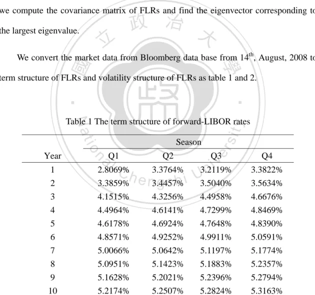
(28) Chapter. 5. Calibration. Procedure. and. Numerical analysis. Ultimately, in order to carry out the setting of one factor LMM, we implement the. 政治大 the numerical effects of pricing the two products for the model parameters in chapter 4 立 principal component analysis to a suitable covariance matrix of the FLRs, and examine. 5.1 parameters setting and calibration procedure. Nat. sit. y. ‧. ‧ 國. LMM.. 學. between Monte Carlo method and approximate formulas method in framework of. er. io. In our model, an endogenous correlation structure is set to fit swaptions if yield. al. n. iv n C calibrate market data in two stages.hThe e nfirst h i isUbootstrapping the term structure g cstage. curves and volatilities of FLRs are specific (cf. Hull and White, 1999). Therefore, we. and volatilities of FLRs from IRS and Caps, and the second one is calibrating from the swaption market data. We consider a full rank time homogeneous instantaneous correlation framework (cf. Rabonato, 2004) as follows. ρij = φ0 + (1 − φ0 ) exp(−φ1 i − j ) ,. (22). where ρij is the correlation coefficients between of i -th and j -th FLRs. There are. 24.

(29) some advantages in such setting. First, it carries out nonnegative definite correlation matrix. Second, relatively small movements in the ρij cause relatively small changes in φ0 and φ1 . Finally, the numeric of correlation between two FLRs tend to diminish as the distance of their maturity increase. In this procedure of fitting the swaptions, we employ the Rebonato swaption formula (cf. Rebonato, 2004) to match market swaption volatility under LMM.Finally, we compute the covariance matrix of FLRs and find the eigenvector corresponding to the largest eigenvalue.. 立. 政治大. ‧ 國. 學. We convert the market data from Bloomberg data base from 14th, August, 2008 to term structure of FLRs and volatility structure of FLRs as table 1 and 2.. ‧. Nat. 3.3859% 4.1515% 4.4964% 4.6178% 4.8571% 5.0066% 5.0951% 5.1628% 5.2174%. Q2. sit. Season. er. a Q1 l C 2.8069% h. n. 1 2 3 4 5 6 7 8 9 10. io. Year. y. Table 1 The term structure of forward-LIBOR rates. Q3. Q4. 4.4958% 4.7299% 4.7648% 4.9911% 5.1197% 5.1883% 5.2396% 5.2824%. 3.3822% 3.5634% 4.6676% 4.8469% 4.8390% 5.0591% 5.1774% 5.2357% 5.2794% 5.3163%. iv 3.3764% 3.2119% n e n3.4457% g c h i U3.5040% 4.3256% 4.6141% 4.6924% 4.9252% 5.0642% 5.1423% 5.2021% 5.2507%. 25.

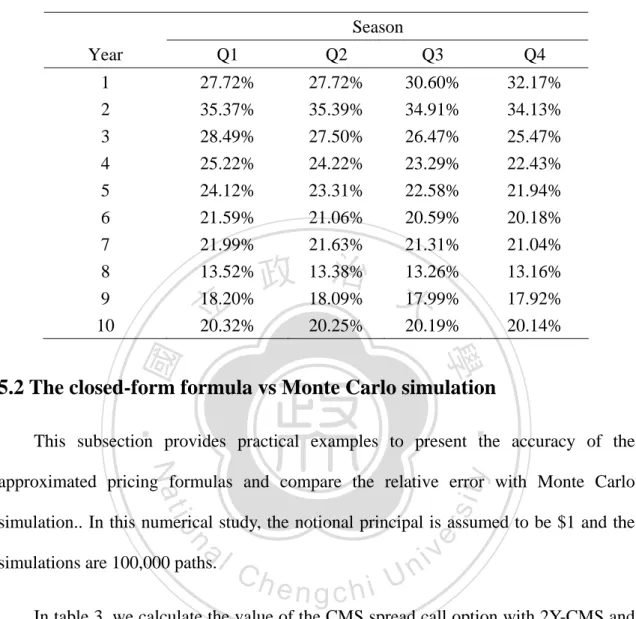
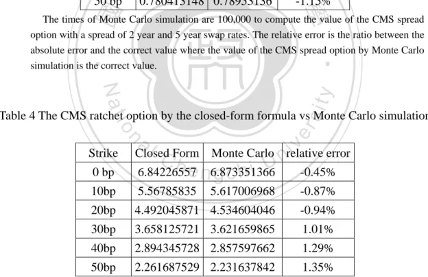
(30) Table 2 The volatilitiy structure of forward-LIBOR rates Season Year. Q1. Q2. Q3. Q4. 1 2 3 4 5 6 7 8 9 10. 27.72% 35.37% 28.49% 25.22% 24.12% 21.59% 21.99% 13.52% 18.20% 20.32%. 27.72% 35.39% 27.50% 24.22% 23.31% 21.06% 21.63% 13.38% 18.09% 20.25%. 30.60% 34.91% 26.47% 23.29% 22.58% 20.59% 21.31% 13.26% 17.99% 20.19%. 32.17% 34.13% 25.47% 22.43% 21.94% 20.18% 21.04% 13.16% 17.92% 20.14%. 立. 政治大. ‧ 國. 學. 5.2 The closed-form formula vs Monte Carlo simulation. ‧. This subsection provides practical examples to present the accuracy of the. y. Nat. io. sit. approximated pricing formulas and compare the relative error with Monte Carlo. n. al. er. simulation.. In this numerical study, the notional principal is assumed to be $1 and the simulations are 100,000 paths.. Ch. engchi. i Un. v. In table 3, we calculate the value of the CMS spread call option with 2Y-CMS and 5Y-CMS by Monte Carlo simulation and the closed form formula. The relative error is the ratio between the absolute error and the correct value. The relative errors are very small for the CMS spread options with many strikes. In table 4, we calculate the value of the CMS ratchet call option by Monte Carlo simulation and the closed form formula. Similarly, the relative errors are also very small for the CMS ratchet options with many strikes. This is to say, the approximated formulas of CMS spread options and CMS. 26.

(31) ratchet options are sufficient accurate by comparing with Monte Carlo simulations and are worth recommending for practical implementing.. Table 3 The CMS spread option with 2Y-CMS and 5Y-CMS by the closed-form formula vs Monte Carlo simulation Strike. Closed Form Monte Carlo relative error. 0 bp. 12.45731285 12.4436535. 0.11%. 10 bp. 10.0105815 9.98250304. 0.28%. 20 bp. 治政 5.12505085 5.153084696 大 2.831834454 2.81075685 立. 0.37%. 0.780413148 0.78953136. -1.15%. 7.564367352 7.53664619. 30 bp 40 bp. ‧ 國. 0.75%. 學. 50 bp. 0.55%. ‧. The times of Monte Carlo simulation are 100,000 to compute the value of the CMS spread option with a spread of 2 year and 5 year swap rates. The relative error is the ratio between the absolute error and the correct value where the value of the CMS spread option by Monte Carlo simulation is the correct value.. sit. y. Nat. n. al. er. io. Table 4 The CMS ratchet option by the closed-form formula vs Monte Carlo simulation Strike. Ch. i Un. v. Closed Form Monte Carlo relative error. e n6.873351366 gchi. 0 bp. 6.84226557. -0.45%. 10bp. 5.56785835. 5.617006968. -0.87%. 20bp. 4.492045871 4.534604046. -0.94%. 30bp. 3.658125721 3.621659865. 1.01%. 40bp. 2.894345728 2.857597662. 1.29%. 50bp. 2.261687529 2.231637842. 1.35%. The times of Monte Carlo simulation are 100,000 to compute the mean value of the CMS ratchet options. The relative error is the ratio between the absolute error and the correct value where the value of the CMS ratchet option by Monte Carlo simulation is the correct value. The computational time of Monte Carlo simulation is about 600 seconds, and the computational time of the closed-form formula is about one second.. 27.

(32) 5.3 Delta Hedge Delta hedge is the popular sensitive analysis. Traditionally, the delta for the CMS product under the LMM is practiced by computing buckets to the market rates. However, it is time-consuming and unstable due to the Monte Carlo simulation. In this paper, we provide an efficient delta hedging for the CMS product. Theorem 1 Under the condition in the lemma (4.1), let. 政治大. F (Y1 (0), Y2 (0)) = E P (δ a1Y1 (T1 ) − δ a2Y2 (T2 ) − δ K ). 立. +. be the spread option, then the delta of spread option with two reference rates can be. ‧ 國. 學. divided into four case as follow.. T1 μ1 ( t ) dt ∂F = δ a1e ∫0 ( N ( sign( g ( x* ))δ d2,1 ) − sign( g ( x* ))δ N (d1,1 ) ) , ∂Y1 (0). y. er. sit. T2 μ 2 ( t ) dt ∂F = −δ a2 e ∫0 N ( sign( g ( x* ))δ d 2,2 ) − sign( g ( x* ))δ N (d1,2 ) ) . ( ∂Y2 (0). io. Δδ2 =. Nat. Δ1δ =. ‧. Case 1: g ( x) has two real roots x1 and x2 with x1 < x* < x2 ,. n. al. i Un. Case 2 : g ( x) has unique real root x2 with x* < x2 ,. Ch. (. engchi. ). v. ∂F T Δ1 = = δ a1 exp ∫0 1 μ1 (t )dt ⎡⎣ N (δ sign( g ( x*))d 2,1 ) ⎤⎦ , ∂Y1 (0) δ. Δδ2 =. (. ). ∂F T = −δ a2 exp ∫0 2 μ2 (t )dt ⎡⎣ N (δ sign( g ( x*)d 2,2 ) ⎤⎦ . ∂Y2 (0). Case 3: g ( x) has unique real root x1 with x1 < x* ,. ( ∫ μ (t )dt ) N (−sign( g ( x ))δ d ) , ∂F = = −δ a exp ( ∫ μ (t )dt ) e ∫ N (− sign( g ( x ))δ d ∂Y (0). Δ1δ = Δδ2. ∂F = δ a1 exp ∂Y1 (0). T1. *. 1. 0. 1,1. T2. T2. 2. 0. 0. 2. μ2 ( t ) dt. *. 1,2. 2. 28. )..

(33) Case 4: g ( x) has no roots, T1. Δ1δ = sign( g ( x* ))e ∫0. μ1 ( t ) dt. T2. Δδ2 = sign( g ( x* ))a2 e ∫0. I{δ =sign ( g ( x* ))} ,. μ2 ( t ) dt. I{δ =sign ( g ( x* ))} .. In the theorem 5.1 and Lemma 4.1, we see the spread option can be decomposition to. E P (δ a1Y1 (T1 ) − δ a2Y2 (T2 ) − δ K ). 立. +. 政治大. = Y1 (0)Δ1δ + Y2 (0)Δδ2 − δ K ( N ( sign( g ( x* ))δ x2 ) − sign( g ( x* ))δ N ( x1 ) ) .. ‧ 國. 學. Analogous to the delta of BS formula, it means that we can hedge the option by. ‧. purchasing Δ1δ and Δδ2 units underlying assets respectively. This manner supplies two. y. Nat. er. io. sit. advantages. First, it is more efficiently than Monte Carlo method for computing. Second, different from the bucket method, the market parameters exploited to hedge only. n. al. Ch. i Un. v. depends on underlying assets. It can reduce the hedging cost while we wait to hedge CMS products.. engchi. 29.

(34) Chapter 6 Conclusions. In the previous research, the CMS derivatives are almost valued by the Monte Carlo simulation under the LMM. In this paper, also based on a LMM framework, we develop the approximated dynamics of the FSR and provide the approximated. 政治大 generally, some CMS products can be derived with the approximated dynamics of the 立 closed-form formulas for the CMS spread options and CMS ratchet options. More. ‧ 國. 學. swap rate.. By using the approximated valuation formulas, there are many applications for the. ‧. CMS products. CMS products can be used as ancillary instruments for interest rate. y. Nat. sit. swaps to enhance the profit from a change in the spread between two interest rate swaps. n. al. er. io. or to lock the current spread and manage interest rate risk. Besides, different from the. i Un. v. bucket hedge, it provides a way of hedging the CMS products exactly matching the. Ch. engchi. DV01 of IRS which reduces sufficiently the complicated computing. Finally, the approximated formulas of the CMS spread options are sufficiently accurate when compared with the Monte Carlo simulations and are worth practical implementing.. 30.

(35) Reference Brace, A., Dun, T. A., and Barton, G., (1998). “Toward a central interest rate model.” in Handbooks in Mathematical Finance, Topics in Option Pricing, Interest Rates and Risk Management, Cambridge University Press. Brace, A., Gatarek, D., and Musiela, M., (1997). “The Market Model of Interest Rate Dynamics.” Mathematical Finance 7, 127-155. Brigo, D., and Mercurio, F., (2006). Interest Rate Models: Theory and Practice. Second Edition, Springer Verlag. Galluccio, S., and Hunter, C., (2004). “The co-initial swap market model,” Economic Notes 33, 209-232.. 立. 政治大. ‧ 國. 學. Heath, D., Jarrow, R., Merton, A., (1992). “Bond Pricing and the Term Structure of Interest Rate: A new Methodology for Contingent claims Valuation”, Economitrica, 60, 77-105. ‧. Hunter, C. J., Jackel, P. and Joshi, M. S., (2001). “Drift approximations in a forward-rate-based LIBOR market model,” Risk Magazine 14.. y. Nat. sit. al. er. io. Hull, J., and White, A., (1999). “Forward rate volatilities, swap rate volatilities, and the implementation of the LIBOR market model,” Journal of Fixed Income 10, 46-62.. v. n. Jamshidian, F., (1997). “LIBOR and swap market model and measure,” Finance and Stochastics 1, 293-330.. Ch. engchi. i Un. Mercurio, F., and Pallavicini, A., (2005). “Mixing Gaussian models to price CMS derivatives,” Working paper. Musiela, M. and Rutkowski, M., (1997). “Continuous-time term structure models:a forward measure approach.” Finance Stochast 1, 261-291 Rebonato, R., (2004) Volatility and Correlation: The Perfect Hedger and the Fox. Second Edition. John. Wiley & Sons, New York.. 31.

(36) Appendix A: Proof of Lemma 4.1. We first consider expectation in Lemma 1. E P (δ a1Y1 (T1 ) − δ a2Y2 (T2 ) − δ K ) . +. Using the properties of Geometric Brownian Motion, it can be represented to. E P ⎡δ a1Y1 (0) exp ⎢⎣. (∫. −δ a2Y2 (0) exp =∫. ∞. −∞. (δβ e. ∞. γ 1 T1 x. 1. (δ g ( x) ) −∞. =∫. +. ( μ1 (t ) - 0.5σ 12 (t ))dt + ∫0 σ 1 (t )dW (t ). T1. T1. 0. (∫. T2. 0. − δβ 2 e. ) ). ( μ 2 (t ) - 0.5σ 2 2 (t ))dt + ∫0 σ 2 (t ) dW (t ) − δ K ⎤ ⎥⎦ T2. γ 2 T2 x. ). +. − δ K n( x)dx. 立. n( x)dx .. +. 政治大. ‧ 國. 學. Thus, we are interesting to find region in the range of δ g ( x) which is nonnegative. Next, we search the roots of δ g ( x) . First, differential g ( x) with respect to x to obtain. − β 2γ 2 T2 eγ 2. T2 x. γ1 T1 x. *. = β 2γ 2. d 2 g ( x* ) γ = β1γ 1e 1 dx 2. T1 x*. TC eh. sit. y. al. .. er. γ 2 T2 − γ 1 T1. n. we have. , and find that g ( x) has unique critical point. ln( β1γ 1 T1 ) − ln( β 2γ 2 T2 ). io. x* =. Let η = β1γ 1 T1 e. ‧. T1 x. Nat. dg ( x) = β1γ 1 T1 eγ1 dx. iv n compute the second derivative at e>n0gand chi U. γ 2 T2 x*. 2. γ 1 T1 − β 2γ 2 eγ. 2. T2 x*. x* ,. γ 2 T2 = η (γ 1 T1 − γ 2 T2 ) .. d 2 g ( x* ) > 0 iff γ 1 T1 > γ 2 T2 . Hence g ( x) has unique min value or max value. dx 2 So there are at most two roots of δ g ( x) . We compute the expectation in Lemma 1 in. Then. accordance with roots of g . Define 2. x − 1 1 − 12 x2 e 2T . g c ( x) = max( g ( x), 0) , g p ( x) = max(− g ( x), 0) , n( x) = e , nT ( x) = 2π T 2π. 32.

(37) Case 1: g ( x) has two real roots x1 , x2 with x1 < x* < x2 . If g ( x* ) < 0 , then g ( x) has nonnegative value on (−∞, x1 ] ∪ [ x2 , ∞) and. g ( x) has nonpositive value on [ x1 , x2 ] .. ∫. ∞. ∫. x1. x1. ∞. −∞. x2. g c ( x)n( x)dx = ∫ g ( x)n( x)dx + ∫ g ( x)n( x)dx ,. −∞. T1 x1. g ( x)n( x)dx = ∫. −∞. −∞. = β1e. 1 2 γ 1 T1 2. 1. −∞. 1. N (d1,1 ) − β 2e. 1 2 γ 2 T2 2. 立. g ( x)n( x)dx. ∞. −∞. 2. 政治大 T . 2. ‧ 國. x2. 2. 學. ∫. x1. β 2eγ x nT ( x)dx − K ∫ n( x)dx. N (d1,2 ) − KN ( x1 ) ,. where d1,1 = x1 − γ 1 T1 , d1,2 = x1 − γ 2 ∞. T2 x1. β1eγ x nT ( x)dx − ∫. x2. = ∫ g ( x)n( x)dx − ∫ g ( x)n( x)dx. 1 2 γ 2 T2 ⎡ 12 γ12T1 ⎤ − K − ⎢ β1e N (d 2,1 ) − β 2 e 2 N (d 2,2 ) − KN ( x2 ) ⎥ , ⎣ ⎦. y. − β2e. 1 2 γ 2 T2 2. sit. 1 2 γ 1 T1 2. Nat. = β1e. −∞. ‧. −∞. er. io. where d 2,1 = x2 − γ 1 T1 , d 2,2 = x2 − γ 2 T2 .. al. iv n C β ei U (1 + N (d (1 + N (d )h− eN (nd g) )c− h. n. ∫. ∞. −∞. g c ( x)n( x)dx = β1e. 1 2 γ 1 T1 2. 1 2 γ 2 T2 2. 1,1. 2,1. 2. 1,2. ) − N (d 2,2 ) ). − K (1 + N ( x1 ) − N ( x2 ) ) = β1e. 1 2 γ 1 T1 2. ( N (d. 1,1. ) + N (− d 2,1 ) ) − β 2 e. 1 2 γ 2 T2 2. − K ( N ( x1 ) + N (− x2 ) ) .. ∫. ∞. −∞. ∞. ∞. −∞. −∞. g p ( x)n( x)dx = ∫ g c ( x)n( x)dx − ∫ g ( x)n( x)dx ,. 33. ( N (d. 1,2. ) + N (− d 2,2 ) ).

(38) ∫. ∞. −∞. x2. g p ( x)n( x)dx = − ∫ g ( x)n( x)dx x1. x2. x1. −∞. −∞. = − ∫ g ( x)n( x)dx + ∫ g ( x)n( x)dx = β1e. 1 2 γ 1 T1 2. ( N (d. 1,1. ) − N (d 2,1 ) ) − β 2 e. 1 2 γ 2 T2 2. ( N (d. 1,2. ) − N (d 2,2 ) ). − K ( N ( x1 ) − N ( x2 ) ) . T1. E P ( a1Y1 (T1 ) − a2Y2 (T2 ) − K ) = a1Y1 (0)e ∫0 +. T2. − a2Y2 (0)e ∫0. μ2 ( t ) dt. μ1 ( t ) dt. ( N (− d. 2,2. ( N (− d. 2,1. ) + N (d1,1 ) ). ) + N (d1,2 ) ) − K ( N (− x2 ) + N ( x1 ) ) .. 治政 ∫ E ( K − a Y (T ) + a Y (T ) ) = −a Y (0)e N (d ( N (d ) −大立 T1. +. 1 1. P. 1. 2 2. 0. 2. T2. μ 2 ( t ) dt. 2,1. ( N (d. 2,2. T1. +. 2,2. 2,1. ) + δ N (d1,1 ) ). ) + δ N (d1,2 ) ) − δ K ( N (−δ x2 ) + δ N ( x1 ) ) . (A1). sit. Nat. ( N (−δ d. ( N (−δ d. y. μ 2 ( t ) dt. μ1 ( t ) dt. ‧. T2. )). ) − N (d1,2 ) ) + K ( N ( x2 ) − N ( x1 ) ) .. E P ( a1δ Y1 (T1 ) − a2δ Y2 (T2 ) − δ K ) = δ a1Y1 (0)e ∫0 −δ a2Y2 (0)e ∫0. 1,1. 學. + a2Y2 (0)e ∫0. ‧ 國. μ1 ( t ) dt. 1 1. n. al. er. io. If g ( x* ) > 0 , then g ( x) has nonnegative value on [ x1 , x2 ] and g ( x) has nonpositive value on (−∞, x1 ] ∪ [ x2 , ∞) .. ∫ =∫. ∞. −∞. x2. x1. = β1e. ∫. ∞. −∞. g c ( x)n( x)dx. Ch. engchi. i Un. v. g ( x)n( x)dx 1 2 γ 1 T1 2. ( N (d. 2,1. ) − N (d1,1 ) ) − β 2 e. 1 2 γ 2 T2 2. ( N (d. x1. ∞. −∞. x2. 2,2. ) − N (d1,2 ) ) − K ( N ( x2 ) − N ( x1 ) ) .. g p ( x)n( x)dx = − ∫ g ( x)n( x) dx − ∫ g ( x)n( x)dx 1. = β1e 2. γ 12T1. ( − N (− d. 1. 2 2,1 ) − N ( d1,1 ) ) − β 2 e. − K ( − N (− x2 ) − N ( x1 ) ) .. 34. γ 2 2T2. ( − N (− d. 2,2. ) − N (d1,2 ) ).

(39) T1. E P ( a1Y1 (T1 ) − a2Y2 (T2 ) − K ) = a1Y1 (0)e ∫0 +. T2. − a2Y2 (0)e ∫0. μ 2 ( t ) dt. ( N (d. 2,2. T1. +. T2. μ2 ( t ) dt. ( − N (−d. 2,2. ( N (δ d. μ 2 ( t ) dt. 2,1. ) − N (d1,1 ) ). ) − N (d1,2 ) ) − K ( − N (− x2 ) − N ( x1 ) ) . T1. +. T2. ) − N (d1,1 ) ). ( − N (− d. μ1 ( t ) dt. E P (δ a1Y1 (T1 ) − δ a2Y2 (T2 ) − δ K ) = δ a1Y1 (0)e ∫0 −δ a2Y2 (0)e ∫0. 2,1. ) − N (d1,2 ) ) − K ( N ( x2 ) − N ( x1 ) ) .. E P ( K − a1Y1 (T1 ) + a2Y2 (T2 ) ) = a1Y1 (0)e ∫0 − a2Y2 (0)e ∫0. ( N (d. μ1 ( t ) dt. 2,2. μ1 ( t ) dt. ( N (δ d. 2,1. ) − δ N (d1,1 ) ). 政治大. ) − δ N (d1,2 ) ) − K ( N (δ x2 ) − δ N ( x1 ) ) .. 立. (A2). We combine (A1) and (A2) to acquire. *. 2,1. ( N (sign( g ( x ))δ d. ) − sign( g ( x* ))δ N (d1,1 ) ). *. Nat. 2,2. ) − sign( g ( x* ))δ N (d1,2 ) ). y. μ2 ( t ) dt. ( N (sign( g ( x ))δ d. n. er. io. sit. −δ K ( N ( sign( g ( x* ))δ x2 ) − sign( g ( x* ))δ N ( x1 ) ) .. al. ‧. T2. −δ a2Y2 (0)e ∫0. μ1 ( t ) dt. ‧ 國. T1. = δ a1Y1 (0)e ∫0. +. 學. E P (δ a1Y1 (T1 ) − δ a2Y2 (T2 ) − δ K ). Ch. engchi. i Un. v. Case 2: g ( x) has unique real root x2 more than x* .. If g ( x* ) < 0 , then g ( x) has nonnegative value on [ x2 , ∞) and. g ( x) has nonpositive value on (−∞, x2 ] .. ∫. ∞. −∞. ∞. g c ( x)n( x)dx = ∫ g ( x)n( x)dx x2. = β1e. = β1e. 1 2 γ 1 T1 2. (1 − N (d ) ) − β e 2,1. 1 2 γ 1 T1 2. N (− d 2,1 ) − β 2 e. 1 2 γ 2 T2 2. 2. 1 2 γ 2 T2 2. (1 − N (d ) ) − K (1 − N ( x ) ) 2,2. N (− d 2,2 ) − KN (− x2 ) .. 35. 2.

(40) ∫. ∞. x2. −∞. g p ( x)n( x)dx = − ∫ g ( x)n( x)dx −∞. 1 2 γ 2 T2 ⎡ 1 γ12T1 ⎤ = − ⎢ β1e 2 N (d 2,1 ) − β 2 e 2 N (d 2,2 ) − KN ( x2 ) ⎥ ⎣ ⎦. = KN ( x2 ) + β 2 e. E P ( a1Y1 (T1 ) − a2Y2 (T2 ) − K ) μ1 ( t ) dt. T2. N (− d 2,1 ) − a2Y2 (0)e ∫0 +. 立. μ1 ( t ) dt. 政治大 T1. N (d 2,2 ) − a1Y1 (0)e ∫0. E P (δ a1Y1 (T1 ) − δ a2Y2 (T2 ) − δ K ) T1. N (− d 2,2 ) − KN (− x2 ) ,. μ1 ( t ) dt. N (d 2,1 ) .. +. T2. μ2 ( t ) dt. N (−δ d 2,2 ) − δ KN (−δ x2 ) .. (A3). sit. Nat. N (−δ d 2,1 ) − δ a2Y2 (0)e ∫0. ‧. ‧ 國. = KN ( x2 ) + a2Y2 (0)e ∫. μ 2 ( t ) dt. 學. T2 μ 2 ( t ) dt 0. N (d 2,1 ) .. +. E P ( K − a1Y1 (T1 ) + a2Y2 (T2 ) ). = δ a1Y1 (0)e ∫0. N (d 2,2 ) − β1e. 1 2 γ 1 T1 2. y. T1. = a1Y1 (0)e ∫0. 1 2 γ 2 T2 2. n. al. er. io. If g ( x* ) > 0 , then g ( x) has nonnegative value on (−∞, x2 ] and. g ( x) has nonpositive value on [ x2 , ∞) .. ∫. ∞. −∞. x2. g c ( x)n( x)dx = ∫ g ( x)n( x)dx 1. ∞. −∞. engchi. i Un. v. −∞. = β1e 2. ∫. Ch. γ 12T1. 1. N (d 2,1 ) − β 2 e 2. γ 22T2. N (d 2,2 ) − KN ( x2 ) .. ∞. g p ( x)n( x)dx = − ∫ g ( x)n( x)dx x2. = β1e. 1 2 γ 1 T1 2. = − β1e. N (d 2,1 ) − β 2 e. 1 2 γ 1 T1 2. 1 2 γ 2 T2 2. N (− d 2,1 ) + β 2 e. 1 2 γ 2 T2 ⎡ 12 γ12T1 ⎤ − β 2e 2 − K⎥ N (d 2,2 ) − KN ( x2 ) − ⎢ β1e ⎣ ⎦. 1 2 γ 2 T2 2. 36. N (−d 2,2 ) + KN (− x2 ) ..

(41) E P ( a1Y1 (T1 ) − a2Y2 (T2 ) − K ) T1. = a1Y1 (0)e ∫0. μ1 ( t ) dt. +. T2. N (d 2,1 ) − a2Y2 (0)e ∫0. E P ( K − a1Y1 (T1 ) + a2Y2 (T2 ) ) T2. = KN (− x2 ) + a2Y2 (0)e ∫0. μ2 ( t ) dt. T1. μ1 ( t ) dt. N (d 2,2 ) − KN ( x2 ) ,. +. T1. N (− d 2,2 ) − a1Y1 (0)e ∫0. E P (δ a1Y1 (T1 ) − δ a2Y2 (T2 ) − δ K ) = δ a1Y1 (0)e ∫0. μ 2 ( t ) dt. μ1 ( t ) dt. N (− d 2,1 ) .. +. (δ d ) − δ KN (δ x ) . 政 N治大 T2. N (δ d 2,1 ) − δ a2Y2 (0)e ∫0. 立. μ 2 ( t ) dt. 2,2. 2. We combine (A3) and (A4) to acquire. ‧ 國 T1. μ1 ( t ) dt. T2. μ2 ( t ) dt. −δ a2Y2 (0)e. ∫0. N ( sign( g ( x* ))δ d 2,1 ). ‧. = δ a1Y1 (0)e ∫0. +. 學. E P (δ a1Y1 (T1 ) − δ a2Y2 (T2 ) − δ K ). N ( sign( g ( x* ))δ d 2,2 ). y. Nat. n. er. io. al. sit. −δ KN ( sign( g ( x* ))δ x2 ) .. Ch. engchi. Case 3: g ( x) has unique real root x1 less than x* .. i Un. v. If g ( x* ) < 0 , then g ( x) has nonnegative value on (−∞, x1 ] and. g ( x) has non positive value on [ x1 , ∞) .. ∫. ∞. −∞. x1. g c ( x)n( x)dx = ∫ g ( x)n( x)dx −∞. = β1e. ∫. ∞. −∞. 1 2 γ 1 T1 2. N (d1,1 ) − β 2 e. 1 2 γ 2 T2 2. N (d1,2 ) − KN ( x1 ) ,. ∞. g p ( x)n( x)dx = − ∫ g ( x)n( x)dx x1. 37. (A4).

(42) 1. = β1e 2. γ 12T1. 2 1,1 ) − 1) − β 2 e. E P ( a1Y1 (T1 ) − a2Y2 (T2 ) − K ) T1. = a1Y1 (0)e ∫0. μ1 ( t ) dt. T1. T1. μ1 ( t ) dt. T1. 1,2. ) − 1) − K ( N ( x1 ) − 1) ,. μ1 ( t ) dt. N (d1,2 ) − KN ( x1 ) ,. T2. N (− d1,1 ) + a2Y2 (0)e ∫0. μ 2 ( t ) dt. N (− d1,2 ) + KN (− x1 ) .. 政治大. +. 立. T2. N (δ d1,1 ) − δ a2Y2 (0)e ∫0. μ 2 ( t ) dt. N (δ d1,2 ) − δ KN (δ x1 ) .. 學. ‧ 國. μ1 ( t ) dt. ( N (d. +. E P (δ a1Y1 (T1 ) − δ a2Y2 (T2 ) − δ K ) = δ a1Y1 (0)e ∫0. γ 2 2T2. +. N (d1,1 ) − a2Y2 (0)e ∫0. E P ( K − a1Y1 (T1 ) + a2Y2 (T2 ) ) = − a1Y1 (0)e ∫0. 1. ( N (d. If g ( x* ) > 0 , then g ( x) has nonnegative value on [ x1 , ∞) and. ∞. g c ( x)n( x)dx = ∫ g ( x)n( x)dx. −∞. gp. y. N (−d1,1 ) − β 2 e. al. 1 2 γ 2 T2 2. n. ∫. ∞. io. = β1e. 1 2 γ 1 T1 2. sit. x1. N (− d1,2 ) − KN (− x1 ) ,. er. ∞. −∞. Nat. ∫. ‧. g ( x) has nonpositive value on (−∞, x1 ] .. ni ( x)n( x)dx = − ∫ g ( x)n( x)dxC h U engchi x1. v. −∞. 1 2 γ 2 T2 ⎡ 1 γ12T1 ⎤ = − ⎢ β1e 2 N (d1,1 ) − β 2 e 2 N (d1,2 ) − KN ( x1 ) ⎥ ⎣ ⎦ 1. = KN ( x1 ) + β 2 e 2. E P ( a1Y1 (T1 ) − a2Y2 (T2 ) − K ) T1. = a1Y1 (0)e ∫0. μ1 ( t ) dt. γ 22T2. γ 12T1. N (d1,1 ) .. +. T2. N (− d1,1 ) − a2Y2 (0)e ∫0. E P ( K − a1Y1 (T1 ) + a2Y2 (T2 ) ). 1. N (d1,2 ) − β1e 2. μ2 ( t ) dt. N (− d1,2 ) − KN (− x1 ) ,. +. 38. (A5).

(43) T2. = KN ( x1 ) + a2Y2 (0)e ∫0. μ 2 ( t ) dt. T1. N (d1,2 ) − a1Y1 (0)e ∫0. E P (δ a1Y1 (T1 ) − δ a2Y2 (T2 ) − δ K ) T1. = δ a1Y1 (0)e ∫0. μ1 ( t ) dt. μ1 ( t ) dt. N (d1,1 ) .. +. T2. N (−δ d1,1 ) − δ a2Y2 (0)e ∫0. μ2 ( t ) dt. N (−δ d1,2 ) − δ KN (−δ x1 ) .. (A6). We combine (A5) and (A6) to acquire. E P (δ a1Y1 (T1 ) − δ a2Y2 (T2 ) − δ K ) T1. μ1 ( t ) dt. T2. μ2 ( t ) dt. = δ a1Y1 (0)e ∫0 −δ a2Y2 (0)e. ∫0. +. N (− sign( g ( x* ))δ d1,1 ). 立. 政治大. N (− sign( g ( x* ))δ d1,2 ). −δ KN (− sign( g ( x* ))δ x1 ) .. ‧. ‧ 國. 學. Case 4: g ( x) has no real root.. −∞. ∞. y. sit. al. er. ∫. ∞. g c ( x)n( x)dx = 0 ,. n. ∞. −∞. io. ∫. Nat. If g ( x* ) < 0 , then g ( x) < 0 for all x .. 1. g p ( x)n( x)dx = ∫ − g ( x)n( x)dx = K − β1e 2 −∞. Ch. E P ( a1Y1 (T1 ) − a2Y2 (T2 ) − K ) = 0 , +. T1. +. E P (δ a1Y1 (T1 ) − δ a2Y2 (T2 ) − δ K ). i U n.. 1. + β 2e 2. engchi. E P ( K − a1Y1 (T1 ) + a2Y2 (T2 ) ) = K − a1Y1 (01 )e ∫0 +. γ 12T1. μ1 ( t ) dt. γ 2 2T2. T2. + a2Y2 (0)e ∫0. ∫. −∞. ∞. T. 1. g c ( x)n( x)dx = ∫ g ( x)n( x)dx = β1e 2 −∞. μ 2 ( t ) dt. .. 1 2 μ1 ( t ) dt μ2 ( t ) dt ⎛ ⎞ = − ⎜ a1Y1 (01 )e ∫0 − a2Y2 (0)e ∫0 − K ⎟ I{δ =−1} . (A7) ⎝ ⎠. T. If g ( x* ) > 0 , then g ( x) > 0 for all x . ∞. v. γ 12T1. 1. − β 2e 2. 39. γ 22T2. −K ,.

(44) ∫. ∞. −∞. g p ( x)n( x)dx = 0 . T1. E P ( a1Y1 (T1 ) − a2Y2 (T2 ) − K ) = a1Y1 (01 )e ∫0 +. T2. − a2Y2 (01 )e ∫0. μ1 ( t ) dt. μ 2 ( t ) dt. −K ,. E P ( K − a1Y1 (T1 ) + a2Y2 (T2 ) ) = 0 . +. 1 2 μ1 ( t ) dt μ 2 ( t ) dt + ⎛ ⎞ − a2Y2 (0)e ∫0 − K ⎟ I{δ =1} E P (δ a1Y1 (T1 ) − δ a2Y2 (T2 ) − δ K ) = ⎜ a1Y1 (01 )e ∫0 ⎝ ⎠. T. T. We combine (A7) and (A8) to acquire. E P (δ a1Y1 (T1 ) − δ a2Y2 (T2 ) − δ K ). +. 政治⎞ 大 − a Y (0 )e ∫ −K⎟I 立 ⎠. ⎛ = sign( g ( x* )) ⎜ a1Y1 (01 )e ∫ ⎝. T1 μ ( t ) dt 0 1. T2. 0. 2 2. μ 2 ( t ) dt. {δ = sign ( g ( x* ))}. 1. .. ‧. ‧ 國. 學. n. er. io. sit. y. Nat. al. Ch. engchi. 40. i Un. v. . (A8).

(45) Appendix B.1: Leibniz’s rule Let gu ( y1 , y2 ), gl ( y1 , y2 ) ∈ C1 (. 2. ) and h(.,.; x) ∈ C1 (. 2. ) for any x ,. with respective x , for any y1 , y2 ∈. h( y1 , y2 ; x) is integrable on. .. Then we have the following some case. Case 1: Let F ( y1 , y2 ) = ∫. gu ( y1 , y2 ). gl ( y1 , y2 ). h( y1 , y2 ; x)dx and h, gu , gl satisfy. h( y1 , y2 ; gu ( y1 , y2 )) = h( y1 , y2 ; gl ( y1 , y2 )) = 0 . ∂g ( y , y ) ∂g ( y , y ) ∂F ( y1 , y2 ) = h( y1 , y2 ; gu ( y1 , y2 )) u 1 2 − h( y1 , y2 ; gl ( y1 , y2 )) l 1 2 ∂yi ∂yi ∂yi. gu ( y1 , y2 ). gl ( y1 , y2 ). ∂h( y1 , y2 ; x) dx for i = 1, 2 . ∂yi. gu ( y1 , y2 ). Nat. Case 2: let F ( y1 , y2 ) = ∫. −∞. h( y1 , y2 ; x)dx and. y. =∫. io. h, gu satisfy h( y1 , y2 ; gu ( y1 , y2 )) = 0 .. n. al. ‧. ‧ 國. gl ( y1 , y2 ). 立. ∂h( y1 , y2 ; x) dx ∂yi. sit. gu ( y1 , y2 ). 學. +∫. 政治大. er. Then. i Un. v. gu ( y1 , y2 ) ∂h( y , y ; x ) ∂g ( y , y ) ∂F ( y1 , y2 ) 1 2 =∫ dx + h( y1 , y2 ; gu ( y1 , y2 )) u 1 2 Then −∞ ∂yi ∂yi ∂yi. =∫. gu ( y1 , y2 ). −∞. Case 3 : Let F ( y1 , y2 ) = ∫. Ch. engchi. ∂h( y1 , y2 ; x) dx for i = 1, 2 . ∂yi. ∞. gl ( y1 , y2 ). h( y1 , y2 ; x)dx and. h, gl satisfy h( y1 , y2 ; gl ( y1 , y2 )) = 0 . Then. ∞ ∂g ( y , y ) ∂F ( y1 , y2 ) ∂h( y1 , y2 ; x) =∫ dx − h( y1 , y2 ; g l ( y1 , y2 )) l 1 2 gl ( y1 , y2 ) ∂yi ∂yi ∂yi. 41.

(46) =∫. ∞. gl ( y1 , y2 ). ∂h( y1 , y2 ; x) dx for i = 1, 2 . ∂yi. 立. 政治大. ‧. ‧ 國. 學. n. er. io. sit. y. Nat. al. Ch. engchi. 42. i Un. v.

(47) Appendix B.2: Proof of theorem 5.1. Under the setting in Lemma 4.1, we rewrite the spread option to. ∫. ∞. −∞. (δ Y (0)ψ exp (γ 1. 1. where ψ i = ai exp. Let. ). (. ). ). +. T1 x − δ Y2 (0)ψ 2 exp γ 2 T2 x − δ K n( x)dx ,. 1. ( ∫ (μ (t) - 0.5σ Ti. i. 0. (. 2. i. (t ))dt. ). for i = 1, 2 .. (. ). ) ). (. h(Y1 (0), Y2 (0); x) = Y1 (0)ψ 1 exp γ 1 T1 x − Y2 (0)ψ 2 exp γ 2 T2 x − K n( x). and calculate the derivative with respect to Y1 (0) and Y2 (0). 政治大. ( x − γ 1 T1 ) 2 γ 12T1 1 ∂h = ψ 1 exp( ) exp(− ), ∂Y1 (0) 2 2 2π. 學. ‧ 國. 立. ( x − γ 2 T2 ) 2 γ 2T ∂h 1 = −ψ 2 exp( 2 2 ) exp(− ). ∂Y2 (0) 2 2 2π. ‧. Next, we will derive the delta of spread option in case 1 under the setting in Lemma 4.1,. er. io. Suppose g ( x) has two real roots x1 , x2 with x1 < x* < x2. al. iv n C has nonnegative on (−∞, x ] ∪ [ x , ∞) h e nvalue gchi U n. If g ( x ) < 0 , then g ( x) *. sit. y. Nat. and deal with other cases in similar way.. 1. 2. and. g ( x) has nonpositive value on [ x1 , x2 ] . First , we compute the call. Let x2 = gl (Y1 (0), Y2 (0)) , x1 = gu (Y1 (0), Y2 (0)) , then ∞. x1. ∞. −∞. −∞. x2. Fc (Y1 (0), Y2 (0)) = ∫ g c ( x)n( x)dx = ∫ g ( x)n( x)dx + ∫ g ( x)n( x) dx =∫. gu (Y1 (0),Y2 (0)). =∫. gu (Y1 (0),Y2 (0)). −∞. −∞. g ( x)n( x)dx + ∫. ∞. gl (Y1 (0),Y2 (0)). h(Y1 (0), Y2 (0); x)dx + ∫. g ( x)n( x)dx. ∞. gl (Y1 (0),Y2 (0)). Using Leibniz’s rule and the characteristic 43. h(Y1 (0), Y2 (0); x)dx ..

(48) h(Y1 (0), Y2 (0); gl (Y1 (0), Y2 (0))) = h(Y1 (0), Y2 (0); gu (Y1 (0), Y2 (0))) = 0 , we have gu (Y1 (0),Y2 (0)) ∂h(Y (0), Y (0); x ) ∞ ∂Fc ∂h(Y1 (0), Y2 (0); x) 1 2 =∫ dx + ∫ dx gl (Y1 (0),Y2 (0)) ∂Y1 (0) −∞ ∂Y1 (0) ∂Y1 (0). Δ1c. = ψ 1 exp(. γ 12T1 ⎡. = ψ 1 exp(. ∞ ( x − γ 1 T1 ) 2 ( x − γ 1 T1 ) 2 ⎤ 1 1 exp(− )dx + ∫ exp(− )dx ⎥ gl (Y1 (0),Y2 (0)) 2 2 2π 2π ⎦⎥. gu (Y1 (0),Y2 (0)). )⎢ 2 ⎣⎢ ∫−∞. γ 12T1 ⎡ ) N ( gu (Y1 (0), Y2 (0)) − γ 1 T1 ) + N (− gl (Y1 (0), Y2 (0)) + γ 1 T1 ) ⎤⎦ 2 ⎣. 政治大. γ 12T1 ⎡ ) N ( x1 − γ 1 T1 ) + N (− x2 + γ 1 T1 ) ⎤⎦ = ψ 1 exp( 2 ⎣. T1. 0. ). μ1 (t )dt ⎡⎣ N (d1,1 ) + N (−d 2,1 ) ⎤⎦ ,. ‧. (∫. gu (Y1 (0),Y2 (0)) ∂h(Y (0), Y (0); x ) ∞ ∂Fc ∂h(Y1 (0), Y2 (0); x) 1 2 =∫ dx + ∫ dx g Y Y ( (0), (0)) −∞ 2 l 1 ∂Y2 (0) ∂Y2 (0) ∂Y2 (0). sit. gu (Y1 (0),Y2 (0)). al. n. )⎢ 2 ⎣⎢ ∫−∞. ∞ ( x − γ 2 T2 ) 2 ( x − γ 2 T2 ) 2 ⎤ 1 1 exp(− )dx + ∫ exp(− )dx ⎥ gl (Y1 (0),Y2 (0)) 2 2 2π 2π ⎦⎥. er. γ 2 2T2 ⎡. io. = −ψ 2 exp(. y. Nat. Δ c2 =. 2. ) ⎡⎣ N (d1,1 ) + N (− d 2,1 ) ⎤⎦. 學. = a1 exp. 立. γ 12T1. ‧ 國. = ψ 1 exp(. Ch. i Un. v. = −ψ 2 exp(. γ 2 T2 ⎡ ) N ( gu (Y1 (0), Y2 (0)) − γ 2 T2 ) + N (− gl (Y1 (0), Y2 (0)) + γ 2 T2 ) ⎤⎦ 2 ⎣. = −ψ 2 exp(. γ 2 2T2 ⎡ ) N ( x1 − γ 2 T2 ) + N (− x2 + γ 2 T2 ) ⎤⎦ 2 ⎣. = −ψ 2 exp(. = − a2 exp. 2. γ 2 2T2 2. (∫. T2. 0. engchi. ) ⎡⎣ N (d1,2 ) + N (− d 2,2 ) ⎤⎦. ). μ2 (t )dt ⎡⎣ N (d1,2 ) + N (−d 2,2 ) ⎤⎦ .. Next, consider the put. Let x1 = gl (Y1 (0), Y2 (0)) , x2 = gu (Y1 (0), Y2 (0)) , then ∞. x2. gu (Y1 (0),Y2 (0)). −∞. x1. gl (Y1 (0),Y2 (0)). Fp (Y1 (0), Y2 (0)) = ∫ g p ( x)n( x)dx = − ∫ g ( x)n( x)dx = − ∫ 44. g ( x)n( x)dx.

(49) gu (Y1 (0),Y2 (0)). = −∫. gl (Y1 (0),Y2 (0)). h(Y1 (0), Y2 (0); x)dx .. By the same way, using Leibniz’s rule and following phenomenon h(Y1 (0), Y2 (0); gl (Y1 (0), Y2 (0))) = h(Y1 (0), Y2 (0); gu (Y1 (0), Y2 (0))) = 0 , we have = −∫. gl (Y1 (0),Y2 (0)). = −ψ 1 exp(. ∂Fp. T1. 0. 立. ). μ1 (t )dt ⎡⎣ N (d 2,1 ) − N (d1,1 ) ⎤⎦ ,. gu (Y1 (0),Y2 (0)). gl (Y1 (0),Y2 (0)). γ 2 2T2 ⎡. ∂h(Y1 (0), Y2 (0); x) dx ∂Y2 (0). gu (Y1 (0),Y2 (0)). )⎢ 2 ⎣⎢ ∫gl (Y1 (0),Y2 (0)). Nat. = ψ 2 exp(. T2. )a l. ( x − γ 2 T2 ) 2 ⎤ 1 exp(− )dx ⎥ 2 2π ⎦⎥. io. (∫. 政治大. μ2 (t )dt ⎡⎣ N (d 2,2 ) − N (−d1,2 ) ⎤⎦ .. n. 0. ‧. = −∫. ∂Y2 (0). = a2 exp. (∫. ( x − γ 1 T1 ) 2 ⎤ 1 exp(− )dx ⎥ 2 2π ⎦⎥. 學. Δ 2p =. gu (Y1 (0),Y2 (0)). )⎢ 2 ⎣⎢ ∫gl (Y1 (0),Y2 (0)). ‧ 國. = − a1 exp. γ 12T1 ⎡. ∂h(Y1 (0), Y2 (0); x) dx ∂Y1 (0). Ch. y. ∂Y1 (0). gu (Y1 (0),Y2 (0)). sit. ∂Fp. er. Δ1p. i Un. engchi. v. If g ( x* ) > 0 , then g ( x) has non negative value on [ x1 , x2 ] and. g ( x) has nonpositive value on (−∞, x1 ] ∪ [ x2 , ∞) . Let x1 = gl (Y1 (0), Y2 (0)) , x2 = gu (Y1 (0), Y2 (0)) , then ∞. x2. gu (Y1 (0),Y2 (0)). −∞. x1. gl (Y1 (0),Y2 (0)). Fc (Y1 (0), Y2 (0)) = ∫ g c ( x)n( x)dx = ∫ g ( x)n( x)dx = ∫ =∫. gu (Y1 (0),Y2 (0)). gl (Y1 (0),Y2 (0)). g ( x)n( x)dx. h(Y1 (0), Y2 (0); x)dx .. Because h(Y1 (0), Y2 (0); gl (Y1 (0), Y2 (0))) = h(Y1 (0), Y2 (0); gu (Y1 (0), Y2 (0))) = 0 ,. 45.