合作式定位之低維度最小方差演算法

國 立 交 通 大 學

電信工程研究所

碩 士 論 文

合作式定位之低維度最小方差演算法

Dimension-Reduced Least-Squares Algorithms for

Cooperative Localization

研究生：李冠杰

指導教授：謝世福 教授

合作式定位之低維度最小方差演算法

Dimension-Reduced Least-Squares Algorithms for

Cooperative Localization

研 究 生：李冠杰 Student：K.C. Lee

指導教授：謝世福 Advisor：S. F. Hsieh

國 立 交 通 大 學

電信工程研究所

碩 士 論 文

A Thesis

Submitted to Institute of Electrical Engineering College of Electrical and Computer Science

National Chiao Tung University In Partial Fulfillment of the Requirements

For the Degree of Master

In

Communication Engineering July 2012

Hsinchu, Taiwan, Republic of China

i

合作式定位之低維度最小方差演算法

學生:李冠杰 指導教授:謝世福

國立交通大學電信工程研究所

中文摘要

隨著無線通訊的發展，定位的研究已成為重要的議題。近年來，藉由待測物之間彼 此相互通訊的合作式定位更是目前發展的重點。在合作式定位系統中，多個待測目標之 間額外的合作量測可以有效提升其定位的精準度；但由於待測目標的增加，因此演算法 的複雜度相較於傳統定位法更是困難許多。在諸多演算法中，高斯-牛頓法被廣泛的應 用在定位的問題中，效能也與 Cramer-Rao Lower Bound (CRLB) 相當；然而其牽涉到反 矩陣的運算，使得伴隨而來的複雜度相當高。我們試著藉由降低矩陣的維度使反矩陣的 運算量降低，進而達到降低複雜度的目標。在論文中，我們設定一個待測物為目標待測 物，並試著尋找其餘附屬待測物與目標待測物之間的位置關係，藉此來達到降低運算度 的目的，並維持其定位準確度。因此，我們提出了聯合式、平行式與序列式三種預先線 性化的方法使附屬待測物的位置座標轉化成目標待測物的線性函式。接著再利用此線性 函式使原來的多待測物問題降階成一個目標待測物的估計問題並利用低維度高斯-牛頓 法來估計。其中平行式與序列式的演算法運算複雜度順利的被簡化。另外，基於目標待 測物的位置估計的影響，我們更進一步提出目標待測物的選擇機制，進而增進定位的效 能；另一方面，根據待測物的不確定性，我們對於權重也做了額外的補償。電腦模擬驗 證了目標待測物的選擇機制及權重補償能夠提高定位準確度；另外也比較了高斯-牛頓 法與我們提出的預先線性法，證明在不失定位準度的情況下，減少了運算複雜度。

ii

Dimension-Reduced Least-Squares Algorithms

for Cooperative Localization

Student: K. C. Lee Advisor：S. F. Hsieh

Department of Communication Engineering

National Chiao Tung University

Abstract

Cooperative localization has received extensive interest from the robotic, optimization,

and wireless communication. In addition to the range measurements from the mobile and BSs with known position, the extra information among mobiles is added to improve the accuracy of position in cooperative localization. The Gauss-Newton (GN) method can be used to solve the cooperative positioning problem with good performance, but its computational complexity is quite high due to the matrix inversion. However, if the dimension is reduced, the

complexity of algorithm is reduced as well. In this thesis, a target mobile is selected as reference mobile, we want to find the relationship between auxiliary mobiles and the target mobile. Therefore, we propose three pre-linear methods, joint, parallel and sequential methods, which can reduce dimension of the unknown parameters by searching the linear mapping relations from auxiliary mobiles to target mobile. With the pre-linear mapping function, the dimension-reduced GN method of target mobile is derived based on the conventional GN method. The total computational cost can be reduced greatly in parallel and sequential methods. Moreover, the choice of target mobile and compensation of inaccurate mobiles are discussed to enhance the localization accuracy. Simulations validate the enhancement of accuracy. In addition, we also compare performance of RMSE and total computation cost for low-complexity pre-linear methods with GN method.

iii

Acknowledgements

碩士班的日子酸甜苦辣，起初對於做研究沒有明確的方向，非常感謝謝世福老師的 提點，讓我在研究中建立起正確的思考邏輯，另外在遇到的瓶頸時適時的引導，讓我能 夠以更廣的角度看問題，我想這對我是最大的收穫。另外，也要感謝實驗室的學長姊與 同學在我困惑之際給我及時的鼓勵，使碩士生活的壓力減輕許多。最後，也要感謝家人 的支持，能夠讓我無後顧之憂的完成學業。

iv

Table of Contents

中文摘要

………..i

Abstract

………ii

Acknowledgements

………...iii

Table of Contents

………...iv

List of Figures

………...vi

List of Tables

...viii

1. Introduction

...1

2. Localization System

...4

2.1 System Model...4

2.2 Least-Squares Algorithm...6

2.1.1 Gauss-Newton Method...7

2.2.2 Linearization of Least-Squares Method…...8

2.2.3 Transformed Least-Squares Framework...9

2.2.4 Cramer-Rao Lower Bound...11

3. Cooperative Localization System

...12

3.1 Cooperative GN method...14

3.1.1 Joint GN method...15

3.1.2 Divided GN method………..17

3.1.3 Cooperative CRLB………...18

v

3.2.1 Joint Pre-Linear Method………22

3.2.2 Parallel Pre-Linear Method...27

3.2.3 Sequential Pre-Linear Method...31

3.3 Dimension Reduced GN Method of Target Mobile...35

3.4 Weighting Compensation in Inaccurate Cooperative Mobiles...38

3.5 Target Mobile Selection...40

3.6 Computation Cost...40

4. Computer Simulations

...47

4.1 Comparison of RMSE with GN method………...49

4.1.1 Comparison with CRLB...49

4.1.2 Comparison of Pre-Linear Methods and Joint-GN Method...51

4.2 Reliability of Cooperative Localization...55

4.2.1 Measurement between Mobiles...55

4.2.2 Positions of Mobiles...59

4.3 Effect on Target Mobile...61

4.4 Weighting Compensation...63

4.4.1Initial Value...63

4.4.2 Effect on Weighting of Noise Variance...64

4.4.3 Weighting Compensation...65

5. Conclusions and Future Work

...70

vi

List of Figures

Figure 2.1 A basic localization system...5

Figure 3.1 Cooperative localization system...13

Figure 3.2 Cooperative localization with virtual BS _j...17

Figure 3.3 Flowchart of pre-linear method...20

Figure 3.4 The diagram of mapping from target mobile to auxiliary mobiles...22

Figure 3.5 Mapping relation of joint pre-linear method...23

Figure 3.6 Joint pre-linear algorithm...23

Figure 3.7 Mapping relation of parallel pre-linear method...27

Figure 3.8 Parallel pre-linear algorithm...28

Figure 3.9 Mapping relation of sequential pre-linear method...31

Figure 3.10 Sequential pre-linear algorithm...32

Figure 4.1 2-D geometry...48

Figure 4.2 3-D geometry...48

Figure 4.3 RMSE versus noise variance for pre-linear methods and GN method with CRLB in 2-D case...49

Figure 4.4 RMSE versus noise variance for pre-linear methods and GN method with CRLB in 3-D case...50

Figure 4.5 RMSE vs. convergence rate for pre-linear methods and joint GN method in (a) 2-D case (b) 3-D case ...51

Figure 4.6 RMSE vs. convergence rate for (a) parallel and Jacobi method (b) sequential and Gauss-Seidel method in 3-D case ……….53

Figure 4.7 RMSE vs. the number of mobiles for pre-linear methods and GN method in (a) 2-D (b) 3-D case...54

vii

Figure 4.8 Comparison of CDF of location error for joint pre-linear method in (a) 2-D (b) 3-D

case...56

Figure 4.9 Comparison of CDF of location error for parallel pre-linear method in (a) 2-D (b) 3-D case...57

Figure 4.10 Comparison of CDF of location error for sequential pre-linear method in (a) 2-D (b) 3-D case...58

Figure 4.11 Influence of positions of mobiles on different noise variance in (a) 2-D (b) 3-D case...60

Figure 4.12 Influence of target mobile selection in (a) 2-D (b) 3-D case...62

Figure 4.13 RMSE vs. iteration for a poor initial value...63

Figure 4.14 The effect on weighting of noise variance in (a) 2-D (b) 3-D case...65

Figure 4.15 Weighting compensation on joint method in (a) 2-D (b) 3-D case...66

Figure 4.16 Weighting compensation on parallel method in (a) 2-D (b) 3-D case...67

viii

List of Tables

Table 3.1 Comparison of computation for joint GN method and pre-linear methods...45 Table 3.2 Total computation cost...45

1

Chapter 1

Introduction

In recent years, positioning technology has attracted attention and developed rapidly [1]. It finds applications in military, commercial, emergency search and rescue. The most

localization systems estimate the unknown position coordinates based on the information between the unknown position node and base stations (BSs) with known positions. The typical techniques of localization include measurements of time-of arrival (TOA) [2],

time-different-of-arrival (TDOA) [3], angle-of-arrival (AOA) [4] and received signal strength (RSS) [5], hybrid TDOA/AOA and other mixture method [6]. In this thesis, we consider the TOA localization technique. Besides, the measurements may suffer from non-line-of-sight (NLOS) effect, [7] proposed an effective technique in NLOS environment by linearizing the inequalities of range models.

It is a crucial estimation problem that the unknown position coordinates are nonlinear because of the range equations. Nonlinear least-squares (NLS) estimator such as the Newton method [8], the Gauss-Newton (GN) method [9] can be used to solve the problem. These nonlinear iterative methods provide an estimator with high accuracy which is close to the Cramer-Rao Lower Bound (CRLB) under moderate measurement error. However, these iterative methods need highly computation costs and an initial guess of the unknown position is needed to start the iteration; the poor initial guess may degrade the performance of

localization and the convergence rate. Another low cost method that attracts a lot of research interest is the Linear Least-Squares (LLS) method. [10-12] linearize the nonlinear range function and give a closed form solution. The advantage of the LLS method is its simplicity, but the obtained solution is suboptimal since the linear approximation. [13] proposed a one dimension iterative (1D-I) method which combined the LLS and GN method, the original

2

three-dimensions estimation can be reduced to one dimension by mapping x-axis and y-axis coordinates to the fixed linear function of z-axis coordinate, then solve the remaining one-dimension parameter by GN method iteratively.

In cooperative localization system, Mobiles exchange the information mutually can improve the accuracy of location estimation. It is more difficult than conventional localization since the additional measurements between mobiles are involved to enhance the accuracy. [14] devised subspace approach to solve the problem. In NLOS scenario, [15] presented a location verification protocol among cooperative neighboring vehicles to overcome NLOS condition.

Different from conventional localization, cooperative localization algorithm is more complicate by the increasing of unknown positions of mobiles. To simplify the existed algorithm, we extend the thought of 1D-I method of [13] in cooperative localization. In this thesis, we propose three pre-linear methods which lower the unknown positions coordinates by pre-linearizing the relation between mobiles, joint, parallel and sequential method. The measurements between mobiles are additionally useful information to locate the positions of mobiles in cooperative localization. For the reason, we select a mobile as target mobile, and the proposed pre-linear methods concern about the linear relationship from target mobile to auxiliary mobiles. Then, the dimension-reduced GN method of target mobile is used to estimate the positions of target mobile by using the information of pre-linear mapping

function. Note that our research differs from [13] that the mapping we proposed is updated by iteration while the mapping in [13] is fixed. The detailed description will be given in Chapter 3. Compared with traditional GN method, the computation cost is reduced successfully in parallel and sequential methods with good location accuracy. On the other hand, the reliability of measurements between mobiles is an important issue; the uncertain positions of virtual BSs or the harsh environment between mobiles may degrade the accuracy. The weighting

compensation of uncertain positions of mobiles and the mobile selection scheme are helpful to improve the accuracy of localization.

3

This thesis is organized as follow. In Chapter 2, the localization model is introduced first. Then, Least-squares algorithm including GN method which applied in our method is introduced. Three pre-linear methods are proposed and the dimension-reduced GN method is derived in Chapter 3. Chapter 3 also compares the total costs of proposed methods and GN method and discusses the issue of weighting compensation and mobile selection. Computer simulations will evaluate the Root Mean Square Error (RMSE) between pre-linear methods and GN method. Finally, we give a conclusion and future work in Chapter 6.

4

Chapter 2

Localization System

The localization estimation can be done by the measured data between mobiles and BSs. The estimation is usually done using iterative algorithms which solve nonlinear least-square (NLS) problem. The GN method is widely chosen to solve the nonlinear localization problem iteratively by means of linear interference. The performance of Mean Square Error (MSE) is known as well as the CRLB [1]. However, the computations of NLS estimator in

each-iteration and the total load are quite heavy especially when a large number of iteration is required to converge. [10-12] proposed linear least-square (LLS) method to obtain the closed form solution. The transformed least-squares iterative method has been proposed recently in [13] which can reduce the complexity efficiently. In this chapter, Section 2.1 introduces the system model. LSE estimator and the CRLB are introduced in Section 2.2.

2.1 System Model

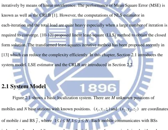
Figure 2.1 shows a basic localization system. There are M unknown positions of

mobiles and N base stations with known positions. ( , , )x y z_{i i i} and (x y z_j, _j, _j) are coordinates

of mobile i and BS j , where 1 i M,1 j N. Each mobile communicates with BSs

independently and mobiles can exchange the information from received signal with each others. In this Chapter, we only concern measurements between mobiles and BSs, cooperative localization will be introduced in next Chapter.

5

Figure 2.1 A basic localization system

In TOA scenario, measured distance d from mobiles to BSs can be calculated by multiplying the propagation time and the signal propagation speed. With TOA measurement from mobile i and BS j, we have measured distance modeled as

,

1, 2,..,

i j i j i j

d



A



n

j



N

(2.1)

where

A

_{i j} is real distance between mobile i and BS j and 2

~ (0, )

i j i j

n N  is modeled as

additive white Gaussian noise (AWGN). We further denote A as a distance function as follow

( )i i , 1, 2,...

i j j

A    BS j N (2.2)

where _i 



x_i y_i z_i



T is the unknown coordinate vector of mobile i and

T

j j j j

BS  x y z _ is the coordinate vector of BS j. From Figure 2.1, we focus on the

position of mobile i, we can rewrite (2.1) in vector term by N measurement data as follow

( )

i i i i

6 where 1 1 1 2 2 2 , ( ) , i i i i i i i i i i iN iN iN d A n d A n d A n d A n                                        

are the measurement vector, distance vector, and

measurement error vector.

We want to utilize these measurements to estimate the position of mobile i. In Section 2.2, some typical LS estimators are introduced.

2.2 Least-Squares Algorithm

According to the model, the unknown position coordinate vector _i can be estimate

based on least-squares theory by searching the minimum of the objective function,





2 2 1

1

ˆ

_min

i N i i j i j j _{i j}

d

BS





















_





_











(2.4)

(2.4) is an optimal solution of LS estimator. It can be written as vector form as 2

ˆ

_{arg min}

_{( )}

i i i _

d

i

A

i _W









(2.5) where ( ) ( ) i T i

W  W denotes a weighted norm with the weight matrix Wi which is

chosen as the inverse of the measurement variance matrix, i.e.,





1 T

i i i

W  E n n_ _  , where W_i

is a diagonal matrix with ₍ 2_{) ,}1 _{1 ~}

i j j N

  _

at j-th diagonal element. With the assumption of normally distributed of measurement errors, the Weighted Least-Squares estimator (WLS) [16] is identical to the Maximum Likelihood Estimator (MLE) [17]. In this thesis, weighting

coefficient will be considered and revised in next chapter.

(2.5) is a nonlinear problem since A involves the norm term, it can be solved by iterative algorithm like the Steepest Descent method, the Newton method, the

7

successfully converge. Our research bases on GN method. Section 2.1.1 introduces the GN method. In Section 2.2.2, some lineared LS methods are given. TLS framework which

reduces the unknown parameter will be introduced in Section 2.2.3. TOA-based CRLB will be given in Section2.2.4.

2.2.1 Gauss-Newton Method

The basic idea of GN method is to linearize the signal model. From (2.2), the non-linear function A_{i j}( )_i can be linearized using Taylor series expansion





,0 ,0 ,

( )_i ( _i ) _{i i} , 1, 2,...

i j i j i j ts i j

A



 A



J

 

 n j  N (2.6)

where n_{ts i j,} is the higher order truncation error of Taylor expansion, and the gradient vector

,0 ,0 ,0 ,0 , , , ,0 ( ) , 1, 2,... T i j i j i j i j i j i j i j i j i j BS x x y y z z J j N A A A BS              _ _ . Then (2.3) becomes ,0 ,0 ,

(

)

(

)

i i i i i i uncoop i

d



A





J

 





n

(2.7)

where _i,0 is the initial vector and

n

uncoop i,



n

ts i,



n

i denotes the total error including

higher order truncation error of Taylor expansion and measurement noise, where

, 1 , 2 , , T ts i ts i ts i ts iN n n n n                . Ji RN 3 

 (3 dimensions) is uncooperative Jacobian matrix [18],

,0 1 ,0 1 ,0 1 1 1 1 1 ,0 2 ,0 2 ,0 2 2 2 2 2 ,0 N ,0 N ,0 N N N N i i i i i i i i i i i i i i i iN i i i i i i x x y y z z A A A J x x y y z z J A A A J J x x y y z z A A A           _{  }     _{  }    _{  }  _{  }  _{  }  _{     }     (2.8)

8

According to (2.7), the estimate location of the mobile i (2.5) can be written as 2 ,0 ,0 ˆ _{arg min ( ) ( )} uncoop i i _ di Ai i Ji i i _W



 





 

 (2.9)

the GN method solves the problem by iteratively minimizing the new objective function, 1 , 1 , , , , , , , , , ˆ ˆ ₍ T ₎ T _{( (}ˆ ₎₎ i k i k Ji k Wuncoop i kJi k Ji k Wuncoop i k di Ai i k









    (2.10)

where the weighting matrix is covariance inverse of

n

_{uncoop i,} ,





1

, , , , , ,

T uncoop i k uncoop i k uncoop i k

W  E n_ n _  (2.11)

The element of Wuncoop i k, , is a diagonal matrix with

2 2

, , , , , , , 1 ~

T

uncoop i k uncoop i k _{j j} ts i j k i j

E n_ n  _   j N (2.12)

In (2.10), there exists 3 3 matrix inverse with highly computational cost. Note that we can

omit the Taylor truncation error if there is a good reference point. In (2.10), Ji k, , Ai(



i k, )

can affect the position accuracy and will be updated with the k-th i k, . The GN method

explores the quadratic form of the objective function and is adequate for solving

(small-residual) non-linear problem, but the complexity is cumbersome. In next Section, three linearization algorithms will be introduced to reduce its computational cost.

2.2.2 Linearization of Least-Squares Method

There are three common linearization methods, Taylor-series expansion algorithm (TS) [10], distance-augmented algorithm (DA) [11] and hyperbolic-canceled algorithm [12]. We summarize them as follows. By linearizing the non-linear term, (2.2) can be written as

i L

bH



n (2.13)

the terms b H, of three linearization methods had been derived in the literature. Applying

9 1

ˆ

₍

T

₎

T i

H W H

L

H W b

L



_

 (2.14)

where W is the weighted matrix. The covariance matrix of _L

e

_i

 

 

ˆ

_{i i} is





1

cov( )e_i  H W HT _L  (2.15) and the Mean-Square-Error (MSE) of the estimator is

(cov( ))i

MSEtrace e (2.16)

The LLS estimators are easy to operate and cost less computation compared with iterative methods. It is trade-off between cost and accuracy. Some researches try to reduce the complexity with high accuracy. [19] utilize constrained least-squares method. [20] uses one range measurement in each iteration to update the user position. We introduce transformed least-squares (TLS) framework [13] which reduced the parameter of unknown parameters in Section 2.2.3.

2.2.3 Transformed Least-Squares Framework

Instead of the traditional LS estimator, Transformed Least-Squares (TLS) [13] tries to keep the required computations low in two steps. The first step is transforming the positioning problem to lower dimensions. There are three dimensions (3-D) in original 3-D localization problem. Once the dimensions are less, the unknown parameters to be estimated are less respectively. Second, solve the remaining parameters iteratively. [13] proposed a one

dimensional iterative (1DI) method that the LLS method is used to transform the problem to one dimension and an iterative method is used to estimate the 1-D unknown parameter. Actually, the idea of TLS can be explained as follow. In classical nonlinear LS (NLS) algorithm (2.4), the unknowns are estimated together. On the other hand, it can be divided to

one unknown (z ) nonlinear problem and other two dimension ( ,_i x y ) nonlinear estimation. _{i i}

10 i

z , the estimation problem become one dimension, i.e.,

, , ,

ˆ _{min ( , , ) min min ( , , ) min ( ( ), ( ), )}

i i i i i i i

i i i i i i i i i i i i

x y z f x y z z x y f x y z z f x z y z z

    (2.17)

f denotes objective function in (2.4). From (2.17), [13] divides the original three dimensions

nonlinear problem to one dimension since the x-axis and y-axis coordinate of mobile i is

transferred to linear function of z . The reduced-dimension localization problem can be _i

solved based on the GN method introduced in Section 2.2.1. In [13], the mapping function is given based on hyperbolic-canceled algorithm mentioned in Section 2.2.2,



ˆ ˆ



( 2 ) T i i i x y m b H z (2.18) where 2 2 , 1 ~ , T T j j N i i N N b d d BS BS BS BS j N m(H W H_{1 L 1})1H W_1L ,





1 2 1 1 1 1 2 1 1 1 2 N N N N N N N N N H H x x y y z x H H H x _ x y _ y z _ z    _{  }          _{  }        .

The mapping in (2.18) is fixed by mapping coefficients H₁, H₂ and b. Based on (2.18), the

position of mobile i can be written as





T i xi yi zi f Fzi     (2.19) where , 0 mb f       2 , 1 mH F  _   3 ,

f FR . Then, (2.5) can be written as

2

ˆ

arg min

(

)

i i i i i _W z

z



d



A f



Fz

(2.20)

Finally, the problem has transformed to one dimension nonlinear Least-Square problem

according to the variable

z

_i, which can be solved by GN method iteratively. The TLS method

not only reduces the computations but preserves performance comparable with GN method. In cooperative localization, the dimensions of unknowns are quite high by the positions of

11

mobiles. We propose a dimension reduced Least-Squares algorithms based on TLS framework, and the additional challenge from measurements between mobiles are another issue which will be described in Chapter 3.

2.2.4 Cramer-Rao Lower Bound

In previous section, mobile i can be estimated through uncooperative measurements. For comparison with these estimators, the CRLB is given as a criterion. Based on [22], the error covariance matrix of position error vector

e

ˆ

_i

 

 

ˆ

_{i i} satisfies Information Inequality

1 ˆ ˆ ˆ cov( ) i T i i i e E e e_ _I_ (2.21) where 1 i

I

_ is the full uncooperative Fisher Information Matrix (FIM) for mobile i

2 2 2 2 2 2 2 2 2 2 2 2 2 ( ) ( )( ) ( )( ) ( )( ) ( ) ( )( ) 1 ( )( ) ( )( ) ( ) i i j i j i j i j i j i j i j i j i j i j i j i j i j i j i j i j i j i j i j i j i j i j i j i j i j x x x x y y x x z z A A A x x y y y y y y z z I A A A x x z z y y z z z z A A A  _             _{    }     _{ }    _{    }        1 N j



(2.22)

Then, the trace of inverse of 1

i

I

_ in (2.21) is defined as the lower bound for MSE, Therefore,

uncooperative CRLB is given by

1

i

uncoop

CRLB   tr I _  (2.23)

12

Chapter 3

Cooperative Localization System

Cooperative localization is raising up as a new branch of wireless localization in which several researches are being explored. By the development of short-range communication such as UWB, the direct communication of different terminals can be used in cooperative positioning. [17] considers that the short-range measurements are reliable to enhance the accuracy of location and investigate the data fusion of large-scale and small-scale.

In cooperative system, the distance measurements between any pairs of unknown positions mobiles are utilized to improve the location estimation. To mobile i, the

measurement distances between BSs and the other mobiles are combined as the information of which are used to solve the estimation problem. The other unknown mobiles play a role as virtual BSs to assist mobile i in localization. In cooperative localization, the location accuracy of virtual BS is important since the un-precise virtual BS may cause the degradation of

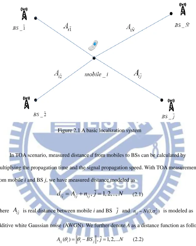
localization. It is a more critical task than conventional localization due to the additional information from mobiles to mobiles. Figure 3.1 indicates the cooperative localization system. There are N known positions of BSs and M unknown positions of mobiles. Our purpose is to

estimate all the M unknown positions of mobiles by using total (M N C M( , 2))

measurement data. From figure 3.1, mobile i receives N TOA measurement from known

positions of BS and (M-1) measurements from unknown positions of mobile. A_{i j} is the real

distance between mobile i and BS j which is mentioned in section 2.1; the cooperative term

ij

13

Figure 3.1 Cooperative localization system

The cooperative measurement between mobile i and mobile j is denoted as

, , 1, 2,.., 1 , , 1,..,

ij ij ij

d  A n i j i M  ji i M (3.1)

where

n

_ij

~

N

(0,



_ij2

)

is cooperative measurement error modeled as AWGN. Combining (2.1)

and (3.1), the cooperative measurement model can be writtene as

( )

d



A





n

(3.2) where _{1 2} T T T T M

_{ }   _ is the position vector of M mobile and

1 1 1 ( ,2) 12 12 12 1, 1, 1, , ( ) , ; , , T T T N N N M N C M M M M M M M d A n d A n d A n d A n R d A n d A n                                                                    . Further denote ! ( , 2) ( 2)!2! M C M M

 _{ . The M unknown position coordinates can be estimated}

14





2





2 2 2 1 1 1 2 1 1 ˆ min arg min ( ) M N M i ij i j i j j i j i j i ij j i Noncooperation cooperation W d BS d d A  





 







           _      _        





(3.3).

Compared with (2.4), (3.3) takes additional information in account and we can see that cooperative localization is a tough issue than uncooperative localization. On the other hand, the reliability of additional cooperative measurements is another issue; if the unreliable

measurements are used (_ij2 is large), the localization accuracy becomes worse. Simulation

shows the influence on noise variance in Section 4.2.1.

There are several ways that can be used to solve LS estimator (3.3). Nonlinear iterative algorithms estimate the location with high performance, but the complexity is quite high. By linearized algorithm, the costs can be reduced, but the performance is sacrificed. Here, we propose three pre-linear methods with low complexity but good accuracy. The structure of the rest of this section is as follows. Section 3.1 discusses cooperative GN method. The pre-linear method of auxiliary mobiles is proposed in Section 3.2. Section 3.3 derives the

dimension-reduced GN algorithm for target mobile. Weighting compensation and mobile selection are discussed in Section 3.4 and Section 3.5 respectively. In the end, the

computation is compared in Section3.6.

3.1 Cooperative Gauss-Newton Method

In cooperative localization, GN method is also useful to solve (3.3). According to

Section 2.2.1, the additional cooperative term is discussed. Section 3.1.1 derives joint GN method. Divided GN method is given in Section3.1.2.

15

3.1.1 Joint GN Method

We know that unknown positions of mobiles are involved in cooperative system. In

addition to (2.1), the remaining task is to linearize cooperative nonlinear distance function

( , )

ij i j i j

A

 



 

 (3.4)

Apply Taylor-series expansion to (3.4) with initial value

 

i,0

,

j,0 as follows

,0 ,0 ,0 ,0 , , ( , ) ( , ) ( , ) i j T ij i j ij i j ij i j ts ij A A A n                  

where

n

ts ij, is the higher order truncation error of the Taylor-series expansion for

A

ij

,

,0 ,0 ,0 ,0 ,0 ,0 , ( , ) ( , ) ( , ) i j i j T ij i j ij i j T T ij i j ij ij A A A h h               _{ }  _{ }  _  _   _ ,

and

h

ij is the cooperative gradient vector between mobile i and mobile j.



,0 ,0



,0 ,0 ,0 ,0 , i j i i ij j j i j h              _{   }   _{ } (3.5)

Now the cooperative measurement model (3.1) becomes

,0 ,0 ,

( , ) T T

ij ij i j ij ij coop ij

d A

 

_h h _ n (3.6)

where

n

_{coop ij,}



n

_{ts ij,}



n

_ij denotes total cooperative error including Taylor truncation error and cooperative measurement error. (3.6) is a linear equation of cooperative measurement model. Collecting all the uncooperative linear equation (2.6) and cooperative linear equation (3.6) with M=4, joint GN Jacobian matrix equation is given by

0 0

( )

(

)

16 where 1 2 3 4 12 12 13 13 14 14 23 23 24 24 34 34 0 0 0 0 0 0 0 0 0 0 0 0 0 0 0 0 0 0 0 0 0 0 0 0 T T T T T T T T T T T T J J J J h h J h h h h h h h h h h              _         _        _         , 1 ,1 2 ,2 3 ,3 4 ,4 12 ,12 13 ,13 14 ,14 23 ,23 24 ,24 34 ,34 ts ts ts ts uncoop ts coop ts ts ts ts ts n n n n n n n n n n n n n n n n n n n n n n n     _        _     _       _{ }       _        _         (3.8)

J is cooperative Jacobian matrix. The term uncooperative Jacobian matrix J_i is same as

(2.8), , ( 0), ( ,2)

M N C M

d A



R   are the measurement data, distance function which contained

both uncooperative and cooperative term. Further denotes

n

is the total error vector

including Taylor high order truncation error and noise. According to (3.7), the objective function is denoted as 2 0 0 ˆ arg min ( ) ( ) W d A J 



 





 

 (3.9)

and the joint GN estimator solves (3.9) iteratively by 1 1

ˆ

ˆ

₍

T

₎

T

₍

_{( ))}

ˆ

k k

J W J

k k k

J W d

k k

A

k











 



(3.10) , 1 , 0 ( ) 0 uncoop k T k k k coop k W W E n n W       _{    }  

Here,

J

k denotes kth cooperative Jacobian matrix which is different from

J

i in (2.8).

and W_{coop k,} is covariance inverse of

n

coop k, ,





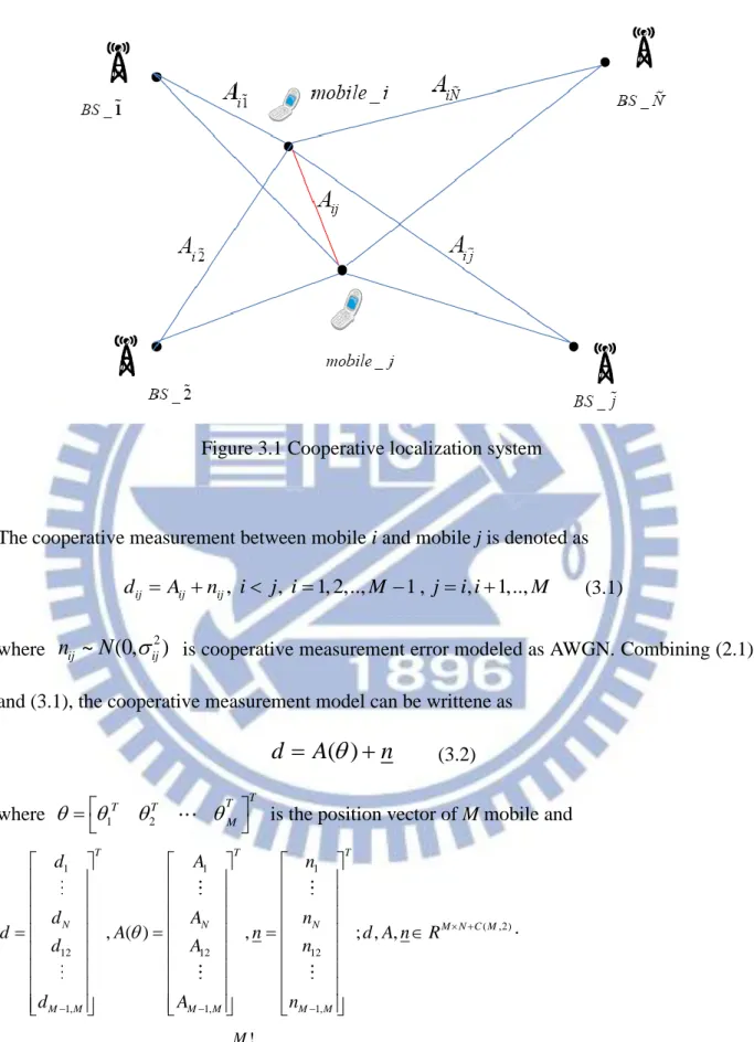
1

, , ,

T coop k coop k coop k

W E n n



 

 _{ }

17 12 2 2 ,12, , , 2 2 ,12, ( 1) 0 0 ts k T coop k coop k ts k M M E n n     _       _{   }    _    k

W is a diagonal matrix which including

W

uncoop k, in (2.12) and cooperative term. Note that

there is 3M3M inverse matrix 1

( T )

k k k

J W J  in (3.10) which includes highly computational

cost. Besides, we can omit the Taylor truncation error as before if there is a good reference point. In Section 4.4.1, the effect on Taylor truncation error from initial value will be shown. In (3.10), the positions of mobiles are updated jointly with high position accuracy. In section 3.1.2, the divided method which updates the position of mobile individually will be described.

3.1.2 Divided GN Method

We know that if there exists a mobile j with known position, it can be regarded as a virtual BS to mobile i and can be helpful to estimate mobile i. Figure 3.2 illustrates the above description.

Figure 3.2 Cooperative localization with virtual BS _j

18

From Figure 3.2, the position of every single mobile can be estimated by measurements from

true BSs and other virtual BSs. To mobile i, the LS searches a



ˆ

_i which minimizes the

objective function





2





2 2 2 1 1, 1 1 ˆ _{min , 1, 2,..,} i N M i i i j ij i j j i j j j i ij cooperation noncooperation d BS d i M 





 





          _      _       





(3.11)

where



_j denotes known position of virtual BS. Note that (3.11) only include the unknown

parameter of mobile i. However, the uncertain positions of virtual BSs may degrade the accuracy. To deal with this problem, the individual uncooperative localization (2.4) is used to find a not-bad initial value of virtual BS. Then, (3.11) estimates the positions of mobile i.

1 , , ˆ ₍ T ₎ T i H W Hi L i i H W bi L i i



_  (3.12)

Every individual mobile can be updated by other M-1 virtual BSs iteratively to improve the position accuracy. Actually, Jacobi and Gauss-Seidel methods [18] are used to choose the positions of virtual BSs. Our proposed parallel and sequential pre-linear methods are based on Jacobi and Gauss-Seidel methods, respectively. Figure 4.6 shows the comparison between divided method and pre-linear methods. The divided method can reduce the computation costs most in (3.10), but the performance is sacrificed.

3.1.3 Cooperative CRLB

In cooperative system, cooperative CRLB is given as uncooperative system that is to be

a standard to estimators in this Chapter. The full cooperative Fisher Information Matrix can be written as follows

19 1 2 1 12 1 1 1 12 2 2 1 2 1 2 1 M M i M i i M i M i i M M M Mi i i M I I I I            _{  }         _{  }                     







C C C C C C C C C (3.13) where i

I_ is the uncooperative FIM in (2.21) for mobile i and C_ij is cooperative

information matrix between mobile i and mobile j which is denoted as

2 2 2 2 2 2 2 2 2 2 2 2 2 ( ) ( )( ) ( )( ) ( )( ) ( ) ( )( ) 1 ( )( ) ( )( ) ( ) i j i j i j i j i j ij ij ij i j i j i j i j i j ij ij ij ij ij i j i j i j i j i j ij ij ij x x x x y y x x z z A A A x x y y y y y y z z A A A x x z z y y z z z z A A A              _{    }                    C (3.14)

Then, the cooperative CRLB for mobile i is

1 coop

CRLB   tr I   (3.15)

Note that the cooperative CRLB for mobile 1 lies at the upper-left block

1

1 , upper-left 3 3submatrix of coop mobile

CRLB tr_  I_ _

Simulation compares our methods with (3.15) in Section 4.1. In Section 3.2, we propose a low complexity with high accuracy pre-linear methods in cooperative localization.

3.2 Pre-Linear Methods of Auxiliary Mobiles

In cooperative system, the M mobiles positioning problem is presented. In Section 3.1, joint GN method outperforms divided method, but the total costs are higher than divided method. Instead of GN method, we try to seek a relation between mobiles by re-formulating the positioning problem to reduce the number of unknown mobiles based on [13]. In this way, we expect that the proposed pre-linear methods have good performance in both accuracy and

20

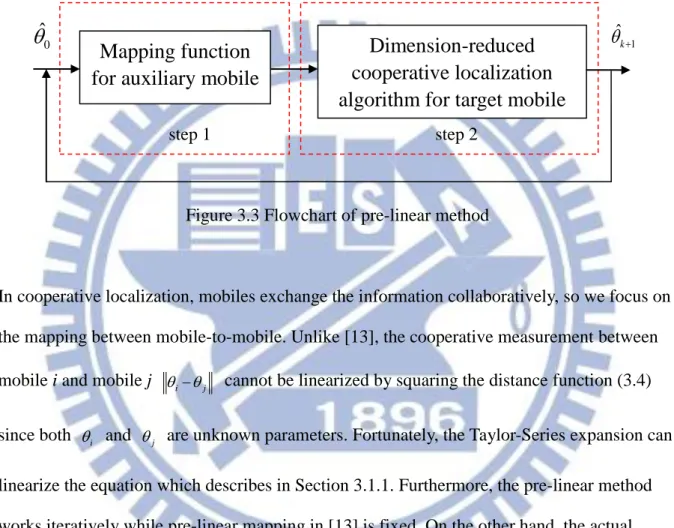
complexity. The basic idea of pre-linear method consists of two steps: The unknown of parameters are reduced in step 1 by pre-linear mapping, and the localization algorithm for remaining unknown parameters in step 2 using the pre-linear function in step 1. Figure 3.3 indicates the flowchart of the pre-linear method. In Figure 3.3, we aim at searching a mapping function between unknown positions of mobiles.

step 1 step 2

Figure 3.3 Flowchart of pre-linear method

In cooperative localization, mobiles exchange the information collaboratively, so we focus on the mapping between mobile-to-mobile. Unlike [13], the cooperative measurement between

mobile i and mobile j  _i _j cannot be linearized by squaring the distance function (3.4)

since both _i and _j are unknown parameters. Fortunately, the Taylor-Series expansion can

linearize the equation which describes in Section 3.1.1. Furthermore, the pre-linear method works iteratively while pre-linear mapping in [13] is fixed. On the other hand, the actual mapping relations between mobiles are not existence, we can also correct the mapping by iteration.

Once the pre-linear mapping is obtained, the dimension of unknown parameters to be estimated can be reduced, and the localization algorithm is simplified accordingly. However, there is a lot of combination of mapping relation, the choice of mapping function is based on different localization requirement. Our purpose is to simplify the algorithm in (3.10), so the linear mapping is a suitable choice which reduces the complexity most. The following

1

ˆ

k  _

Mapping function

for auxiliary mobile

Dimension-reduced

cooperative localization

algorithm for target mobile

0

ˆ

21

describes the two steps of the pre-linear method.

In Step 1, we select a mobile called “Target” mobile which is chosen as a reference mobile to be estimated in step 2; and the others called “Auxiliary” mobiles that are restricted to be a linear function of the target mobile. It is assumed that there exists some linear mapping relation between auxiliary mobile and target mobile. Without loss of generality, we select

mobile 1 as a target mobile, and mobile 2 ~M as auxiliary mobiles, i.e.,



q



L

q

( )



1 , q

=2,3,…,M. Therefore, (3.2) can be rewritten as



1

,

1

( ),

1 2

( ),..,

1 M

( )

1



d



A



L



L



L





n

(3.16)

By linear mapping function L, the auxiliary mobiles can be transformed to the linear function of the target mobile. However, mobiles are located at different positions independently so an error-free mapping is usually not available. How to find a proper mapping function by measurement data becomes a critical issue. We propose three linearized mapping methods to implement the mapping function. The detail will be described in the next section.

In Step 2, once the mapping function is generated, LS estimator can solve the dimension-reduced cooperative localization problem based on (3.16).

1 2 1 1 1 1 2 1 1

ˆ

_{arg min}

_{( ,}

_{( ),}

_{( ),..,}

_{( ))}

M _W

d

A

L

L

L

















(3.17)

We only consider the parameters of target mobile in this step unlike the original multiple mobiles in (3.3). In section 3.3, Dimension-reduced GN method is derived based on the GN

algorithm mentioned at section 3.1. The original 3M3M (3-D case) inverse matrix

problem in (3.10) can be transferred to 3 3 positioning problem. Therefore, the computation

cost is reduced efficiently. The detail of computation costs will be described in Section 3.6. We note that if the position of target mobile is updated, the corresponding positions of auxiliary mobiles can be obtained by using mapping function and the position of target mobile we estimated. Figure 3.4 indicates the description above.

22

Target mobile auxiliary mobiles Figure 3.4 The diagram of mapping from target mobile to auxiliary mobiles

In Figure 3.4, the accuracy of target mobile affects the accuracy of auxiliary mobiles by the

mapping functionL( )₁ . The reliable target mobile can improve the accuracy of auxiliary

mobiles. In Section 3.5, we propose a target mobile selection method to find the reliable target mobile. In fact, the auxiliary mobiles are used cooperatively to search the mapping function which is inserted in the cost function in step 2 (see (3.17)), so auxiliary mobiles and target mobile interact with each other. The uncertain position of mobiles may deteriorate the

localization accuracy. Therefore, the compensation of weighting coefficient will be derived in Section 3.4.

3.2.1 Joint Pre-Linear Method

There are M unknown positions of mobile in localization system. Our purpose is to find the relation between these M positions of mobile which is described in previous section.

In joint pre-linear method, we want to find a mapping function so that all the (M-1) auxiliary mobiles can be written as a function of target mobile jointly. i.e.,

2 3 ( )1 T T T T M L          (3.18)

where L is a linear mapping from R3R3(M1). Figure 3.5 depicts the mapping relation of

joint pre-linear method. 1



2( )1 L  3( )1 L  LM( )₁ 1

( )

L



23

…

_{target mobile}

Auxiliary mobiles

Figure 3.5 Mapping relation of joint pre-linear method

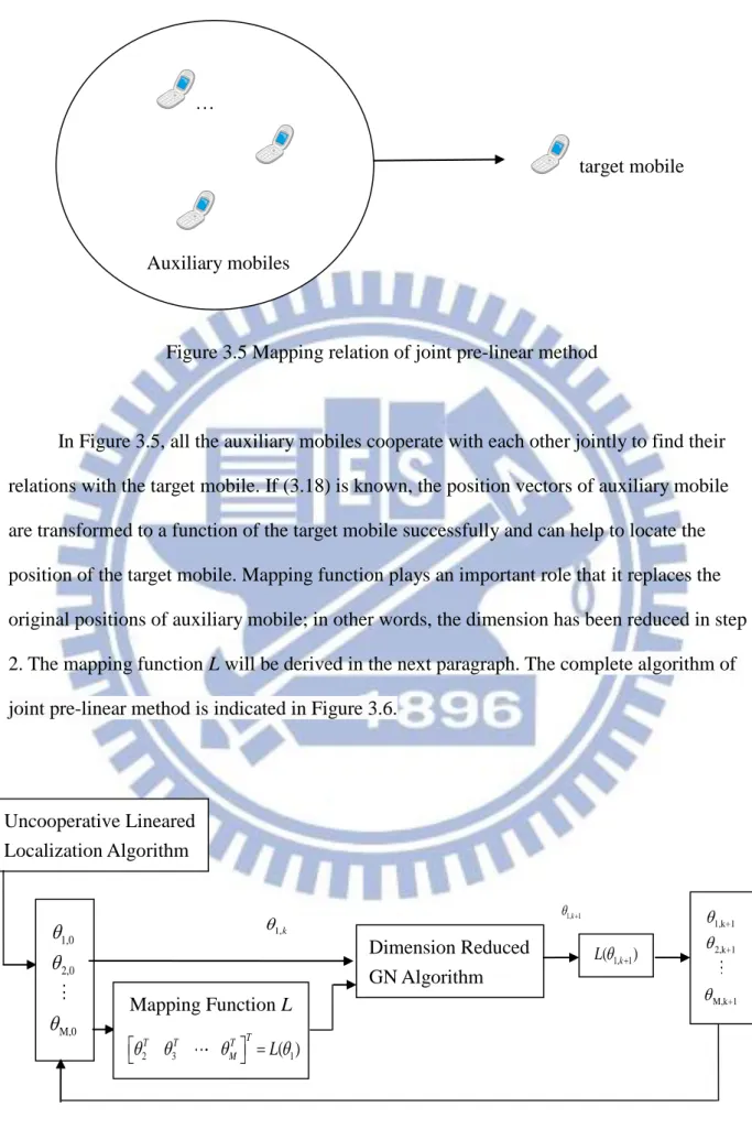
In Figure 3.5, all the auxiliary mobiles cooperate with each other jointly to find their relations with the target mobile. If (3.18) is known, the position vectors of auxiliary mobile are transformed to a function of the target mobile successfully and can help to locate the position of the target mobile. Mapping function plays an important role that it replaces the original positions of auxiliary mobile; in other words, the dimension has been reduced in step 2. The mapping function L will be derived in the next paragraph. The complete algorithm of joint pre-linear method is indicated in Figure 3.6.

Figure 3.6 Joint pre-linear algorithm Uncooperative Lineared Localization Algorithm 1,0 2,0 M,0    Mapping Function L 2 3 ( )1 T T T T M L          Dimension Reduced GN Algorithm 1, 1 ( k ) L  1,k+1 2,k+1 M,k+1    1,k  1, 1k

24

Fortunately, we can get the mapping function by linearizing the cooperative nonlinear function (3.2) using Taylor-series expansion. Rearranging (3.7) with M mobiles and the linear equation is given

y



J





n

(3.19)

where J is cooperative Jacobian matrix which is same as (3.7),

( ,2) 0

;

,

uncoop _{M N C M} uncoop coop coop

y

y

d

J

y

R

y

R

y











_

_

 













We further denote

F

_i as the i column of J, and (3.19) can be rewritten as





1 2 1 2 M M

y

F

F

F

n



































(3.20)

Note that ₁ is the position vector of the target mobile. From (3.20), we can see that if we

regard ₁ as a variable parameter of equation and shift the term

F

_{1 1}



to the left-hand side

of the equation as follows,





2 3 1 1 2 3 M M y F F F F n









               (3.21)

the position vector of target mobile



₁ is used to solve the linear equation (3.21) with

unknowns '



2 3



T M











. Note that the dimension in (3.20) is 3M but 3(M-1) in

(3.21). According to (3.21), in the k-th iteration, the linear LS estimator mentioned in Section 2.1.2 can solve the problem as follow

' ' ' 1 ' 1, 1,

(

T

)

T

(

)

k

F W F

k k k

F W y

k k k

F

k k



_



_



(3.22)

25

We denote auxiliary Jacobian matrix Fk'  F2,k F3,k FM k, , taget Jacobian matrix

1,k

F , and weighting matrix is same as (3.10). The linear mapping function is generated

successfully in (3.22). The terms F , k' F , and 1,k yk include information of unknown

parameter which are updated by the (k-1)-th solution shown in figure 3.6, we can understand

that the mapping function is updated iteratively. We should note that



k' is not the k-th

iteration solution of auxiliary mobile since (3.22) is the function of variable _1,k. The

solution will be updated after the algorithm in step 2. In addition, (3.22) can be simplified as

' int, int. 1 k

g

jo k

G

jo k k









(3.23) where ' ' 1 ' 3( 1) int,

(

)

T T M jo k k k k k k k

g



F W F



F W y



R

 ' ' 1 ' 3( 1) 3 int,

(

)

1, T T M jo k k k k k k k

G

 

F W F



F W F



R

  (3.24)

The mapping coefficients

g

joint and Gjoint will be updated and become more accurate by

iteration. We can obtain the linear mapping between every single auxiliary mobile and target mobile by separating (3.23),

'

int, , int, , 1,

;

2,3,..,

k

g

jo i k

G

jo i k k

i

M











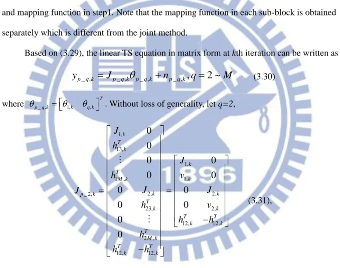
(3.25)

In (3.25), we can see that the position vector of auxiliary mobiles becomes a linear function of position vector of target mobile. The linear mapping equation is generated by revising linear LS formulation. Here, we give a example if number of mobiles is equal to 4. The cooperative linear model in case M=4 can be written as

26 1, 1, 2, 2,k 3, 3,k 4, 4,k 12, 12, 12, 13, 13, 13, 14, 14, 14, 23, 23, 23, 24, 24, 24, 34, 34, 34, 0 0 0 0 0 0 0 0 0 0 0 0 0 0 0 0 0 0 0 0 0 0 0 0 k k k k k T T k k k T T k k k T T k k k T T k k k T T k k k T k k k y J y J y J y J y h h y h h y h h y h h y h h y h h               _         _        _        ,1, 1 ,2, 2 ,3, 3 1, ,4, 4 2, ,12, 12 3, ,13, 13 4, ,14, 14 ,23, 23 ,24, 24 ,34, 34 ts k ts k ts k k ts k k ts k k ts k k ts k ts k ts k T ts k n n n n n n n n n n n n n n n n n n n n             _            _{ }  _   _{ }    _{ }  _   _{ }    _{ }    _{ }  _           _                  (3.26) where , ( , ) ( , ) , i k i i k i i k i k r A  J   , , ( , , , ) , , , , ij k i j i k j k ij k i k ij k j k r A   h  h  , , , i k i i k i k

y

 

d

r r

y

ij k,



d

ij



r

ij k, _(3.27)

Note that the Taylor higher order truncation error can be omitted if the reference point is good enough. Here, there are 4N pairs of measurements between mobiles to BSs and C(M,2)=6 pairs of cooperative measurement between mobiles. Based on (3.22), the mapping function can be written as ' ' 1 ' 2, 3, 4, ( ) ( , 1, 1, ) T _{T T} k k k F W Fk k k F W yk k l k Fk k            (3.28) where ' 2, 3, 4, k k k k

F  F F F _. We can see that the row 1~N are zeros in

F

_k, and the mapping

function is similar to the divided method which regards



1,k as a virtual BS with known

position to other M-1 mobiles. On the contrary,



1,k in (3.28) is still a variable parameter

that will be updated in the next step; F_1,k_1,k is the revised term which adjust the cooperative measurement between target mobile and other 3 auxiliary mobile by gradient vector between

27

target mobile and auxiliary mobile j h1j, j2 ~ 4, and the first element J1,k in F1,k is

useless since J_1,k is the term that related to the uncooperative measurement between target

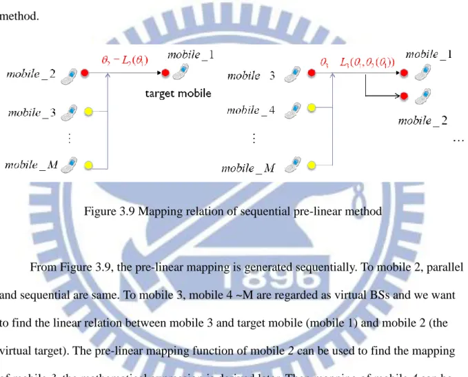
mobile and BSs. The detail of mathematical expression for (3.28) will be given in Section 3.6. With the linear mapping function, the original model can be changed to one unknown mobile problem; it is same as the following two pre-linear method. In Section 3.3, the

dimension-reduced GN algorithm will be derived.

3.2.2 Parallel Pre-Linear Method

We have derived the joint pre-linear method in the previous Section. In (3.22), there

still remains 3(M  1) 3(M 1) matrix inversion even though it is better than 3M3M

matrix inversion in original GN algorithm. Based on section 3.1.2, we can further reduce the complexity of the mapping function.

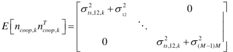
Instead of joint method, we can derive the mapping function individually in parallel pre-linear method based on Jacobi method [18]. The following figure depicts the mapping relation of parallel pre-linear method.

Figure 3.7 Mapping relation of parallel pre-linear method

We illustrate the parallel method for mobile 2 and mobile 3 in Figure 3.7. Auxiliary mobiles find the relation with target mobile individually. To auxiliary mobile q, it regards the

28

other (M-2) auxiliary mobile as virtual BSs; the localization scenario becomes N fixed BSs and (M-2) virtual BSs with two unknown positions of mobiles that contained one target and one auxiliary mobile. To every individual mobile in Jacobi method, other (M-1) are regarded as virtual BS with known position. In pre-linear methods, the position of target mobile is still unknown which is different from divided method, we find the linear mapping between

auxiliary mobiles and target mobile and utilize the pre-linear function to estimate the position of target mobile. The LS estimator for mobile 1 (target mobile) and mobile q (auxiliary mobile) is given by

















1, 2 2 1 1 1 1 2 2 1 1 2 1 1 virtual BSs 2 2 q q 2 2 1 q 2 q 1 1 ˆ min ˆ q _{1 1} N M j j j j j j j j j q Noncooperation N q q j q j j j j j j j j Noncooperation d BS d d BS d          _{  }                           











2 1 1 2 1 virtual BSs 1 ; 2 ~ q q M q cooperation q d   q M               _{   }  _                 _{ }   



(3.29)

where _j denotes known position virtual BS. The complete algorithm of parallel pre-linear

method is indicated in figure 3.8.

Uncooperative Lineared Localization Algorithm 2 L( 1)    3, 4,.., M    Dimension Reduced GN Algorithm 1, 1 ( k ) L  1,k+1 2,k+1 M,k+1    1,k  1, 1k 3 L( 1)    2, 4,.., M    1 ( ) M L    3, 4,.., M1     1,0 2,0 M,0   