利用位元壓縮法的快速封包分類演算法

全文

(1)國立交通大學資訊科學系碩士論文. 利用位元壓縮法的快速封包分類演算法 Fast Packet Classification Using Bit Compression. 研究生：許嘉仁指導教授：陳. 健. 博士. 中華民國九十三. 年六月.

(2) 利用位元壓縮法的快速封包分類演算法 Fast Packet Classification Using Bit Compression. 研究生：許嘉仁. Student：Chia-Ren Hsu. 指導教授：陳. Advisor：Chien Chen. 健. 國立交通大學資訊科學研究所碩士論文. A Thesis Submitted to Institute of Computer and Information Science College of Electrical Engineering and Computer Science National Chiao Tung University in partial Fulfillment of the Requirements for the Degree of Master in Computer and Information Science June 2004 Hsinchu, Taiwan, Republic of China. 中華民國九十三年六月.

(3) 利用位元壓縮法的快速封包分類演算法研究生：許嘉仁. 指導教授：陳健博士. 國立交通大學資訊科學研究所. 摘要為了提供安全防護，虛擬私有網路，品質保證等等網際網路的服務。網際網路路由器需要將收到的封包進行快速的分類。封包分類是利用在封包標頭所包含的資訊與路由器中事先定義的規則表進行比對，一般而言，多重欄位的封包分類是一個相當困難的問題，已經有許多不同的演算法被提出來解決這個問題。在這篇論文中，我們提出一個稱為位元壓縮(bit compression)的封包分類演算法。如同眾所周知的位元圖交集(bitmap intersection)演算法，位元壓縮也採用多維區域查詢 (multiple dimensional range lookup)的方法。觀察位元圖交集演算法中的位元向量 (bit vector)，我們發現在位元向量中包含許多的 0 位元，利用這個特性，我們將位元向量進行壓縮，藉由保留有用的資訊，建立一個用來記錄剩餘位元相對應的規則號碼之索引表，以及移除位於位元向量中多餘的位元來達成壓縮的目的。此外，利用有百搭符號的規則(wildcarded rule)可以更進一步地提高壓縮的比例。透過實驗結果的觀察，位元壓縮演算法可以將儲存空間的複雜度由位元圖交集演算法的O(dN 2)減低為O(dN·logN)，而不犧牲封包分類的效能，在這裡d表示維度的個數，而N表示規則的個數。在封包分類的效能上。因為位元壓縮演算法只需要比位元圖交集演算法更少的記憶體存取時間，而在封包分類的問題中，記憶體的存取往往決定了整體的查詢時間，所以，即使位元壓縮需要額外的解壓縮的步驟，仍會有比位元圖交集演算法更快的分類速度。 I.

(4) Fast Packet Classification Using Bit Compression Student: Chia-Ren Hsu. Advisor: Dr. Chien Chen. Department of Computer and Information Science National Chiao Tung University Hsinchu, Taiwan, 300, Republic of China. Abstract In order to support Internet security, virtual private networks, QoS and etc., Internet routers need to classify incoming packets quickly into flows. Packet classification uses information contained in the packet header to look up the predefined rule table in the routers. In general, packet classification on multiple fields is a difficult problem. A variety of algorithms had been proposed. This thesis presents a novel packet classification algorithm, called bit compression algorithm. Like the previously well known algorithm, bitmap intersection, bit compression is based on the multiple dimensional range lookup approach. Since the bit vectors of the bitmap intersection contain lots of ‘0’ bits. Utilizing those ‘0’ bits, the bit vectors could be compressed. We compress the bit vectors by preserving only useful information but removing the redundant bits of the bit vectors. An additional index table would be created to keep tract of the rule number associated with the remaining bits. Additionally, the wildcarded rules also enable more extensive improvement. Our experiment results show that the bit compression algorithm reduces the storage complexity from O( dN 2 ) of the bitmap intersection algorithm to O(dN·logN), where d denotes the number of dimensions and N represents the number of rules, without sacrificing the classification. II.

(5) performance. On the classification performance, the bit compression algorithm requires much less memory access time than bitmap intersection algorithm. Since memory access dominates the lookup time. Even though extra processing time for decompression is required for the bit compression algorithm, the bit compression scheme still outperforms bitmap intersection scheme on the classification speed.. III.

(6) 致謝. 這篇論文的完成，有許多協助與支持我的人需要感謝。首先，最感謝的是我的指導教授，陳健博士，老師總在我有疑問時耐心地給予指導，在我遇到挫折時適時地給與勉勵，在我鬆懈時耳提面命地給予苦口婆心的叮嚀。在研究的路上，自己常常往錯誤的方向嘗試，而老師總是不厭其煩地指引我正確的道路。因為老師無私的付出。讓我得以順利完成這篇論文。此外，在做學問的態度以及待人處事各方面老師亦給我很大的啟發，謝謝老師。其次，要感謝我的口試委員，林盈達博士，李政崑博士以及何慎諾博士，謝謝老師們針對我的研究所提出的寶貴意見，讓我得以對缺失與不足的部分加以改善，豐富了這篇論文的內容與價值。再者，要感謝實驗室裡的各位學長、同學以及學弟們的鼓勵，謝謝吳奕緯學長、葉筱筠、陳盈羽、羅澤羽、官政佑、林俊源、王獻綱、徐勤凱、陳咨翰以及劉上群。謝謝各位陪我度過低潮與不順利的時刻，讓我能有快樂充實的研究生生涯。特別是最後幾個月忙碌的生活，更讓我感受到大家是那麼樣熱情地給予協助，真的是十分難忘。最後，感謝我的家人給予我的栽培與支持，他們的鼓勵一直是我一路走來最大的動力。在此，向我的家人致上我最深的謝意。. IV.

(7) Table of Contents. Abstract (In Chinese)................................................................................................... I Abstract....................................................................................................................... II Acknowledgement (In Chinese)............................................................................... IV Table of Contents........................................................................................................ V List of Figures............................................................................................................ VI List of Tables..............................................................................................................VII. Chapter 1. Introduction.............................................................................................. 1 Chapter 2. Performance Metrics and Related Works............................................. 5 2.1 Performance Metrics for Packet Classification Algorithms............................ 5 2.2 Related Works................................................................................................. 6 Chapter 3. Proposed Bit Compression Algorithm...................................................12 3.1 Using Bit Compression to Reduce Storage Space......................................... 12 3.2 Measurement of Maximum Overlap............................................................. 19 3.3 Region Segmentation.................................................................................... 21 Chapter 4. Performance Results.............................................................................. 25 4.1 Performance Analysis.................................................................................... 25 4.2 Experiment Platform......................................................................................25 4.3 Experiment Results....................................................................................... 28 Chapter 5. Conclusion and Future Work................................................................ 40 References.................................................................................................................. 42. V.

(8) List of Figures. Figure 1: Packet classification process.......................................................................... 2 Figure 2: An example of bitmap intersection algorithm.............................................. 10 Figure 3: The bitmap in dimension X of a 2-dimensional rule table with 10 rules..... 14 Figure 4: Space saving by removing redundant ‘0’ bits.............................................. 14 Figure 5: The bitmap in dimension X of a 2-dimensional rule table which has two wildcarded rules R11 and R12 in dimension X.............................................. 16 Figure 6: An example of bit compression algorithm................................................... 18 Figure 7: Graph model illustrating the steps of the region segmentation algorithm... 23 Figure 8: An example of bit compression algorithm after merging rule sets.............. 24 Figure 9: Performance comparison of number of CRs between low bound and region segmentation with merging......................................................................... 24 Figure 10: IXP1200 block diagram............................................................................. 27 Figure 11: IXP 1200 system configuration for 2-dimension bit compression design. 27 Figure 12: Compare the memory requirements (log 2 scale) between the bit compression and the bitmap intersection algorithm under β=10-3.............. 29 Figure 13: Compare the memory requirements (log 2 scale) between the bit compression and the bitmap intersection algorithm under β=10-4.............. 29 Figure 14: Compare the memory requirements (log 2 scale) between the bit compression and the bitmap intersection algorithm under β=10-5.............. 30 Figure 15: The improvement of memory storage by merging rule sets under β=10-3....................................................................................................... 31 Figure 16: The improvement of memory storage by merging rule sets under β=10-4....................................................................................................... 31 Figure 17: The improvement of memory storage by merging rule sets under β=10-5....................................................................................................... 32 Figure 18: An example of ACBV scheme................................................................... 34 Figure 19: Compare the memory requirements (log2 scale) for ACBV, bit compression and the bitmap intersection algorithm under β=10-5................................... 35 Figure 20: Transmission rates for bitmap intersection, bit compression and ACBV on IXP1200....................................................................................................... 39. VI.

(9) List of Tables. Table 1: An example of packet classification rule table................................................ 2 Table 2: The statistical maximum and average value of “maximum overlap” for real-life Mae-West routing table.................................................................... 20 Table 3: The statistical maximum and average value of “maximum overlap” for different β...................................................................................................... 20 Table 4: Worse case of memory access times under β = 10-3 on IXP1200.................. 37 Table 5: Worse case of memory access times under β = 10-4 on IXP1200.................. 37 Table 6: Worse case of memory access times under β = 10-5 on IXP1200.................. 38. VII.

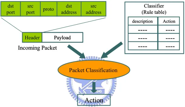
(10) Chapter 1. Introduction. The accelerated growth of Internet applications has increased the importance of the development of new network services, such as security, virtual private network (VPN), quality of service (QoS), accounting, and so on. All of these mechanisms generally require the router to be able to categorize packets into different classes called flows. The categorization function is termed packet classification. An Internet router categorizes incoming packets into flows utilizing information contained in the packet header to lookup the predefined rule table in the router. A rule table maintains a set of rules specified based on the packet header fields, such as the network source address, network destination address, source port, destination port, protocol type and possibly other fields. The rule field can be a prefix (e.g. a network source/destination address), a range (e.g. a source/destination port) or an exact number (e.g. a protocol type). The process of packet classification is presented in Fig. 1. When a packet arrives, the packet header is extracted first and then compared with the corresponding fields of rule in the rule table. A rule matching in all corresponding fields is considered a matched rule. The packet header is compared with every rule in the rule table, and the matched rule with the highest priority yields the best-matching rule. Finally, the router performs an appropriate action associating with the best-matching rule. Table 1 is an example of a rule table. Here, the address fields are shown as 3 bits prefix. A star in address fields indicates a bit mask, and stars for entire entry indicates a wildcard which can be matched by any packet. The port fields are shown with range, and protocol field is shown with exact protocol type, including TCP, UDP and ICMP. Rules are arranged in order of priority. Each rule has an associated action either Deny 1.

(11) or Pass. Consider a packet P with source address of 110, destination address of 010, source port of 4, destination port of 9 and protocol type of TCP arrives. In table1, packet P matches rule 1 and rule 4, where rule 1 has higher priority. Therefore rule 1 is the best-matching rule for packet P. According to the associated action of rule 1, packet P is denied.. dst port. src port. dst address. proto. Header. Classifier (Rule table). src address. description. Action. ----------. ----------. Payload. Incoming Packet. Packet Classification. Action Figure 1: Packet classification process. Rule. Source address. Destination address. Source port. Destination port. Protocol type. Action. 1. 1**. 010. 2-4. 6-9. TCP. Deny. 2. 101. ***. 1-7. 4-6. UDP. Pass. 3. 00*. 10*. *. *. ICMP. Deny. 4. 11*. 01*. 4-8. *. TCP. Pass. 5. ***. ***. *. 10-15. *. Deny. Table 1: An example of packet classification rule table 2.

(12) Longest prefix matching [17] for route lookup is a special case of one-dimensional packet classification. Each rule is described by a prefix (address/mask pair). The length of the prefix defines the priority of the rule. The d-dimensional packet classification problem (PC problem) is formally defined as follows. The rule table has a set of rules R = {R1, R2…, Rn} over d dimensions. Each rule comprises d fields Ri = {F1,i, F2,i…, Fd,i}, where Fj,i denotes the value of field j in rule i. Each rule also has a cost (priority). A packet P(p1,p2…,pd) matches rule Ri if all the header fields pm, m from 1 to d, of the packet match the corresponding fields Fj,i in Ri. If packet P matches multiple rules, the minimal cost (highest priority) rule is returned. The general packet classification problem can be viewed as a point location problem in multidimensional space [1]. Rules have a natural geometric interpretation in d dimensions. Each rule Ri can be considered a “hyper-rectangle” in d dimensions, obtained by the cross product of Fj,i along each field. The set of rules R thus can be considered a set of hyper-rectangles, and a packet header represents a point in d dimensions. Point location in computational geometry involves from a set of non-overlapping objects (hyper-rectangles) finding the enclosing object that a point belongs to. The low bounds for point location problem in N objects with d dimensions, where d > 3, are either an Ο(log N ) time complexity with Ο( N d ) space complexity; or an Ο((log N ) d −1 ) time complexity with Ο(N ) space complexity. However, the packet classification problem allows objects (rules) overlapping with each other. Therefore, packet classification problem is at least as hard as point location problem. A solution of packet classification problem either requires an enormous storage space or long search time. For example, let us assume that we would like the router to be able to process 1,000 rules of 5 dimensions. An algorithm with Ο(log 4 N ) execution time 3.

(13) and Ο(N ) space requires 10,000 memory accesses per packet. This is impractical with any current technology. If we use a Ο(log N ) time and Ο( N 5 ) space algorithm, the space requirement becomes prohibitively large, in the range of 1, 000G bytes. The complexity drives us to use heuristic algorithm being a practical solution for the packet classification problem. By exploiting the characteristic in rule table, heuristic algorithms may break the performance low bound achieved in the point location problem. A good packet classification algorithm must classify packets quickly with minimal memory storage requirements. This study proposes a novel bit compression packet classification algorithm. This algorithm succeeds in reducing the memory storage requirements in the bitmap intersection algorithm [8], proposed by Lakshman and Stiliadis. The bitmap intersection algorithm converts the packet classification problem into a multidimensional range lookup problem and constructs bit vectors for each dimension. Since the bit vectors contain lots of ‘0’ bits, the bit vectors could be compressed. We compress the bit vectors by preserving only useful information but removing the redundant bits of the bit vectors. An additional index table would be created to keep tract of the rule number associated with the remaining bits. Additionally, the wildcarded rules also enable more extensive improvement. The bit compression algorithm reduces the storage complexity from O( dN 2 ) of the bitmap intersection algorithm to O(dN·logN), where d denotes the number of dimensions and N denotes the number of rules, without sacrificing the classification performance. The rest of the thesis is organized as follows. Chapter 2 introduces performance metrics and related works for packet classification problem. Then, the basic idea of compressed bit vector (CBV) and the details of the bit compression algorithm are purposed in Chapter 3. We display experimental platform and the performance results in Chapter 4. And finally, the conclusion and future work is given in Chapter 5. 4.

(14) Chapter 2. Performance Metrics and Related Works. 2.1 Performance Metrics for Packet Classification Algorithm. The packet classification problem has been studied extensively in recent years. A good packet classification algorithm requires taking the following properties into consideration. 1. Search speed The goal of packet classification is to classify packets at wire speed. Currently, Internet links operate at very high speeds. Routers and intrusion detection devices that operate at OC-768 (40Gbps) and even faster link speed have been developed. For example, links running at OC-768 can transmit 125 million packets per second (assuming minimum 40 bytes IP packet) which requires the packet classification engine to process same amount of packets per second. 2. Storage space The amount of memory needed to store the rule table should be small for the cost reason. The small memory requirement allows the use of faster but typically more expensive memory technologies for achieving higher performance. For example, on-chip SRAM provides fast memory access but small storage space. We would ideally like the memory requirement of a packet classification algorithm to scale below the size of an on-chip SRAM for high speed implementations. 3. Update Each time the rule table changes, the data structure needs to be updated. The update rate varies among different applications. For example, emerging applications such as QoS involve dynamically identifying flows, the rules require 5.

(15) fast update. In contrast, the firewall applications can tolerate update infrequently because rules are rarely changed. A packet classification algorithm with fast update prefers especially for the applications requiring frequent rule change. 4. Scalability of number of fields Internet applications differ on the number of fields of the IP header that is used for classification. A good packet classification algorithm must be able to scale the number of fields in order to avoid being outdated by future Internet developments. 5. Flexibility of specification of filed The rule specification should be general and sufficiently expressive to specify various types of header fields. A good packet classification algorithm must support rules involving exact, prefix and range representation.. 2.2 Related Works. Extensive collection of papers [2-15] and numerous approaches have been proposed to solve the packet classification problem. This section describes some of these approaches briefly. Linear search Linear search is the simplest classification algorithm. It is efficient in terms of memory, but for large number of rules this approach implies a large search time. The data structure is simple and easy to be updated as rules change. Hierarchical tries A hierarchical trie (also called multilevel tire or backtracking trie) is a simple extension of the one dimension radix trie data structure. Hierarchical trie is constructed field by field recursively. At beginning, according to first field of each. 6.

(16) rule, construct the first level trie. And then, construct the second level trie from the leaf node on the first level trie. Build the remaining fields recursively. Because of the characteristic of recursive traversal, this scheme suffers long search time. Set-pruning tries The set-pruning trie [12] is similar to hierarchical trie, but with reduced query time obtained by replicating rules to eliminate recursive traversal. Rules are replicated to ensure every packet will encounter matching rules in one path without backtracking. Set-pruning trie successfully reduces search time in hierarchical tries, but unfortunately this scheme has a memory explosion problem which makes it impractical when the size of rule table becomes large. Grid of tries The grid of tires data structure, proposed by Srinivasan et al. [2] reduces storage space by allocating a rule to only one trie node as in a hierarchical trie, and achieves the same search time with set pruning trie by pre-computing and storing a switch pointer which guides the search process in some nodes. This is a good solution if the rules are restrict to only two fields, but is not easily extended to more fields. Hi-Cuts (hierarchical intelligent cuttings) HiCuts [5] attempts to partition the search space in each dimension, guided by simple heuristics that exploits the structure of the rule table. A decision tree data structure is built by carefully preprocessing the rule table. Each time a packet arrives, the decision tree is traversed to find a leaf node, which stores a small number of rules. A linear search of these rules yields the desired matching. While this scheme seems to exploit the characteristics of real rule table, the characteristics vary, however. How to find the suitable decision tree prevents it from scaling well to large rule table. Hyper-Cuts HyperCuts [7] is a similar approach to HiCuts, but uses multidimensional cuts at each 7.

(17) step. Unlike HiCuts, in which each node in the decision tree represents a hyperplane, each node in the HyperCuts decision tree represents a k-dimensional hypercube, where k > 1. HyperCuts appears to have excellent lookup performance. It has excellent storage efficiency in many cases, but does not fare quite as well with heavily wildcarded rules. Tuple Space Tuple space algorithm [3] partitions the rules into different tuples categories based on the number of specified bits (don’t care bits) in the rules, and then uses hasing among rules within the same tuple. This algorithm has fast average search time and fast update time. The main disadvantage of tuple space algorithm is the use of hashing leading to lookups or updates with non-deterministic duration. Cross-producting Cross-producting approach [2] builds a table of all possible field value combinations (cross-products) and pre-computes the best-matching rule for each cross-product. Search can be done quickly by doing separate lookups on each field, pasting the results together into a cross-product, and then indexing into the cross-product table. Unfortunately, the size of cross-product table grows enormously with the number of rules and number of fields RFC (Recursive Flow Classification) RFC [4] is one of the earliest of the heuristic approaches. RFC attempts to map S bits packet header into T bits identifier, where T = log N (N is number of rules) and T<<S. RFC uses crossproducting in stages, and groups intermediate results into equivalence classes to reduce storage requirements. RFC appears to be a fast classification algorithm; this speed, however, comes at the cost of substantial memory usage, and it does not support an efficient updating process. TCAM (Ternary Content Addressable Memory) 8.

(18) TCAM is a hardware device performing the function of a fully associative memory. In TCAM, cells can be stored with three types of value: ‘0’, ‘1’ or ‘X’, where ’X’ represents don’t care. ‘X’ can be operated as a mask representing wildcard bits. Therefore, excluding range match, TCAM can supports exact or prefix match. Range must be transformed to prefix or exact value (e.g. the range gt 1023 can be expressed with 6 prefixes 000001*, 00001*, 0001*, 001*, 01* and 1*). TCAM compares a packet to every rule simultaneously. Packet classification based on TCM is suitable for small rule tables. For large rule table however, using TCAM requires large amount of board space and power consumption and expensive cost. Bit-map intersection The bit-map intersection algorithm devised by Lakshman et al. [8] uses the concept of divide-and-conquer, dividing the packet classification problem into k sub-problems, and then combining the results. This scheme uses the geometrical space decomposition approach to project every rule on each dimension. For N rules, a maximum of 2N+1 non-overlapping intervals are created on each dimension. Each interval is associated with an N-bits bit vector. Bit j in the bit vector is set if the projection of the rule range corresponding to rule j overlaps with the interval. On packet arrival, for each dimension, the interval to which the packet belongs is found. Taking conjunction of the corresponding bit vectors in each dimension to a resultant bit vector, the highest priority entry in the resultant bit vector can be determined. Since the rules in the rule table are assumed to be sorted in terms of decreasing priority, the first set bit found in the resultant bit vector is the highest priority entry. The rule corresponding to the first set bit is the best matching rule applied to the arriving packet. This scheme employs bit-level parallelism to match multiple fields concurrently, and can be implemented in hardware for fast classification. However, this scheme is difficult to apply to large rule tables, since the memory storage scales 9.

(19) quadratically each time the number of rules doubles. The same study describes a variation that reduces the space requirement at the expense of higher execution time. Consider the simple example of a 2-dimensional rule table with four rules, shown in Fig. 2, to illustrate the functioning of the bitmap intersection. The four rules are represented as 2-dimensional rectangles. The construction process of bitmap starts at projecting the edges of the rectangles to the corresponding axes, X axis and Y axis. The four rectangles then create seven intervals in X axis and six intervals in Y axis. Subsequently, each interval is associated with a bit vector. Assume a packet, denoted by a point p in Fig. 2, arrives. The first step of classification is to locate the intervals that contain packet p in both axes. The intervals are X3 and Y2 for X and Y axis respectively. Then read the associated bit vectors of intervals X3 (“1011”) and Y2 (“0011”) respectively. After taking conjunction of these two bit vectors, the resultant bit vector “0011” is built. Obviously, rule 3 is the best matching rule applied to the arriving packet p.. 0. 0. 0. 1. Y6. 0. 1. 0. 1. Y5. 1. 1. 1. 1. Y4. 1. 0. 1. 1. Y3. 0. 0. 1. 1. Y2. 0. 0. 1. 0. Y1. 2. 4. 1 3 P. 1 2 3 4 1 2 3 4. X1. X2. X5. X6. 1. 1. X3 1. X4 1. 1. 1. 1. 0. 0. 0. 0. 1. 1. 0. 0. 0. 1. 1. 1. 0. 0. 0. 1. 1. 0. 0. 0. 0. Figure 2: An example of bitmap intersection algorithm. 10. X7.

(20) ABV (Aggregated Bit Vector) The Aggregated Bit Vector (ABV) algorithm [9] is an improvement on the bit map intersection scheme. The authors propose two observations: there are sparse set bits in bit vectors and a packet matches few rules in the rule table. Building on these two observations, two key ideas are extended, aggregation of bit vectors and rule rearrangement. Aggregation attempts to reduce memory access time by adding smaller bit vectors called ABV (Aggregate Bit Vector), which partially captures information from the whole bit vectors. The length of an ABV is defined as ⎡N A⎤ , where A denotes aggregate size. Bit i is set in ABV if there is at least one bit set in group K, from (i×A)th bit to ((i+1)×A－1)th bit, otherwise bit i is cleared. Aggregation reduces the search time for bitmap intersection, but produces another unfavorable effect, false match, a situation in which the result of conjunction of all ABV returns a set bit, but no actual match exists in the group of rules identified by the aggregate. False matching may increase memory access time. Rule rearrangement can alleviate the probability of false matching. Although ABV outperforms bit map intersection for memory access time by an order of magnitude, it does not ameliorate the main problem of bit map intersection, exponentially growing memory space, yet uses more space.. 11.

(21) Chapter 3. Bit Compression Algorithm. 3.1 Using Bit Compression to Reduce Storage Space As mentioned in the previous section, bit-map intersection is a hardware oriented scheme with rapid classification speed, but suffers from the crucial drawback that the storage requirements increase exponentially with the number of rules. The space complexity of bit-map intersection is O(dN 2), where d denotes the number of dimensions and N represents the number of rules. Even though the ABV algorithm improves the search speed, but requires even more memory space than bitmap intersection algorithm. For a hardware solution of packet classification, memory storage is an important performance metric. Decreasing the required storage will reduce costs correspondingly. The question thus arises whether any method exists way of solving the extreme memory storage of a large rule table. Observing the bit vectors produced by each dimension, as mentioned in [9], the set bits (“1” bits) are very sparse in the bit vectors of each dimension, there are considerable clear bits (“0” bits). The authors of [9] used this property to reduce memory access time, but this property can also be applied to reduce memory storage requirements. For the example of Fig. 4, an approximately 60% space saving can be achieved by removing redundant ‘0’ bits. The shaded parts of Fig. 4 illustrate the removable ‘0’ bits. Therefore, our challenge is how to represent compressed format of bit vector. We try to segment each dimension into several sub-ranges. We call the sub-range “Compressed Region” (CR), where a CR denotes the range of a series of consecutive intervals. In each CR, only an extreme small number of rules are overlapped, while the corresponding bits of the non-overlapped rules in this CR are all 0 bits. If a packet falls into a CR, denoted by CRm, only the overlapped rules need to be taken into 12.

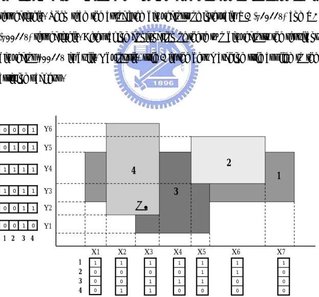
(22) consideration, while the non-overlapped rules do not. The corresponding bits of the non-overlapped rules in CRm are all 0 bits. Neglecting the non-overlapped rules means these 0 bits corresponding to the non-overlapped rules of the bit vectors in CRm can be removed. This study calls the bit vector after removing redundant 0 bits CBV (Compressed Bit Vector). For example, consider the two dimensional rule table like Fig. 3. By dividing dimension X into four CRs, CR1, CR2, CR3 and CR4. Only R1, R3 and R4 are overlapped with CR1. Therefore, if a packet falls into CR1, only R1, R3 and R4 have to be considered. Consequently, maintaining the first, third and forth bits of the bit vectors while removing the ‘0’ bits of the non-overlapped rules in CR1 are sufficient to looking for matching rules. However, recall that in the bit map intersection the bit order of a bit vector indicates to the rule order (i th bits in a bit vector corresponds to i th rule in rule table). ‘0’ bits are removed from a bit vector in such a way that it is no longer known which remaining bits represent what rules. To solve this problem, this study claims an “index list” with each CR, which stores the rule number associated with the remaining bits. Collections of the “index list” form an “index table”. For example in Fig. 3, after removing the redundant 0 bits, the bit vectors in CR1 remain three bits. In order to keep track of the rule number of the three remaining bits, an index list [1, 3, 4] is appended in CR1. Each CR associates an index list, and the index table comprising four index lists shows in Fig. 6. After removing redundant 0 bits, we build the CBVs and index list for each CR. Because the length (number of bits) of CBV is related to the number of overlapped rules in the corresponding CR, the length of the CBVs is different for each CR, For example as Fig. 4, the length of CBVs in CR1 should be three bits, while the length of CBVs in CR2 should be five bits. However, the bit-map intersection is a 13.

(23) hardware-oriented algorithm, and our improvement scheme is also hardware-oriented. For convenience of memory access, the length of bit vectors should be fixed, and thus CBVs maintaining fixed length are also desired. Therefore, the length of all CBV should be based on the longest (maximum bits) CBV, and fill up ‘0’ bits to the end of the CBVs which are shorter than the longest CBV. Notably, a similar idea is applied to the index lists, where the index lists should have the same number of entries.. Y. 1. 9. 2. 3. 6. 8. 10 4. 7 5. CR1. 1 2 3 4 5 6 7 8 9 10. CR2. CR3. X1. X2. X3. X4. X5. X6. X7. X8. 1 0 0 0 0 0 0 0 0 0. 1 0 1 1 0 0 0 0 0 0. 1 0 1 0 0 0 0 0 0 0. 1 1 0 0 1 0 0 1 0 0. 1 1 0 0 1 1 0 1 0 0. 1 1 0 0 0 1 1 0 0 0. 1 0 0 0 0 0 0 0 0 0. 0 0 0 0 0 0 0 0 1 0. CR4. X9. X. 0 0 0 0 0 0 0 0 1 1. Figure 3: The bitmap in dimension X of a 2-dimensional rule table with 10 rules.. Y. 1. 9. 2. 3. 6. 8. 10 4. 7 5. CR1 X. X1 1 2 3 4 5 6 7 8 9 10. 1 0 0 0 0 0 0 0 0 0. 2. 1 0 1 1 0 0 0 0 0 0. CR2. CR3 X. X3. X4. X5. X6. 1 0 1 0 0 0 0 0 0 0. 1 1 0 0 1 0 0 1 0 0. 1 1 0 0 1 1 0 1 0 0. 1 1 0 0 0 1 1 0 0 0. 7. 1 0 0 0 0 0 0 0 0 0. X8 0 0 0 0 0 0 0 0 1 0. CR4. X9. X. 0 0 0 0 0 0 0 0 1 1. Figure 4: Space saving by removing redundant ‘0’ bits. 14.

(24) Furthermore, rules are considered to have wildcards. This study notes that if rule Ri is wildcarded in dimension j, the i th bit of each bit vector in dimension j is set, therefore forms a series of ‘1’ bits over dimension j. For example, Fig. 5 illustrates the rule table with two wildcarded rules in dimension X, rule R11 and R12. The last two bits of each bit vector are set because the ranges of R11 and R12 cover all intervals in dimension X. In [9], the authors mentioned that in the destination and source address fields, approximately half of rules are wildcarded. Consequently, half of each bit vector in the destination field (or source field) is set to ‘1’ owing to wildcards. Intrinsically, lots of these ‘1’ bits are redundant. The idea is that for each dimension j, regardless of the interval that a packet falls in, the packet always matches the rules with wildcards in dimension j. Thus there is no need to set corresponding ‘1’ bits in every interval for recording these wildcareded rules, and instead these rules are stored just once. Additional bit vectors, here called “Don’t Care Vectors” (DCV), are utilized to separate the wildcarded and non-wildcarded rules. A DCV is established for each dimension. Removing the redundant ‘1’ bits caused by wildcarded rules helps further reduce storage space. A DCV resembles a bit vector. Note that in a bit vector, bit j in the bit vector is set if the projection of the rule region corresponding to rule j overlaps with the related interval. In the DCV, bit j is set if the corresponding rule j is wildcarded, otherwise bit j is clear. For example, the last two bits of each bit vector in Fig. 3 could be removed and DCV “000000000011” added instead, which indicates that the 11th and 12th rules are wildcarded and others are not. Using the above ideas, this study proposed an improved approach of bitmap intersection, called “bit compression”. Before describing the proposed bit compression scheme, this study presents some denotations and definitions.. 15.

(25) Y. 1. 9. 2. 3. 6. 8. 10 4. 7. 11. 5. CR1 X 1. 1 2 3 4 5 6 7 8 9 10 11 12. 1 0 0 0 0 0 0 0 0 0 1 1. X2. X3. 1 0 1 1 0 0 0 0 0 0 1 1. 1 0 1 0 0 0 0 0 0 0 1 1. 12. CR2 X 4. 1 1 0 0 1 0 0 1 0 0 1 1. X5. CR3 X 6. 1 1 0 0 1 1 0 1 0 0 1 1. 1 1 0 0 0 1 1 0 0 0 1 1. X7. X8. 1 0 0 0 0 0 0 0 0 0 1 1. 0 0 0 0 0 0 0 0 1 0 1 1. CR4. X9. X. 0 0 0 0 0 0 0 0 1 1 1 1. Figure 5: The bitmap in dimension X of a 2-dimensional rule table which has two wildcarded rules R11 and R12 in dimension X.. For a k-dimensional rule table with N rules, let Ii,j denotes the i th non-overlapping interval on dimension j and ORNi,j denotes the overlapped rule numbers for each interval Ii,j. Furthermore, BVi,j denotes the bit vectors associated with the interval Ii,j and CBVi,j represents the corresponding compressed bit vector. Finally, DCVj is the “Don’t Care Vector” for dimension j and DCVi,j is the i th bit in DCVj. Definition: For a k-dimensional rule table with N rules, “maximum overlap” for dimension j, denoted as MOPj, is defined as the maximum ORNi,j for all intervals in dimension j. The preprocessing part of bit compression algorithm is as follows. For each dimension j, 1 ≤ j ≤ k, 1. Construct DCVj. For n from 1 to N, if RN is wildcarded on dimension j then DCVn,j is set, otherwise DCVn,j is clear. 2. Calculate the value of MOPj and segment the entire range of dimension j into t CRs, CR1, CR2, …, CRt . The rules, where the rule projection overlaps with CRi, 1 16.

(26) ≤ i ≤ t, form a rule set RSi, where the entry number of each rule set should be smaller than or equal to MOPj. (according to the subsequently described “region segmentation” algorithm) 3. For each CR CRi, 1 ≤ i ≤ t, construct a compressed bit vector and corresponding index list based on RSi. Then gather the index lists to compose an index table. Furthermore, use listi to denote the index list related to CRi and listx,i to represent the x th entry of listi. 4. For each CR CRi, 1 ≤ i ≤ t, append “index table lookup address” (ITLA), which is the binary of (i-1), in front of each CBV. For convenient hardware processing, the number of bits of ITLA in each CR are all the same.. The classification steps of a packet are as follows. For each dimension j, 1 ≤ j ≤ k, 1. Find the interval Ii,j to which the packet belongs and obtain the corresponding compressed bit vector CBVi,j and ITLA. 2. Use ITLA to look up the index table to obtain the corresponding index list, assume listm. 3. Read the DCVj into the final bit vector. Subsequently, read the index list found in step 2 entry by entry. If the x th bit in CBVi,j is ‘1’, then access listx,m and set the corresponding bit in the final bit vector. 4. Take the conjunction of the final bit vector associated with each dimension and then determine the highest priority rule implied to the packet.. Figure 6 illustrates the bit compression algorithm. First, construct the DCV “000000000011” for dimension X. As shown in Fig. 1, the dimension X is divided into 4 CRs. In CR1, the corresponding rule set RS1 is {R1, R3, R4}, and thus the CBV in CR1 is constructed by considering R1, R3, R4 only and the index list list1 is [1, 3, 4]. An 17.

(27) ITLA “00” then is appended in front of the CBVs in CR1. As mentioned previously, additional ‘0’ bits are filled up in the CBVs and index table for the convenience of hardware implementation. Furthermore, similar steps are manipulated for CR2, CR3 and CR4.. Index table. 1. P 3. 9. 2 6. 8. 4. 10 7. 5. CR1 CR2 X1 X2 X3 X4 X5 0 0 1 0 0 0 0. 0 0 1 1 1 0 0. 0 0 1 1 0 0 0. 0 1 1 1 1 0 1. 0 1 1 1 1 1 1. 11 12. CR3 X6 X7. X8. 1 0 1 1 1 1 0. 1 1 1 0 0 0 0. 1 0 1 0 0 0 0. CR4 X9 1 1 1 1 0 0 0. Compressed bit map. 00. 1. 3. 4. 0. 0. 01. 1. 2. 5. 6. 8. 10. 1. 2. 6. 7. 0. 11. 9. 10. 0. 0. 0. 1. 1. 1. ITLA. Set bit_1 =1. Don’t Care Vector. Set bit_2 =1. Set bit_5 =1. 0. 1 Set bit_8 =1. 0 0 0 0 0 0 0 0 0 011. 1 1 0 0 1 0 0 1 0 011. Figure 6: An example of bit compression algorithm.. Consider an arriving packet p shown in Fig. 6, which falls into interval X4. The ITLA “01” and CBV “11101” associated with X4 thus are accessed. The ITLA “01” serves as the lookup address in the index table to access index list [1, 2, 5, 6, 8]. The bits of “11101” then are known to represent R1, R2, R5, R6 and R8 respectively. Read DCV “000000000011” and set the first, second, fifth and eighth bits to form the final bit vector. The final bit vector in dimension X is “110010010011”, the same as the bit vector of interval X4 produced by the bitmap intersection scheme in Fig. 5. Similar processes are operated to form the final bit vector of dimension Y. Take the conjunction of the final bit vectors in dimension X and Y, and then the matched highest priority rule is obtained.. 18.

(28) 3.2 Measurement of Maximum Overlap. Because the bit compression scheme does not vary the number of bit vectors, the storage space saving is influenced by the length of the CBV, shorter CBV length leads greater space saving. However, as mentioned previously, the length of the CBV is limited by the value of maximum overlap. Consequently, the space saving increases with decreasing value of the maximum overlap. Notably, the bit compression scheme requires extra storage for the index table. If the value of the maximum overlap is sufficiently large, the overhead for the index table may exceed the profit from compression. To ensure the redundant 0 bits removed from bitmap are large enough to exceed the extra storage overhead (index table) in the bit compression algorithm, this study performs experiments on the destination field to measure statistics of the maximum overlap. This study employs two approaches to create the one-dimensional rule table with 0.5K, 1K, 5K and 10K numbers of rules. In the first approach, the rule tables are generated by randomly picking prefixes from Mae-West routing database [22]. In the second approach, the type of rule table considers the prefix length distribution probability based on five publicly available routing tables in [9] and probability, β, [10], which denotes the probability that prefix PA is a prefix of prefix PB, where PA and PB are randomly selected from the rule table. β is an important parameter for the second rule type for controlling rule overlapping probability, and overlapping probability increases with increasing β. In [10], the authors calculated the value of β and acquired results about 10-5 for several real-life routing tables obtained from the Mae-West routing database. This study considers four different values of β (10-2, 10-3, 10-4 and 10-5). Table 2 and 3 present the statistical results of first and second approach 19.

(29) respectively. The maximum and average values of maximum overlap of 1000 statistics are calculated. For real-life Mae-west routing tables, the ratio of maximum overlap to rule numbers shown in table 2 is low (below 0.006). And for rule tables created by second approach, as expected, maximum overlap increases with β. Table 3 shows that even with large β, the ratio of maximum overlap to rule numbers still remains low (below 0.044). The statistics confirm that considerable storage in the bitmap intersection is saved through bit compression. Notably, the maximum overlap for Mae-west routing table lie between the statistical results of the second approach with β=10-4 and β=10-5. Number of Rules. Max.. Average. 0.5K. 3. 2.111. 1K. 4. 2.561. 5K. 7. 4.734. 10K. 9. 6.58. Table 2: The statistical maximum and average value of “maximum overlap” for real-life Mae-West routing table. β＝10-2. β＝10-3. β＝10-4. β＝10-5. Number of Rules Max.. Average. Max.. Average. Max.. Average. Max.. Average. 0.5K. 22. 15.308. 7. 4.827. 4. 2.544. 3. 2.014. 1K. 36. 25.879. 10. 6.777. 6. 3.205. 4. 2.119. 5K. 114. 98.39. 26. 18.183. 9. 5.844. 5. 3.158. 10K. 253. 189.075. 42. 29.487. 11. 8.178. 6. 3.742. Table 3: The statistical maximum and average value of “maximum overlap” for different β 20.

(30) 3.3 Region Segmentation Algorithm. This section describes the “region segmentation” algorithm. As mentioned previously, the region segmentation algorithm is used to segment the range of each dimension into CRs and then to groups rules overlapping with each CR. Moreover, since in bit compression algorithm, each CR is associated with an index list which contains the same number of entries (the maximum overlap). So, if more CRs are constructed, more storage space is needed to store the index list. Minimizing the number of CR can help bit compression algorithm save space further. Consequently the objective of region segmentation algorithm is to segment the range of dimension into minimum number of CRs such such that the number of rules overlapping within each CR is smaller than or equal to the maximum overlap. The region segmentation algorithm transforms this problem into a graph model according to the rule dependency. The definition of rule dependency is as follows. Definition: Projecting all rule regions to one dimension, rules Ri and Rj are considered dependent if they overlap, and otherwise are considered independent. According the rule dependency, the region segmentation algorithm constructs a undirected graph G (V, E) first, where V = {v1,v2, …, vN}, each vertex vi corresponds to a rule Ri, and an edge is constructed between vi and vj if rules i and j are dependent. Graph G would include several connected components, where each connected component represents a group of mutually dependent rules that form a separated CR. The corresponding rules of a connected component form a rule set. If the vertex numbers of connected component (rule numbers of rule set) are less than or equal to the maximum overlap, the connected component (rule set) is desired; otherwise the maximum degree vertex (which means neglect the rule overlapped with maximum number of rules) and the related edges are removed, and the search for desired 21.

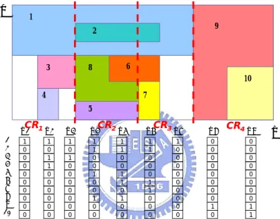
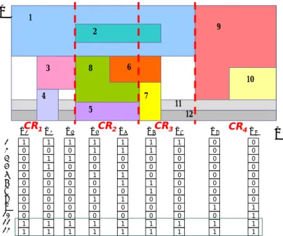
(31) connected components continues. In fact, the rule set corresponding to a connected component should consider the removed vertexes originally connected with the connected component. The process is repeated until the vertex numbers of each connected component are less than or equal to the maximum overlap. For example, Fig. 7(a) presents a graph model constructed using the rule table of Fig. 1, in which the maximum overlap equals 5. First, two connected components, C1 and C2, are found, as shown in Fig. 7(b). The corresponding rule set of C2 is {R9, R10}, where the numbers of rule are 2, less than maximum overlap, and thus the rule set is desired. On the other hand the rule set corresponding to connected component C1 has eight vertexes, so the maximum degree vertex of C1, vertex v1, and the related edges are removed. Subsequently, two new connected components, C11 and C12, are obtained, as shown in Fig. 7(c). The corresponding rule set of C11 and C12 should take R1 into consideration, therefore the rule set of C11 should be {R1, R3, R4} and the rule set of C12 should be {R1, R2, R5, R6, R7, R8}. {R1, R3, R4} is a desired rule set, while the maximum degree vertex, v2, is neglected for C12 and the process is continued like Fig. 7(d) and 7(e). Finally, four desired rule sets {R1, R3, R4}, {R1, R2, R5, R6, R8}, {R1, R2, R6, R7} and {R9, R10} are obtained. The region segmentation algorithm achieves the objective for minimizing the number of CRs by merging the rule sets. Two rule sets can be merged together if the rule numbers of the merged rule set are still smaller than or equal to the maximum overlap. The merged CRs then share the same index list. After merging the rule set, the required number of index lists can be reduced such that the space of the index table is saved. For example, Fig. 8 merges the rule set {R1, R3, R4} and {R9, R10}, so CR1 and CR4 can be considered as the same CR which uses only an index list [1, 3, 4, 9, 10]. The CBVs in regions 1 and 4 then employ ITLA “00” to access the same index list. Comparing with Fig.6, merging rule sets helps the index table in Fig. 8 save 1/4 storage space. 22.

(32) 1. remove. 10. 2. 1. 10. 2. C2. 9 3. 9 3. 8. 4. 4. 7 5. 8. 7. C1. 6. 5. 6. Figure 7(a). Figure 7(b). remove. 10. 1. 2 9 3. 8. C11 4. 7 5. 6. C12. Figure 7(c) 1. 1. 10. 2. 2. 9 3. 9 3. 8. 4. 10. 7. 8. 4. 7. 6. 5. 5. remove. Figure 7(d). 6. Figure 7(e). Figure 7: Graph model illustrating the steps of the region segmentation algorithm. In order to observe the performance of region segmentation algorithm with merging rule set, we compare the number of CRs constructed by merging rule sets with the low bound. The low bound for the number of CRs is determined by the number of rules and maximum overlap, since the maximal number of rules in each CR is equal to maximum overlap. Therefore the low bound of the number of CRs for 23.

(33) N-rules rule table is N. MOPj. . Figure 9 presents the statistical results under three. different β (10-3, 10-4 and 10-5). The number of CRs constructed by region segmentation with merging rule sets is very close to the low bound.. 1. 3. X1. 0 0 1 0 0 0 0. 6. 0 0 1 1 0 0 0. CR2. 10 7. 5. X2 X3. 0 0 1 1 1 0 0. Index table. 8. 4 CR1. 9. 2. 11 12. X4. X5. X6. 0 1 1 1 1 0 1. 0 1 1 1 1 1 1. 1 0 1 1 1 1 0. CR3. X7. X8. 1 0 1 0 0 0 0. 0 0 1 0 0 0 0. 00. 1. 3. 4. 9. 10. 01. 1. 2. 5. 6. 8. 10. 1. 2. 6. 7. 0. CR4. X9. 0 0 1 1 0 0 0. Figure 8: An example of bit compression algorithm after merging rule sets. 2500. number of CRs. 2000 1500 1000 500 0 1K. 2K. 3K. 4K. 5K 6K number of rules. low bound (β=0.001) low bound (β=0.0001) low bound (β=0.00001). 7K. 8K. 9K. 10K. merge rule set (β=0.001)" merge rule set (β=0.0001) merge rule set (β=0.00001). Figure 9: Performance comparison of number of CRs between low bound and region segmentation with merging 24.

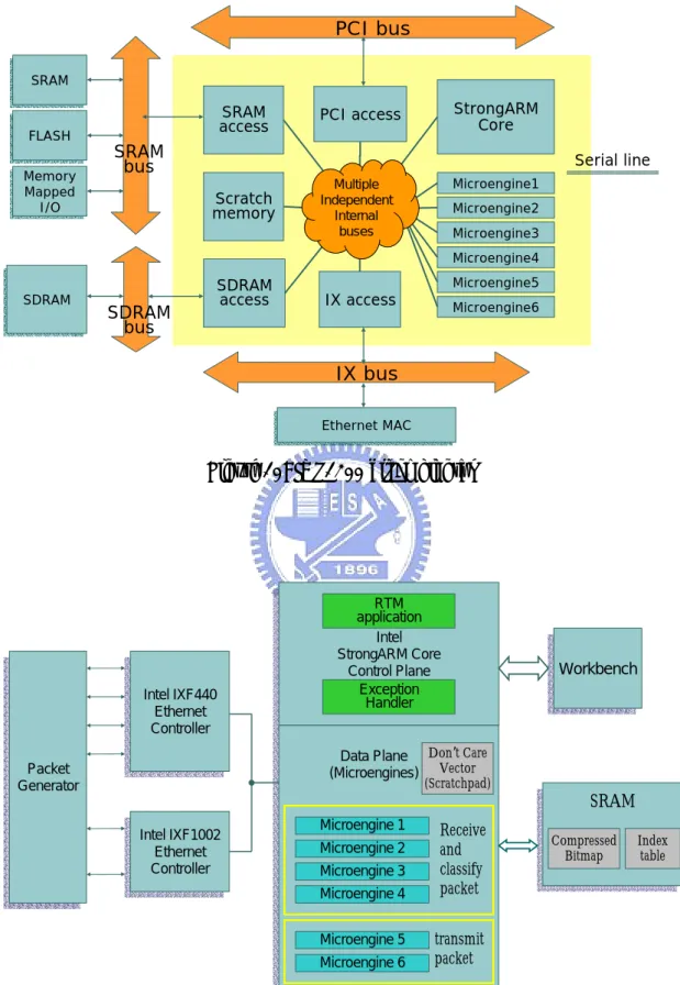
(34) Chapter 4. Performance Results. 4.1 Performance Analysis. For a d-dimensional rule table with N rules, the query time of our bit compression scheme contains the time to do interval lookup, denoted by TIL, and the time to access ITLA, CBV, index list and don’t care vector from memory storage. The time complexity should be O (d ⋅ (TIL + (log r + n + n log N + N ) W )) , where r is the number of index lists, n is the value of maximum overlap and W is the memory bandwidth, while the time complexity of bitmap intersection is O (d ⋅ (TIL + N W )) . The space requirement of bit compression contains four parts -- ITLA, CBV, index table and don’t care vector. We neglect the space complexity of don’t care vector because the size of it is much less than the other three parts. The space complexity is O (d ⋅ N ⋅ (log r + n + log N )) the storage complexity is reduced roughly by a factor of N comparing with the complexity O ( d ⋅ N 2 ) of bitmap intersection.. 4.2 Experiment Platform. We have implemented the bitmap intersection and bit compression algorithms with Microengine C based on IXP1200 [20]. Experiments are conducted on the Intel IXP1200 Developer WorkBench [21]. At beginning, we closely examine the hardware architecture of IXP1200, as shown in Fig. 10. The 32-bit embedded RISC processor, StrongARM, governs the initialization of the whole system and handles higher layers of the protocol stack as well as any packet 25.

(35) that raises an exception. Six microengines, where each supports 4 hardware threads, form the basis of fast path processing. The microengines are intended to handle low-level transfer among I/O devices and memory as well as basic packet processing tasks such as frame de-multiplexing. The microengines also support zero context switching overhead, and other specifically designed instructions for bit, byte, and longword operations. The memory hierarchy in IXP1200 consists of multiple memories, and three primary memory devices are focused on. First, SRAM is used for storing lookup tables and has facilities that allow the manipulation of stack to hold packet headers or lists of packets forwarding. Second, the largest SDRAM is used for storing mass data of packets. And third, the onboard Scratchpad memory offers fastest access time and serves as a local data store. The 64-bit IX bus interface unit is responsible for servicing MAC interface ports on the IX Bus, and moving data to the receive FIFOs or from the transmit FIFOs. The MAX devices can be either multiple 10/100BT Ethernet MAC, Gigabit Ethernet MAC, or ATM MAC. Figure 11 is our system configuration. We use 4 microengines to receive, classify and route packet and remaining 2 microengines to transmit packet. The StorngARM core handles the routing table management and exception. Three types of memory storage are used, a SRAM configuration of 8MB, a SDRAM of 64MB and a scratchpad memory of 4KB. In bitmap intersection, SRAM or SDRAM is used to store the bit vectors according to the size of required space. And the memory access latency and the bus bandwidth of the three types of memory is Scratchpad: 12~14 clks with 32-bits bus, SRAM: 16~20 clks 32-bits bus and SDRAM: 33~40 clks 64-bits bus respectively. In bit compression scheme, SRAM is used to store compressed bit vectors, index table and scratchpad stores the DCV.. 26.

(36) PCI bus SRAM SRAM. FLASH FLASH Memory Memory Mapped Mapped I/O I/O. SRAM access. PCI access. StrongARM Core. Scratch memory. Multiple Multiple Independent Independent Internal Internal buses buses. Microengine1. SRAM bus. Serial line Microengine2 Microengine3 Microengine4. SDRAM SDRAM. SDRAM bus. SDRAM access. Microengine5. IX access. Microengine6. IX bus Ethernet MAC MAC Ethernet. Figure 10: IXP1200 block diagram. IntelIXF440 IXF440 Intel Ethernet Ethernet Controller Controller. RTM application Intel Intel StrongARM Core StrongARM Core ControlPlane Plane Control Exception Handler DataPlane Plane Don’t Care Data Vector (Microengines) (Microengines) (Scratchpad). Packet Packet Generator Generator IntelIXF1002 IXF1002 Intel Ethernet Ethernet Controller Controller. Microengine 1 Microengine 2 Microengine 3 Microengine 4 Microengine 5 Microengine 6. Receive and classify packet. Workbench Workbench. SRAM SRAM Compressed Bitmap. Index table. transmit packet. Figure 11: IXP 1200 system configuration for 2-dimensional bit compression design. 27.

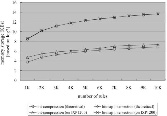
(37) 4.3 Experiment Results. This study considers the complexity of storage requirement and classification performance. We focus on the two dimensional rule table, IP destination address and IP source address. The proposed scheme randomly generates two field rules to create a synthesized rule table, as previous experiments consider the prefix length distribution and β. Recall that for the real-life routing table, the value of β is approximately 10-5 and maximum overlap is measured to be between β=10-4 and 10-5. Therefore, this study lists the experimental performance statistics with β=10-4 and 10-5 and even a larger β, 10-3. Figures 12, 13 and 14 compare the memory requirements (based on log2) for the bit-map intersection and bit compression schemes. Notably, since the bitmap intersection and bit compression use the same size of memory storage to store interval boundary, we omit the memory storage of interval boundary in memory requirements. The experimental results demonstrate that the proposed scheme performs better than bitmap intersection. Under β=10-5, with the rule table size of 5K, we need only 164 Kbytes to store the bit compression algorithm compared with 12.5 Mbytes by bitmap intersection. And with the rule table size of 10K, 374 Kbytes is needed to store the bit compression algorithm compared with 48 Mbytes of bitmap intersection. The memory storage for bitmap intersection scales quadratically each time the number of rules doubles, while bit compression algorithm is almost linear with rule numbers. Bit compression algorithm prevents memory exploration with large rule tables. The difference between theoretical and implementation on IXP1200 is that the lengths of CBV, index list and DCV are a multiple of 32 bits when stored on IXP1200 for convenient memory access, creating a certain amount of space wastage. Therefore, the memory storage with implementation on IXP1200 is higher than the theoretical value. 28.

(38) 16. memory storage (KBs) (based on log2). 14 12 10 8 6 4 2 0 1K. 2K. 3K. 4K. 5K. 6K. 7K. 8K. 9K. 10K. number of rules bit-compression (theoretical) bit-compression (on IXP1200). bitmap intersection (theoretical) bitmap intersection (on IXP1200). Figure 12: Compare the memory requirements (log2 scale) between the bit compression and the bitmap intersection algorithm under β=10-3. 16. memory storage (KBs) (based on log2). 14 12 10 8 6 4 2 0 1K. 2K. 3K. 4K. 5K. 6K. 7K. 8K. 9K. 10K. number of rules bit-compression (theoretical) bit-compression (on IXP1200). bitmap intersection (theoretical) bitmap intersection (on IXP1200). Figure 13: Compare the memory requirements (log2 scale) between the bit compression and the bitmap intersection algorithm under β=10-4 29.

(39) 18. memory storage (KBs) (based on log2). 16 14 12 10 8 6 4 2 0 1K. 2K. 3K. 4K. 5K. 6K. 7K. 8K. 9K. 10K. number of rules bit-compression (theoretical) bit-compression (on IXP1200). bitmap intersection (theoretical) bitmap intersection (on IXP1200). Figure 14: Compare the memory requirements (log2 scale) between the bit compression and the bitmap intersection algorithm under β=10-5. As noted previously, the space of index table can be further reduced by merging the rule sets. Figures 15, 16 and 17 display the total memory space consumed by the rule table of the bit compression scheme with and without merging under. As a result, the required space is reduced about 25%~40% after merging the rule sets.. 30.

(40) Memory Stroage (KBs). before merging. 180 160 140 120 100 80 60 40 20 0. 1K. 2K. 3K. 4K. 5K. after merging. 6K. 7K. 8K. 9K. 10K. Number of Rules Figure 15: The improvement of memory storage by merging rule sets under β=10-3. before merging. after merging. Memory Stroage (KBs). 300 250 200 150 100 50 0. 1K. 2K. 3K. 4K. 5K. 6K. 7K. 8K. 9K. 10K. Number of Rules Figure 16: The improvement of memory storage by merging rule sets under β=10-4. 31.

(41) before merging. after merging. Memory Stroage (KBs). 400 350 300 250 200 150 100 50 0. 1K. 2K. 3K. 4K. 5K. 6K. 7K. 8K. 9K. 10K. Number of Rules Figure 17: The improvement of memory storage by merging rule sets under β=10-5. Besides the bit compression and bitmap intersection schemes, we propose a different compression scheme here, called ACBV (Aggregated and Compressed Bit Vector), which is a modification of the ABV scheme [9]. The ACBV scheme compresses the bit vectors into aggregated and compressed bit vectors. An aggregated and compressed bit vector comprises two parts, aggregated part and compressed part. The aggregated part is an aggregated bit vector of the ABV scheme. The compressed part records sections of bit vector in which have at least one ‘1’ bit. The preprocessing steps of the ACBV scheme are as follows. 1. Aggregate the bit vector to form the aggregated part. Bit i is set in the aggregated part if there is at least one bit set in the bit vector from (i × A). th. (((i + 1) × A) − 1)th. to. bits, otherwise bit i is cleared. A denotes aggregated size.. 2. Construct the compressed part. For i from 0 to ⎡N A⎤ －1, where N denotes the number of rules. If bit i is set in the aggregated bit vector, the section of the bit. 32.

(42) vector from (i × A) to th. (((i + 1) × A) − 1)th. bits is selected. Compact the selected. sections of bit vector together in selecting order to form the compressed part. 3. Append the compressed part to the aggregated part to form the “aggregated and compressed bit vector”. 4. To maintain the same vector length, fill up ‘0’ bits to the end of the aggregated and compressed bit vectors. Figure 18 illustrates the preprocessing steps of the ACBV scheme. Figure 18(a) presents the bitmap of the 2-dimensional rule table. Let’s consider the interval X3. First, the aggregated part is built. We use an aggregate size A=4 in Fig. 18(b). The associated bit vector “10010000” is aggregated to “10” first. Subsequently, according to the aggregated part, select the desired sections of the bit vector. Since the first bit of the aggregated part is ‘1’. The first 4 bits of the bit vector “10010000” are selected to form the compressed part, which is “1001”. Then append the compressed part to the aggregated part, the aggregated and compressed bit vector “101001” is completed. After describing the preprocessing steps, let’s explain how the ACBV scheme classifies the packet. Assume an arriving packet p shown in Fig. 18(b) falling into interval X3. The classification process is as follows. First, the aggregated and compressed bit vector associated with X3 is accessed. The aggregated part “10” indicates the first 4 bits of the bit vector are recorded in the compressed part, while the second 4 bits are not recorded. The second 4 bits of the bit vector is “0000”. Therefore, read the compressed part, we can restore the bit vector to “10010000”. For dimension Y, operate the similar process to restore the bit vector, and take the conjunction of these bit vectors to get best-matching rule. Furthermore, the rule table presented in Fig. 18 doesn’t have wildcarded rules. If the wildcarded rules are considered, the idea of “Don’t Care Vector” of the bit. 33.

(43) compression scheme can be applied.. Y 3 1. 2. X1 X2 0 1 1 0 0 0 0 0. 0 0 1 1 0 0 0 0. 7. 6. 4 1 2 3 4 5 6 7 8. 8. 5. X3. X4. X5. 1 0 0 1 0 0 0 0. 0 0 0 0 1 0 0 0. 0 0 0 0 1 1 0 0. X6 X7 X8 X 0 0 0 0 0 0 0 1. 0 0 0 0 0 0 1 1. 0 0 0 0 0 0 1 0. Figure 18(a). Y 3 2. 1. P. 8. 5. 6. 4 X1 X2. X3. X4. X5. X6. 1 0 0 0 1 1. 1 0 1 0 0 1. 0 1 1 0 0 0. 0 1 1 1 0 0. 0 1 0 0 0 1. 1 0 0 1 1 0. 1 0 1 0 0 1. 7 X7 X8 0 1 0 0 1 1. 0 1 0 0 1 0. X. 1001. 0000. aggregated part. 10010000 compressed part. final bit vector. Figure 18(b) Figure 18: An example of the ACBV scheme. Figure 19 compares the memory requirements (based on log2) for the ACBV, bit compression and bitmap intersection schemes under β=10-5. In the ACBV scheme, we 34.

(44) take 4 different aggregate sizes (8, 16, 32 and 64) into consideration. Under 4 different aggregate sizes, the memory requirements for ACBV scheme are between 638 Kbytes and 1.62 Mbytes for 5K rules and between 1.94 Mbytes and 6.33 Mbytes for 10K rules. Recall that the bitmap intersection requires 12.5 Mbytes and 374 Kbytes for 5K and 10K rules, and the bit compression requires 164 Kbytes and 374 Kbytes for 5K and 10K rules. The experimental results demonstrate that the ACBV scheme performs better than bitmap intersection while worse than bit compression.. 18. Memory Storage (KBs) (based on log2). 16 14 12 10 8 6 4 2 0 1K. 2K. 3K. ACBV, size=8 ACBV, size=64. 4K. 5K 6K Number of Rules. ACBV, size=16 bit compression. 7K. 8K. 9K. 10K. ACBV, size=32 bitmap. Figure 19: Compare the memory requirements (log2 scale) for ACBV, bit compression and the bitmap intersection algorithm under β=10-5. Table 4, 5 and 6 show the worse case memory access times with different number of rules under β = 10-3, 10-4 and 10-5 on IXP 1200. Here, we assume the memory access time is 14, 20 and 40 clks for scratchpad, SRAM and SDRAM respectively. In the bitmap intersection scheme, the rule table is expected to store in SRAM. But the memory storage increases rapidly such that the required storage exceeds the 35.

(45) size of SRAM (8MB). For example, under β = 10-5, the required storage space for the rule table with rules more than 4K exceeds 8MB. Thus the rule table of more than 4K rules must be stored in SDRAM. In the bit compression scheme, the memory exploration is prevented. For 2-dimensional rule table with 10K rules, the bit compression scheme still store the bit vector and index table using SRAM without SDRAM. Moreover, because most memory access cost of the bit compression scheme is expended to access the DCVs, we take advantage of memory hierarchy to store the DCVs in the smallest (4KB) but fastest scratchpad memory rather than SRAM. Storing the DCVs in the scratchpad memory facilitate decreasing memory access time for our bit compression scheme, while the bitmap intersection can only use SRAM or SDRAM. Therefore, although the times of memory access of bit compression are more than bitmap intersection for the same size rule tables, the memory access performance of bit compression is better than bitmap intersection. In the ACBV scheme, we use an aggregate size 32. Under aggregate size 32, the memory requirement is below the size of SRAM for 10K rules. Therefore, SRAM is employed to store the aggregated and compressed bit vectors. Moreover, like the bit compression scheme, the ACBV scheme utilizes the scratchpad memory to stores DCVs. Since an aggregated and compressed bit vector has more bits than the sum of a compressed bit vector and index list. The memory access times of ACBV scheme are more than bit compression scheme. Therefore, the memory access performance of ACBV is worse than bit compression. However the memory access performance is still better than bitmap intersection.. 36.

(46) Number of Rules. bit map intersection. bit compression. ACBV, size=32. No. of Scratchpad access No. of SRAM access No. of SDRAM access Memory access time (clks) No. of Scratchpad access No. of SRAM access No. of SDRAM access Memory access time (clks) No. of Scratchpad access No. of SRAM access No. of SDRAM access Memory access time (clks). 1K. 2K. 3K. 4K. 5K. 6K. 7K. 8K. 9K. 10K. 0. 0. 0. 0. 0. 0. 0. 0. 0. 0. 64. 126. 188. 250. 314. 376. 0. 0. 0. 0. 0. 0. 0. 0. 0. 0. 220. 250. 282. 314. 1280. 2520. 3760. 5000. 6280. 7520. 8800. 10000. 11280. 12560. 64. 126. 188. 250. 314. 376. 438. 500. 564. 626. 10. 14. 16. 18. 24. 26. 28. 30. 32. 34. 0. 0. 0. 0. 0. 0. 0. 0. 0. 0. 1096. 2044. 2952. 3860. 4876. 5784. 6692. 7600. 8536. 9444. 64. 126. 188. 250. 314. 376. 438. 500. 564. 626. 16. 26. 32. 40. 48. 54. 62. 68. 74. 80. 0. 0. 0. 0. 0. 0. 0. 0. 0. 0. 1216. 2284. 3272. 4300. 5356. 6344. 7372. 8360. 9376. 10364. Table 4: Worse case of memory access times under β = 10-3 on IXP1200. Number of Rules. bit map intersection. bit compression. ACBV, size =32. No. of Scratchpad access No. of SRAM access No. of SDRAM access Memory access time (clks) No. of Scratchpad access No. of SRAM access No. of SDRAM access Memory access time (clks) No. of Scratchpad access No. of SRAM access No. of SDRAM access Memory access time (clks). 1K. 2K. 3K. 4K. 5K. 6K. 7K. 8K. 9K. 10K. 0. 0. 0. 0. 0. 0. 0. 0. 0. 0. 64. 126. 188. 250. 0. 0. 0. 0. 0. 0. 0. 0. 0. 0. 158. 188. 220. 250. 282. 314. 1280. 2520. 3760. 5000. 6320. 7520. 8800. 10000. 11280. 12560. 64. 126. 188. 250. 314. 376. 438. 500. 564. 626. 6. 8. 8. 8. 8. 10. 10. 10. 10. 12. 0. 0. 0. 0. 0. 0. 0. 0. 0. 0. 1016. 1924. 2762. 3660. 4556. 5464. 6332. 7220. 8096. 9004. 64. 126. 188. 250. 314. 376. 438. 500. 564. 626. 10. 14. 16. 20. 22. 26. 28. 32. 34. 38. 0. 0. 0. 0. 0. 0. 0. 0. 0. 0. 1096. 2044. 2952. 3900. 4836. 5784. 6692. 7640. 8576. Table 5: Worse case of memory access times under β = 10-4 on IXP1200. 37. 9524.

(47) Number of Rules. bit map intersection. bit compression. ACBV, size =32. No. of Scratchpad access No. of SRAM access No. of SDRAM access Memory access time (clks) No. of Scratchpad access No. of SRAM access No. of SDRAM access Memory access time (clks) No. of Scratchpad access No. of SRAM access No. of SDRAM access Memory access time (clks). 1K. 2K. 3K. 4K. 5K. 6K. 7K. 8K. 9K. 10K. 0. 0. 0. 0. 0. 0. 0. 0. 0. 0. 64. 126. 188. 0. 0. 0. 0. 0. 0. 0. 0. 0. 0. 126. 158. 188. 220. 250. 282. 314. 1280. 2520. 3760. 5040. 6320. 7520. 8800. 10000. 11280. 12560. 64. 126. 188. 250. 314. 376. 438. 500. 564. 626. 6. 6. 6. 6. 6. 6. 6. 6. 6. 6. 0. 0. 0. 0. 0. 0. 0. 0. 0. 0. 1016. 1884. 2752. 3620. 4516. 5384. 6252. 7120. 8016. 8884. 64. 126. 188. 250. 314. 376. 438. 500. 564. 626. 8. 10. 12. 14. 18. 20. 22. 24. 26. 28. 0. 0. 0. 0. 0. 0. 0. 0. 0. 0. 1056. 1964. 2872. 3780. 4756. 5664. 6572. 7480. 8416. 9324. Table 6: Worse case of memory access times under β = 10-5 on IXP1200. As mentioned above, the bit compression and ACBV need less memory access time than bitmap intersection. But notably, compared with bitmap intersection, the bit compression and ACBV algorithm require decompressing a compressed bit vector or aggregated and compressed bit vector to a bit vector. Extra processing time for decompression is required, which will degrade the classification performance. However, the time for decompression is actually much less than memory access time. The memory access time dominates the classification performance. Therefore, even the bit compression and ACBV schemes require extra processing time for decompression. The bit compression and ACBV schemes can still outperform bitmap intersection. Figure 20 presents the packet transmission rates for bitmap intersection, bit compression and ACBV schemes with different size of rule tables without wildcards under β =10-5 on IXP 1200. In the bitmap intersection scheme, the rule tables are stored in SDRAM. In the bit compression and ACBV schemes, the rule. 38.

(48) table is stored in SRAM only. Because the memory access time for reading a CBV and index list or reading an aggregated and compressed bit vector is less than reading a bit vector. Although extra processing time for decompression is required. The bit compression and ACBV schemes outperform bitmap intersection scheme. The transmission rate of the ACBV scheme is between the bitmap intersection scheme and the bit compression scheme. Moreover, since the length of CBVs and index lists almost remain a fixed value (according to maximum overlap), the transmission rate of the bit compression scheme nearly remain constant. In contrast, the transmission rate of bitmap intersection decreases linearly with number of rules.. 500 450 transmission rate (Mbps). 400 350 300 250 200 150 100 50 0 1K. 2K. 3K. 4K. 5K 6K numbers of rule. bitmap intersection (SDRAM). 7K. 8K. bit compression. 9K. 10K. ACBV. Figure 20: Transmission rates for bitmap intersection, bit compression and ACBV on IXP1200. 39.

(49) Chapter 5 Conclusion and Future Work. Packet classification is an essential function of QoS, MPLS and several network services. There are numerous various investigations have addressed this problem. This thesis attempts to improve the original bitmap intersection algorithm, which has memory explosion problem for large rule table. This study introduces the notion of bit compression to significantly decrease the storage requirement, creating what we called the CBV. Bit compression is based on the fact that ‘1’ bits are sparse enabling redundant ‘0’ bits to be removed. By region segmentation, the bit compression algorithm segments the range of dimension into CRs and then associates each CR with an index list. Merging rule sets reducing the number of CRs further. For rule table with wildcared rules, the bit compression propose a novel idea, “Don’t Care Vector” to save plenty storage space. The experiments for measuring maximum overlap led us to believe that plenty of redundant ‘0’ bits exist, such that removing ‘0’ bits can significantly improve memory storage. Compared with bitmap intersection, the storage complexity is reduced from O( dN 2 ) of bitmap intersection to O(dN·logN). In our experiment, our bit compression scheme only needs less than 380 Kbytes to store the 2-dimensional rule table with 10K rules, while bitmap intersection needs 48 Mbytes. Furthermore, comparing with memory access speed, our algorithm accesses average 96% less bits than bitmap intersection. Additionally, by exploiting the memory hierarchy to store the DCV, our bit compression scheme requires much less memory access time than bitmap intersection. Even though extra processing time for decompression is required for bit compression. The bit compression scheme still outperforms bitmap intersection scheme on the classification speed. 40.

(50) Future work on our study is to prove the practicability of our algorithm. We attempt to implement our algorithm on the hardware based platform, such as Intel IXP2400 or FPGA (Field Programmable Gate Array) to verify the practicability of bit compression algorithm. A good packet classification engine also needs to quickly update the algorithm data structure to accommodate the changes in the rule table. In terms of fast update, bitmap requires pre-processing entire rule table each time when the rule changes. However, since our bit compression algorithm segments dimension range into CRs, it is enough to update the bit vectors in CRs which overlapped with changed rule only. In future work, we will investigate exhaustively the update policy of our algorithm. Finally, we will extend our algorithm to support different field of the IP header. In the thesis, we consider the rule table only with layer-3 destination and source address fields. Bit compression algorithm performs well with these two layer-3 address fields. However, does bit compression scheme adapt to other IP header fields? For example, bit compression scheme does not suit for layer-4 protocol type field. Because the protocol type field is restricted to a small set of exact values, such as TCP, UDP, ICMP, etc., the projection of rules in protocol type field are few, which means the probability of rule overlapping is high. Therefore, the maximum overlap in protocol type field would be large. It leads to performance degradation using bit compression scheme. In the future work, we will measure the maximum overlap of layer-4 source port and destination port from real-life rule database. By measure the maximum overlap, we can investigate the adaptation of the bit compression algorithm to layer-4 source port and destination port fields.. 41.