雙Tsuji燃燒器火燄交互作用之實驗與數值分析(I)

(1)

行政院國家科學委員會專題研究計畫成果報告

雙 Tsuji 燃燒器火燄交互作用之實驗與數值分析

（1/2）

The Theoretical and Experimental Studies on

Flame Interaction of Dual Tsuji Burners (1/2)

計畫編號 NSC 90-2212-E-009-048

執行期限九十年八月一日至九十一年七月三十一日

(2)

中文摘要

本計畫主要針對多孔單圓柱上之火焰吹離現象作一完整的數值模擬及實驗觀測。在數值模擬中，本研究將四步化學反應機構導入陳俊勳及翁芳柏兩位教授先前所發展的燃燒模式中。至於實驗儀器方面則包括了風洞及多孔燒結之圓柱形燃燒器，然後吾人就可利用這些儀器來觀察圓柱形燃燒器上的火焰行為，而所探討的參數則包括了進氣速度與注油面積。另一方面，吾人可用數位攝影機將火焰結構及其轉變過程錄下，然後便可將前半面圓柱噴油情況下的火焰依其特性分成四個區域（I-IV），而在全圓柱噴油下則只能分成兩區（V 及 VI）。在第 I 至 III 區中，當進氣速度等於 0.41m/sec 時可在圓柱形燃燒器上形成一個包封火焰，至於火焰所呈現的顏色則是這些區域間的主要差異。在第 IV 及第 V 區中，當進氣速度增加時，包封、尾流、吹離及晚期尾流火焰就會依次出現，另外，由於在全圓柱注油時燃料可以直接噴入吹離火焰中，因此其出現區間遠較前半圓柱噴油時為大。至於第 VI 區的吹離火焰則是緊跟在包封火焰後隨即出現，且在其兩者間並無尾流火焰的存在，之後當進氣速度繼續增加時，尾流火焰仍會接在吹離火焰後出現。另一方面，在數值模擬中，包封擴散火焰、尾流火焰、吹離火焰和尾流火焰在火焰完全熄滅前會隨著進氣速度的增加而依序出現，而當進氣速度為 1.05m/sec 時可產生一 1.7D 的最大吹離高度，且此高度可一直保持至進氣速度達到 1.09m/sec 時，然後吹離

(3)

高度就會隨著進氣速度的增加而逐漸降低，而此一過程即可視為回火。再者，吾人可發現當這些吹離火焰出現時，於圓柱形燃燒器的後方並無迴流的產生，至於當進氣速度介於 1.13 至 1.15m/sec 之間時會出現一個從吹離火焰轉變到尾流火焰的過渡過程，然後當進氣速度達到 1.16m/sec 後尾流火焰又會再度出現，而當進氣速度超過 2.12m/sec 時火焰便會熄滅。另外，吾人亦會針對火焰吹離及落回之現象作一詳細的解釋。最後，吾人會將實驗所得結果與計算結果相比較以確認兩者之趨勢是一致的。 關鍵詞：Tsuji 燃燒器、吹離火焰、逆流擴散火焰、四步化學反應機 構、進氣速度

(4)

ABSTRACT

This project aims at simulating and observing the flame lift-off phenomena over a porous cylinder (Tsuji burner). In the numerical simulations, this investigation applies a four-step chemical kinetics mechanism to implement the original combustion model developed by Chen and Weng (1990). The experiment builds apparatus, comprised of a wind tunnel and a porous sintered cylindrical burner, to observe flame behaviors over a cylindrical burner. The parametric studies are based on the variation of the inflow velocity and the fuel ejection area. The flame configurations and transition processes are recorded by digital video. The flame characteristics can be categorized into four regions (I-IV) in the front half cylinder fuel-ejection case and two regions (V and VI) in the full cylinder fuel-ejection case. In regions I, II, and III, at an initial inflow velocity of 0.41 m/s, an envelope flame is established around the cylindrical burner. The main difference among these regions is the flame colors. In regions IV and V, as the inflow velocity increases,

envelope, wake, lift-off, and late wake flames appear in thatorder. Fuel

can be directly ejected into the lift-off flame in the case of full cylinder fuel-ejection, so its survival domain is much larger than that in the case of front half cylinder fuel-ejection. In region VI, the lift-off flame appears directly following the envelope flame, and no wake flame is observed between them. Then, as the inflow velocity increases, the wake flame

again appears after the lift-off flame. At the simulation, as Uin increases,

the envelope diffusion flame, wake flame, lift-off flame, and wake flame appear in order before complete extinction. The maximal lift-off height

(5)

1.09 m/sec. Then, the height declines gradually as the inflow velocity increases, which process can be regarded as flashback. No recirculation flow exists behind the cylindrical burner for these lift-off flames. A transition from lift-off to wake flame occurs between 1.13 to 1.15 m/sec.

The wake flame reappears at Uin = 1.16 m/sec. The flame is

extinguished completely when Uin > 2.12 m/sec. The flame’s lifting and

dropping back is explained. Finally, the experimental results compare with the computational results to reveal that their trends are the same.

Keywords: Tsuji burner, lift-off flame, counterflow diffusion flame,

(6)

LIST OF TABLES

TABLE I TRANSFORMED GOVERNING EQUATIONS ...58

TABLE II RATE COEFFICIENT PARAMETERS FOR METHANE OXIDATION REACTIONS....59

TABLE III GRID TEST RESULTS...60

TABLE IV SUMMARY OF UNCERTAINTY ANALYSIS...61

TABLE V THE EXPERIMENTAL REP EATIBILITY ...62

TABLE VI PROPERTY VALUES ...63

TABLE VII COMPARISON OF INFLOW VELOCITY REGIONS FOR VARIOUS FLAME APPEARANCES (UNIT: M/SEC) ...64

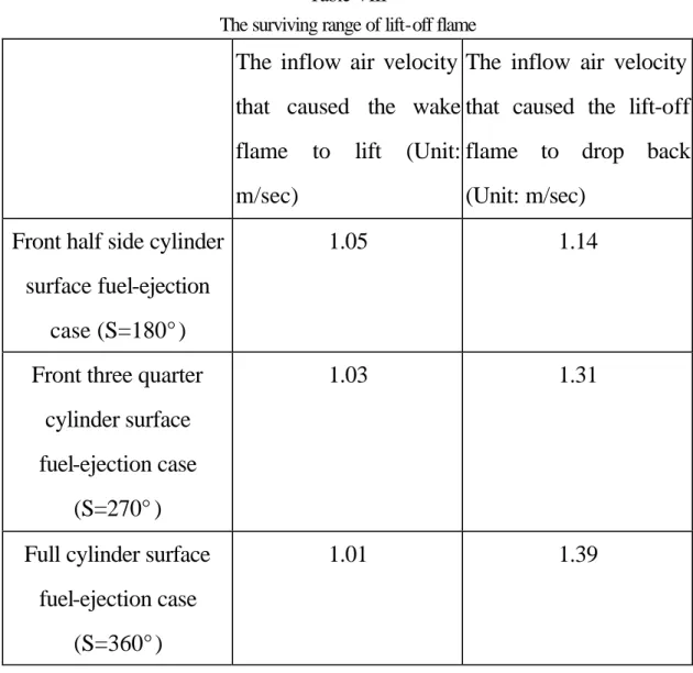
TABLE VIII THE SURVIVING RANGE OF LIFT-OFF FLAME...65

TABLE IX FLAME LIFT-OFF HEIGHT AT VARIOUS FUEL-EJECTION AREA (UIN=1.05 M/SEC) ...66

TABLE X THE CHARACTERISTICS OF EACH KIND OF FLAME FOR S=180° ...67

TABLE XI THE CHARACTERISTICS OF EACH KIND OF FLAME FOR S=360°...69

(9)

LIST OF FIGURES

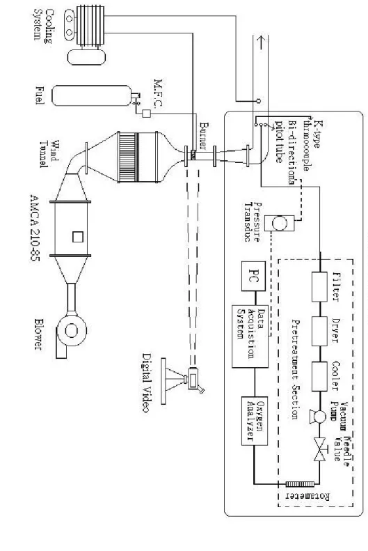
FIGURE 1. SCHEMATIC DRAWING OF OVERALL EXPERIMENTAL SYSTEM ...71

FIGURE 2 BOUNDARY CONDITIONS OF THE PHYSICAL DOMAIN ...72

FIGURE 3 SCHEMA OF THE WIND T UNNEL ...73

FIGURE 4 THE PICTURE OF AMCA 210-85 STANDARD IN W IND TUNNEL...74

FIGURE 5 THE DESIGN FIGURE OF AMCA 210-85 STANDARD...75

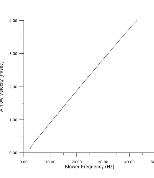
FIGURE 6 THE RELATION FIGURE OF BLOWER FREQUENCY AND AIRFLOW VELOCITY 76 FIGURE 7 THE CONNECTING OF BLOWER AND TUNNEL ...77

FIGURE 8 THE PICTURE OF COOLING SYSTEM ...77

FIGURE 9 THE PITOT TUBE IN TEST SECTION...78

FIGURE 10 THE POSITION OF PITOT TUBE IN TEST SECTION ...78

FIGURE 11 PRESSURE DIFFERENCE AT DIFFERENT POSITION IN TEST SECTION ...79

FIGURE 12 POROUS SINTERED STAINLESS STEEL CYLINDER ...80

FIGURE 13 THE PICTURE OF BURNER...80

FIGURE 14 CYLINDRICAL BRASS ROD ...80

FIGURE 15 THE DIGITAL MASS FLOW CONTROLLER...81

FIGURE 16 THE DESIGN FIGURE OF BI-DIRECTIONAL PITOT TUBE...82

FIGURE 17 THE PICTURE OF BI-DIRECTIONAL PITOT TUBE...82

FIGURE 18 THE PICTURE OF O2 ANALYZER ...82

FIGURE 19 THE CONNECTING PATH IN THE PRETREATMENT SYSTEM ...83

FIGURE 20 THE PICTURE OF THE PRETREATMENT SYSTEM ...84

FIGURE 21 THE MEASURING PROBES IN THE VENT ...84

FIGURE 22 SCHEMA OF INSTRUMENTS BUILDING...85

FIGURE 23 FLAME BLOW-OFF CURVES FOR COUNTERFLOW DIFFUSION FLAME IN THE FORWARD STAGNATION REGION OF A POROUS CYLINDER (R=1.5CM, AND THE FUEL IS METHANE) ...86

FIGURE 24 TEMPERATURE DISTRIBUTIONS THROUGH THE FLAME FRONT OF A TSUJI BURNER WITH R=0.02M, UIN=0.15M/SEC, AND -FW=0.318. THE SOLID LINE AND ITS CORRESPONDING SQUARES ARE THE CARS MEASUREMENTS OF DREIER ET AL. (1986), THE DASH-DOT-DOT LINE AND ITS CORRESPONDING TRIANGLES ARE THE NUMERICAL RESULTS OF DREIER ET AL. (1986), AND THE DASHED LINE AND ITS CORRESPONDING CIRCLES ARE THE NUMERICAL RESULTS OF THE CURRENT STUDY. ...87

FIGURE 25 SERIES OF TEMPERATURE CONTOURS AND STREAMLINES ...89

FIGURE 26 SERIES OF METHANE (SOLID LINES) AND OXYGEN (DASHED LINES) MASS FRACTION CONTOURS ...92

(10)

FIGURE 28 THE MASS FRACTION CONTOURS OF HYDROGEN F OR CASE B4 ...95 FIGURE 29 THE FLAME CONFIGURATIONS FOR THE EXPERIMENTAL VISUALIZATION

(-FW=0.201) ...96

FIGURE 30 SERIES OF TEMPERATURE CONTOURS AND STREAMLINES IN THE FRONT THREE QUARTER SIDE CYLINDER SURFACE FUEL-EJECTION CONDITION (S=270°)

...97 FIGURE 31 SERIES OF TEMPERATURE CONTOURS AND STREAMLINES IN THE FULL

CYLINDER SURFACE FUEL-EJECTION CONDITION (S=360°)...98 FIGURE 32 DEFINITIONS OF FLAME STAND-OFF DISTANCE, FLAME THICKNESS, FLA ME

ATTACHED ANGLE, FLAME LENGTH, AND FLAME LIFT-OFF HEIGHT FOR EACH

KIND OF FLAME ...99 FIGURE 33 VARIOUS FLAME STABILIZATION REGIONS OVER A BURNER (S=180°)...100 FIGURE 34 SERIES OF FLAME CONFIGURATIONS AS A FUNCTION OF INFLOW VELOCITY

(VW = 1.12CM/S AND S = 180°), (A) UIN = 0.41M/S, (B) UIN = 0.51M/S, (C) UIN = 0.66M/S,

(D) UIN = 1.00M/S, AND (E) UIN = 2.06 M/S ...101

FIGURE 35 SERIES OF FLAME CONFIGURATIONS AS A FUNCTION OF INFLOW VELOCITY (VW = 1.23CM/S AND S = 180°), (A) UIN = 0.41M/S, (B) UIN = 0.62M/S, (C) UIN = 0.76M/S,

(D) UIN = 0.89M/S, (E) UIN = 1.04 M/S, (F) UIN = 1.28M/S, AND (G) UIN = 2.35M/S ...102

FIGURE 36 SERIES OF FLAME CONFIGURATIONS AS A FUNCTION OF INFLOW VELOCITY (VW = 2.46CM/S AND S=180°), (A) UIN = 0.41M/S, (B) UIN = 1.00M/S, (C) UIN = 1.2M/S, (D)

UIN = 1.25M/S, (E) UIN = 1.58M/S, AND (F) UIN = 3.10M/S ...103

FIGURE 37 SERIES OF FLAME CONFIGURATIONS AS A FUNCTION OF INFLOW VELOCITY (VW = 3.02CM/S AND S = 180°), (A) UIN = 0.41M/S, (B) UIN = 0.62M/S, (C) UIN = 0.71M/S,

(D) UIN = 1.00M/S, (E) UIN = 1.39M/S (NIGHT SHOT PHOTOS), (F) UIN = 1.43M/S, AND (G)

UIN = 3.00M/S...105

FIGURE 38 VARIOUS FLAME STABILIZATION REGIONS OVER A BURNER (S=360°)...106 FIGURE 39 SERIES OF FLAME CONFIGURATIONS AS A FUNCTION OF INFLOW VELOCITY

(VW = 1.23CM/S AND S=360°), (A) UIN = 0.41M/S, (B) UIN = 0.51M/S, (C) UIN = 0.80M/S, (D)

UIN = 1.00M/S, (E) UIN = 1.05M/S (NIGHT SHOT PHOTOS), (F) UIN = 1.21M/S AND, (G)

UIN = 1.63M/S...108

FIGURE 40 SERIES OF FLAME CONFIGURATIONS AS A FUNCTION OF INFLOW VELOCITY (VW = 1.4CM/S AND S=360°), (A) UIN = 0.41M/S, (B) UIN = 0.51M/S, (C) UIN = 0.84M/S, (D)

UIN = 1.06M/S (NIGHT SHOT PHOTO), (E) UIN = 1.24M/S (NIGHT SHOT PHOTO), AND (F)

UIN = 1.63M/S...109

FIGURE 41 THE TRANSIENT OSCILLATION PHOTOS OF LIFT-OFF FLAME IN UIN =

1.03M/SEC AND VW = 1.12CM/SEC (THE NUMBER 1, 2, 3, AND 4 REPRESENT THE

TIME SEQUENCE.) (LEFT PHOTOS ARE NORMAL ONES AND RIGHT PHOTOS ARE

NIGHT SHOT ONES.) ...110 FIGURE 42 THE PREDICTED TEMPERATURE CONTOURS OF TRANSIENT LIFT-OFF FLA ME

(11)

(12)

NOMENCLATURE

A Cross-sectional area of the test section ABurner Surface area of the half cylinder

a Length of cross-sectional area of the test section B Frequency factor for gas phase reaction

b Width of the cross-sectional area of the test section

C Mole fraction

p

C Mean specific heat at constant pressure

D Cylinder diameter

Di Inner diameter of the cylinder

Do Outer diameter of the cylinder

D Dimensional species diffusivity Da Damkohler number

E Activation energy

-f Nondimensional fuel-ejection rate _w H Flame lift-off height

h Enthalpy

ks Flame stretch rate

K Equilibrium constant k Rate constant

Lc Length of the cylinder

Le Lewis number, α D M Molecular weight

Mair Air molecular weight at STP condition

MT Third-body

N Number of chemical species P Pressure

Pr Prandtl number, ν α Qair Flux of the air

Qfuel Flux of the fuel

R Cylinder radius

0

R Universal gas constant Re Reynolds number S Fuel-ejection area

T Temperature

(13)

w

T Nondimensional wall temperature

*

T Reference temperature t Time

Uin Inflow (air) velocity

u Velocity in x-direction

V Diffusion velocity

v Velocity in y-direction

w

v Fuel ejection velocity on cylinder surface x Distance in x-direction

Y Mass fraction of species y Distance in y-direction z Third-body efficiency Greek * α Thermal diffusivity at T * ì Dynamic viscosity * µ Dynamic viscosity at * T ñ Density * ρ _{Density at} * T air ρ Density of air i

ω& Reaction rate

ν Kinematic viscosity ë Thermal conductivity ë* Thermal conductivity at T* Overhead Dimensional quantities Superscript * Reference state Subscript CH4 Fuel O2 Oxidizer H2O Water vapor CO2 Carbon dioxide CO Carbon monoxide N2 Nitrogen

(14)

H2 Hydrogen

H Hydrogen radical

w Surface of the porous cylinder a Ambient

rc Reference

n, t Normal and tangential to cylinder surface

(15)

CHAPTER 1 INTRODUCTION

1.1 Motivation

This work is motivated by the findings on the appearance of a lift-off flame over a Tsuji burner within a certain range of incoming flow velocity in the recent experimental works of Wang (1998). He concentrated mainly on elucidating the flame structures as a function of distance between a pair of Tsuji burners (dual porous cylindrical burners). To the author’s best knowledge, this is the only experiment in which a lift-off flame was observed over a porous cylindrical burner. Although Gollahalli and Brzustowski’s experiments (1973) also determined a lift-off flame, the burner was a porous sphere rather than a cylindrical one. Chen (1993), Jiang et al. (1995), Huang (1995), Chiu and Huang (1996), and Huang and Chiu (1997) numerically addressed droplet gasification and combustion problems in a forced convection environment. All of them identified the flame lift-off phenomena above a fuel droplet. These phenomena suggest the possibility of a lift-off flame’s existing over a Tsuji burner.

The two-dimensional combustion model developed by Chen and Weng (1990) simulates the stabilization and extinction of a flame over a porous cylindrical burner. Their model employs the one-step overall chemical reaction mechanism. According to their results, the envelope, side, and wake flames appear in order, as the incoming flow velocity was gradually increased. When a limiting value is reached, the flame is completely blown-off from the porous cylinder without the appearance of any lift-off flame. Apparently, this prediction contradicts the

(16)

experimental observation of Wang (1998), mentioned previously, perhaps because of simplified combustion chemistry. Therefore, this study presents a multi-step chemical reaction mechanism to incorporate the original combustion model and further examine the corresponding flame behaviors over a Tsuji burner. Besides, a corresponding experimental set-up, shown in Fig. 1, is built to investigate the counterflow flame behaviors over a Tsuji burner and thereby duplicate the appearance of the lift-off flame. To compromise with the complexity of multi-dimensional and irregular flow field, a four-step methane oxidation chemical kinetics (Paczko et al. [1986], Peters and Kee [1987], Seshadri and Peters [1990], and Rogg [1991 and 1993]) is adopted here without loss of the important role of the chemistry in this reacting flow.

1.2 Literature Survey

Tsuji and Yamaoka (1967, 1969, and 1971) and Tsuji (1982) conducted a series of experiments on the counterflow diffusion flame in the forward stagnation region of a porous cylinder. The corresponding extinction limits, aerodynamic effects as well as temperature and stable-species-concentration fields of this flame were studied in detail. They identified two flame extinction limits. The blow-off, caused by a large velocity gradient (flame stretch), occurs because of chemical limits on the combustion rate in the flame zone. Substantial heat losses cause thermal quenching at a low fuel-ejection rate. However, no lift-off flame phenomenon was reported.

The primary configuration in Chen and Weng’s numerical study (1990) included a flame over a porous cylinder. That study used the two

(17)

dimensional, complete Navier-Stokes momentum, energy, and species equations with one-step finite-rate chemical kinetics. Their parametric studies were based on the Damkohler number (Da), a function of flow

velocity, and the dimensionless fuel-ejection rate (-fw), respectively. As

Da was decreased, the envelope, side, and wake flames appeared in order.

However, reducing -fw caused the envelope flame to directly become a

wake flame, and no side flame was observed.

Sung et al. (1995) utilized a non-intrusive laser-based technique to elucidate the extinction of a laminar diffusion flame over a Tsuji burner. A laminar diffusion flame, unlike a premixed flame, is sensitive to variation in the imposed strain rate. It becomes thinner with an increasing rate, leading to an increase of reactant leakage, progressively reducing flame temperature, and eventually causing extinction of laminar diffusion flame. Zhao et al. (1997) utilized USED CARS to measure the temperature distribution in the forward stagnation and wake regions of a methane/air counterflow diffusion flame. A pyrolysis zone of methane is observed on the fuel-rich side of the stagnation region. The temperature of the flame in the wake region was found to exceed that in the stagnation region, implying that some intermediate products were not completely burnt in the latter region.

Considerable progress has been made during the preceding two decades in predicting the structure of steady counterflow diffusion flames using complicated mechanisms of reaction. The GAMM at Heidelberg was the most famous workshop, and it included five different groups. Dixon-Lewis et al. (1984) used one-dimensional complex chemical

(18)

reaction mechanisms, with detailed transport properties, to predict the structure of the counterflow diffusion flame in the front stagnation region of a Tsuji burner. Their computed results did not fully match Tsuji and Yamaoka’s measurements (1971). They claimed that the reason for the discrepancies was the overall system’s failing to behave as a straightforward boundary layer flow, and that a full solution requires a two-dimensional flow treatment.

Dreier et al. (1986) and Sick et al. (1990) made CARS measurements and one-dimensional calculations to elucidate the counterflow diffusion flame over a porous cylinder. Their chemical reaction mechanism involved 250 elementary steps (including reverse reactions) and 39 species. As in the last reference, they found that discrepancies between experimental and computational results followed from applying boundary layer approximations. Apparently, the flow field must be completely represented in two dimensions.

Wohl et al. (1949) stated that, as the burning velocity of the premixed flame equals the speed of the local fluid at which the laminar flame velocity is maximum, the diffusion flame can be lifted. Vanquickenborne and Van Tiggelen (1966) developed this idea further. This theory is fundamentally based on complete molecular-scale mixing, which occurred in the unburnt flow upstream from the flame stabilization point. Kalghatgi (1984) introduced the following relationship to explain the occurrence of lift-off flames.

5 . 1 max , max , 50 _          = ∞ ρ ρ ν µ ρ _e L e e L e S h S ,

(19)

where SL, max is the maximum laminar flame velocity, occurring near stoichiometric conditions for hydrocarbons. The flame structure in the stabilization region was fuel/air fully premixed.

1.3 Scope of the Present Study

This study modifies the combustion model of Chen and Weng (1990). The modification involves adopting a four-step chemical reaction mechanism and a finer distribution of grid size to catch up the flame lift-off phenomena over a Tsuji burner immersed in a uniform air stream by ejecting methane uniformly from the surface of a cylinder. Besides, this work sets up an apparatus for duplicating the lift-off flames and examines the appearances of the flames. The main configuration is similar to that employed in the experiments of Tsuji and Yamaoka (1967, 1969, and 1971). The parameters of interest are the inflow air velocity

(Uin) and fuel-ejection area (S) of the cylindrical burner. This work

aims to determine under which condit ions the lift-off flame can exist, and then to analyze the detail of the structure of such a flame. A physical interpretation is presented to clarify the mechanisms of the flame’s lifting and dropping back. This work also involves flow visualization of the flame behaviors recorded by a digital video. These data are directly compared with the corresponding numerical simulation, and vice versa.

(20)

CHAPTER 2 MATHEMATICAL MODEL

The proposed mathematical model, including assumptions, normalization procedure, and the corresponding solution methodology, including a grid generation technique and algorithm, are similar to those developed by Chen and Weng (1990). The major improvements are that the chemical kinetics adopts a four-step mechanism rather than a one-step mechanism, and the grid cell is much smaller due to the current availability of far superior computational tools. Consequently, this section emphasizes the description of the four-step chemical kinetics mechanism, the corresponding formulae and boundary conditions.

2.1 Nondimensional Conservation Equations

Table I summarizes the nondimensional continuity, x-momentum, y-momentum, and energy conservation equations used in this work. For the details of the normalization procedure, please refer to Chen and Weng (1990). The dimensional energy and species equations and the representations of corresponding properties are as follows.

Energy equation

∑

= −             +     = + N i i i p p h C T y C T 1 1 y x T x 1 y v x T u ω ∂ ∂ λ ∂ ∂ ∂ ∂ λ ∂ ∂ ∂ ∂ ρ ∂ ∂ ρ & (1) Species equation i i i i i i i _D y D ω ∂ ∂ ρ ∂ ∂ ∂ ∂ ρ ∂ ∂ ∂ ∂ ρ ∂ ∂ ρ _+ &      +     = + y Y x Y x y Y v x Y u , i=1, 2…, N-1 (2)

where i represents CH4, O2, CO2, H2O, CO, H2, and H, and the mass

(21)

∑

− = − = 1 1 1 2 N i i N Y Y (3)

The equation of state of an ideal gas is used to close Eqs. (1) and (2):

∑

₌ ° = N i i i M Y T R P 1 ρ (4)

The above equation is rewritten to express ρ as,

∑

= ° = _N i i i M Y T R P 1 ρ (5)

Rogg’s approximation (1993) is adopted to express the diffusion flux:

x Y Le C x Y D i i p i i ∂ ∂ = ∂ ∂ λ ρ (6)

The Lewis numbers used in this numerical calculation are (Seshadri and Peters [1990] and Bilger et al. [1991]),

97 . 0 4 = CH Le , LeO₂=1.11, LeH2O=0.83, LeCO2=1.39, 2 H Le =0.3, LeH =0.18, LeCO=1.1, LeN2=1.0 (7)

A new correlation is introduced to express

p

C λ

in Eq. (6) (Seshadri and Peters [1990] and Rogg [1991]).

7 . 0 5 298 10 58 . 2       × = − T Cp λ (8)

The mean specific heat at constant pressure, Cp, can be written as (Kee

et al., 1999A),

∑

= = N i i p p C Y C i 1 (9) NASA thermochemical polynomials (Andrews and Biblarz [1981] and

Kee et al. [1999B]) are used to estimate the specific enthalpy, hi, and the

(22)

4 , 5 3 , 4 2 , 3 , 2 , 1 a T a T a T a T a Cpi = _i + _i + _i + _i + _i (10) i i i i i i i T a a T a T a T a T a h ₁_, 2, 2 3, 3 4, 4 5, 5 ₆_, 5 4 3 2 + + + + + = (11)

The Prandtl number is defined as,

p p C C λ µ λ µ ₌ = Pr (12)

Thus, the dynamic viscosity can be expressed as,

p

C λ

µ= Pr× (13)

In this work, Pr = 0.75 is selected following Smooke and Giovangigli (1991), and Eq. (8) is introduced as follows.

7 . 0 5 298 10 58 . 2 75 . 0 _      × × = − T µ (14)

The dynamic viscosity can thus be expressed as,

7 . 0 7 10 586985197 . 3 × ×T = − µ (15) 2.2 Chemical Kinetics

The four-step chemical reaction mechanism used in this study is

reduced from a 58-step C1 mechanism that was used by Miller et al.

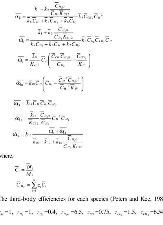
(1984). The four-step reaction (Paczko et al. [1986], Peters and Kee [1987], and Rogg [1993]), involving seven reacting species and nitrogen, are presented below.

CH4+H2O+2H CO+4H2 (I)

CO+H2O CO2+H2 (II)

2H+MT H2+MT (III)

(23)

The mass production rate for each species (Rogg, 1991) can be expressed as, I CH CH M ω ω& ₄ & 4 =− (16) IV O O M ω ω& ₂ & 2 =− (17) II CO CO M ω ω& ₂ & 2 = (18)

(

I II IV

)

O H O H M ω ω ω

ω& ₂ = − 2 & + & − 2& (19)

(

I II

)

CO

CO M ω ω

ω& = & − & (20)

(

I II III IV

)

H

H M ω ω ω ω

ω& ₂ = 2 4 & + & + & − 3& (21)

(

I III IV

)

H

H M ω ω ω

ω& = − 2& +2 & − 2 & (22)

0 2 = N

ω& ₍₂₃₎

The rates of reactions (I)∼(IV) (Peters and Kee, 1987) are derived as follows.

2

1 ω

ω

ω&_I ₌ & ₊ & (24)

9 ω ω&_II ₌ & (25) 15 14 8 6 ω ω ω ω

ω&_III ₌ & ₊ & ₊ & ₊ & (26)

16

10 ω

ω

ω&_IV ₌ & ₊ & (27)

in which ω&1 , ω&2 , ω&6 , ω&8 , ω&9 , ω&10 , ω&14 , ω&15 , and ω&16 can be

obtained from Peters and Kee (1987):

H CH C C k1 4 1 = ω& (28) H CH H O H C C C C C K k 4 2 2 12 2 2 = ω& (29)

(24)

2 6 8 7 6 12 2 1 6 4 2 2 2 H CH O M H C H O H C C k C k C k C k K C C k k T + + + = ω& (30) H CH O M H O C H O H C C C k C k C k C k K C C k k T 4 2 2 2 2 8 7 6 8 12 2 1 8 + + + = ω& (31)       − = II CO H O H CO H C K C C C C C K k 2 2 2 12 9 9 ω& (32)     ₋ = IV H O H H O H K C C C C C k ₃ 2 2 10 10 2 2 2 ω& (33) T M O HC C C k14 2 14 = ω& (34) T M H H O H C C C C C K k 2 12 15 15 2 2 = ω& (35) 12 18 17 16 14 8 16 16 2 2 C H O H K C C k k k k + + + = ω ω

ω& & & ₍₃₆₎

where, i i i M Y C = ρ (37)

∑

= = N i i i M z C C _T 1 (38) The third-body efficiencies for each species (Peters and Kee, 1987) are

H

z =1, zH₂ =1, zO2 =0.4, zH2O=6.5, zCO=0.75, zCO2=1.5, zCH4=6.54, and

2

N

z =0.4.

Table II (Warnatz, 1984) shows the rate constants used in Eqs. (28-36). However, some equilibrium constants, such as those in Eqs. 29-33, 35, and 36, are using the ones proposed by Peters and Kee (1987).

      ° = − T R T KC 15130 exp 2657 . 0 0.0247 12 (39)       ° × = − T R T KII 9839 exp 10 828 . 3 5 0.8139 ₍₄₀₎

(25)

      ° = − T R T KIV 11.687 exp 11396 2467 . 0 (41)

Finally, all ω&is are divided by

R U_in

*

ρ

to yield the nondimensional

value, ω&i, for each species.

2.3 Nondimensional Boundary Conditions

The domain of interest can be reduced to a half plane because the two-dimensional flame is assumed to be symmetric with respect to the

stagnation streamline ( y =0 ), and Fig. 2 illustrates the boundary

conditions.

The surface temperature of the cylindrical burner is maintained constant. The fuel is uniformly ejected from the front half surface of the porous cylinder. Thus, the boundary conditions along the surface are,

t

v =0, v_n=−f_w(2/Re)0.5, T_w=given, m& _w = v_nρ_w (42)

w f w fw w n Y Le Pr Re 1 m Y m ∂ ∂ µ + = & & (43) w o ow w n Y Le Pr Re 1 Y m ∂ ∂ µ = & (44) w o i iw w n Y Le Y m ∂ ∂ = µ Pr Re 1 & , (45)

where i=CO2, H2O, H2, N2, H, and CO. If the surface is non-blowing,

then the boundary conditions become,

t v =0, v_n=0, T_w=given, m& _w=0 (46) w f n Y ∂ ∂ =0, o _w n Y ∂ ∂ =0, i _w n Y ∂ ∂ _{=0 (47)}

(26)

2.4 Numerical Algorithm

The configuration of the flow field, as depicted in Fig. 2, is irregular. Therefore, a body-fitted coordinate system, generated by a grid generation approach, is employed. Accordingly, the physical domain is transformed into a computational domain that consists of the equally spaced, square grids. Weng (1989) detailed the procedure, which is not presented here.

The computational domain is selected to be xin = -7, xout = 13, and

ywall = 4. The upstream and downstream positions are determined via

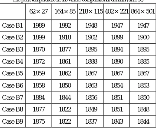
several numerical experiments to meet the requirement that applying boundary conditions at these positions sho uld not impact the flame structures. Then, a set of numerical tests is conducted to ensure further that the resultant solutions are grid-independent. Table III presents test results. The cases shown in the first column are the same as those in Fig. 25, which will be discussed later. If the number of cells exceeds 218×115, then the variation of resultant peak temperature, the variable most sensitive to the size of the grid, over the entire computational domain becomes insignificant by the increasing number of grid cells. Therefore, this work uses 218x115 grid cells. The grid is much finer than that, 112×51, used in the earlier study (Chen and Weng, 1990).

(27)

CHAPTER 3 Experimental Apparatus Setup

Basically the experimental setup is incorporated with the present combustion model. The experimental setup consists of three major elements in the apparatus, which are the wind tunnel, the porous sintered cylindrical burner and measurement instrumentations. They are described in detail as follows.

3.1 Wind Tunnel

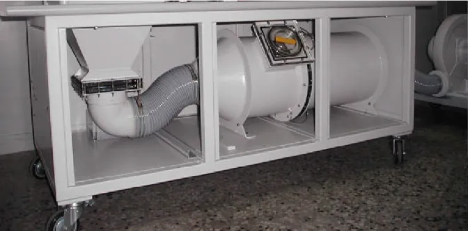
According to the simulation, the tunnel is used to provide a laminar, uniform oxidizer flow to the porous cylindrical burner, and the fuel is injected from the surface of the burner. It is open-circuit and oriented vertically upwards. A schematic configuration of the wind tunnel is shown in Fig. 3. There are five components in the wind tunnel: (1) a blower, (2) a diffuser, (3) flow straightener, (4) a contraction, and (5) a test section. Concepts of making wind tunnel mainly are from Yang et al. (1999).

3.1.1 Blower

The airflow in the tunnel is provided by a variable-speed (frequency controlled) blower (Type TB-201, C-F Company), whose outlet is connected to the main part of the wind tunnel via a flexible 60 cm long and 10 cm diameter plastic ductwork, which the end is coupled to a diameter 346 mm and 75 cm long cylinder, which is designed according as AMCA 210-85 standard (shown in Figs. 4 and 5). The blower is driven by a frame motor, which is controlled by an inverter drive. A

(28)

frequency converter (Type M36V2P07, DYNAGEN, J-C Company) is used to control the rotational speed of blower to get the desired velocity. The frequency of the blower and corresponding velocity in test section shown in Fig. 6. In order to avoid the influence of vibration, the base of wind tunnel and blower are separated (shown in Fig. 7).

3.1.2 Diffuser

A 30 cm long diffuser has an inlet cross-section area of 12x12 cm2

and the outlet one is 40x40 cm2. The expansion ratio based on area is

1:11.

3.1.3 Flow Straightener

The airflow from diffuser section is really unstable before entering into contraction section. The flow straightener is used to make it more stable. The flow straightener section, which serves to insure that the flow to test section is laminar and uniform over the entire cross-section, consists of honeycomb and screen. The screen is mounted to decrease disturbances and make flow uniform. The honeycomb is added to utilities of the screen, like reducing turbulence effect. With appropriate combinations of screen and honeycomb characteristics and putting them at optimum position, it can achieve the goals mentioned above.

3.1.4 Contraction Section

The test section cross-section area 24x4 cm2, therefore the

contraction ratio over the contraction section is 16.6:1. Its purpose is to promote a uniform field in the test section. The design criteria are

(29)

demanded to shorten the duct and reduce boundary layer thickness along the wall as possible.

3.1.5 Test Section

The test section has a cross section area of 24x4 cm2 and a length of

30 cm. It is made up four sides. In the front and two connecting sides, they are equipped with quartz-glass plates for observation windows. The rear side is made of stainless steel plate for supporting the burner to insert. The downstream of the test section is connected to a diffuser (500 mm), which can reduce the amount of exhaust gases from test section. The vent follows after the diffuser to outdoor. The rear part of the vent can resist high temperature by adhered fins to inside the vent as heat exchanger. The outside of vent is connected with water-cooling system, including cooler, water tank and pump (shown in Fig. 8). The front part of inside the vent is also very important since a series of instruments are set up to measure the heat release rate (see Sec. 3.3.6).

Measurement in the test section is to confirm the velocity uniform and stable. There are four sets of pitot tubes and a fixed static pressure hole in the front of the burner of the test section (see Figs. 9 and 10). Change different connection in four pitot tubes in order (fixed the static pressure hole) under the same inflow velocity after a long time. If the pressure difference is closely equal, it means that the flow is uniformity and stabilization (see Fig. 11).

3.2 Porous Sintered Cylindrical Burner

(30)

The requirement of experimental burner has to be able to sustain the high temperature. It is designed to have inner and outer parts, respectively. The outer part of burner is a replaceable porous sintered stainless steel (20, 40, 70μm pores, respectively) with a length of 40± 0.5 mm. Its inner diameter is 20±0.5 mm, and an outer diameter 30± 0.5 mm (see Figs. 12 and 13). The advantage of this design is that the burner replacement can be easily performed whenever clogging or damage on the porous burner surface occurs due to burning for a long time. The inner of the burner is a cylindrical brass rod (see Fig. 14) with an internal water-cooling groove and fuel supply groove. The outer part is screwed on the inner part. The internal water flow is used to cool the burner to prevent damage from the porous surface structure. The cooling device of the burner includes a water tank, pump, cooler and connected-piping (shown in Fig. 8).

3.2.2 Burner Equipped to Test Section

There are two parameters (half fuel-ejection surface and full fuel-ejection surface respectively) to be measured. Therefore, for the front half side cylinder surface fuel-ejection condition, coating several thin layers of high temperature resistant paint on the backward portion of the burner surface in order to prevent the fuel ejection into the wake region.

(1) The painted surface needs to dry at least 2 hours.

(2) Screwing the burner into the insert and mounting the burner closely to the wall of test section. Connecting the cooling water and fuel pipelines to the burner.

(31)

(3) Noticing to adjust the burner so that the uncoated burner surface is facing the direction of the airflow.

(4) In addition, it’s important to test whether there is any leakage from the painting surface of the burner. Instead of fuel pipe to air or nitrogen piping, and then immerse the burner into a water container and open a valve to let gas flow to observe whether there are bubbles from the painted surface.

Methane (CH4, 99.99%) is used as the fuel, and its flow is controlled

and measured by a flow meter. A digital mass flow controller (Type MC-2100E, LINTEC, shown in Fig. 15) is controlled by high capability of microprocessor inside. The sensor flow rate signals and command signals are digitized by 16 bit A/D converter to process and operate inside CPU (including: temperature compensation, linearity compensation and control signals operations), and then transformed flow rate signals and command signals into analog signals by 16 bit D/A converter. The fuel ejection velocity is calculated by dividing the fuel volumetric flow by the available fuel ejection area of the burner surface.

3.3 Measurement Instrumentations

3.3.1 Nozzle of the AMCA 210-85 Standard

The measurement of inlet velocity at the test section adopts the AMCA 210-85 standard of nozzle-method to measure volume flow rate and then to deduce flow velocity. The standard is adopted to establish uniform methods for laboratory testing of fans and other air moving devices by AMCA (Air Movement & Control Association Inc.). There

(32)

are three nozzles (Ö: 10, 15, and 30 mm) and four sets of pitot tubes distributed equally inside the cylinder (shown in Fig. 5), which are incorporated to measure local velocity of the cylinder. Then it can get total volume flow rate to deduce velocity of test section by dividing cross section area of test section. The precision is within 3% when velocities are ranged from 0.21 m/sec to 3.3m/sec precision, but it becomes 5% as the velocity is smaller than 0.21 m/sec.

3.3.2 Digital Video

A digital video (Type DCR-TRV17, SONY) is used to record the flame profiles, such as envelope, side, wake flame, and flame lift-off. It is fixed on appropriate position to catch flame variations. The special function applied is night-shoot to record various flames in the dark laboratory. All imagines recorded on the tape of the cassette have to transmit to computer to process. The digital video is connected to computer by IEEE 1394 card, and then imagines processed by Ulead Video Studio software to show a series of flame structures in different velocity regime.

3.3.3 Thermocouples

K-type thermocouple (wire diameter, 1 mm; compensation wire diameter, 0.65 mm) is used to measure the temperature in order to get the corresponding density in the exhausted duct. It is made of Ni-Cr/Al-Ni alloy material, compensation time 1 second and measured temperature up to 1200 ℃. The measured signals are connected to data acquisition device (PC Recorder, M-SYSTEM) to transform analog signals into

(33)

digital signals by series port RS-232 to computer with MSRS32-E software.

3.3.4 Pressure Transducer

Pressure drop received from bi-directional pitot tube (see Figs. 16 and 17) in the vent is converted into micro-voltage signal by pressure transducer. Via this procedure, the averaged velocity in the duct can be calculated. And pitot tubes in the test section and in front of the nozzles of the cylinder are also measured by the pressure transducer (Type PF-MPS2, POUNDFUL).

3.3.5 Oxygen Analyzer and Pretreatment System

Oxygen analyzer (Mode 755A O2 Analyzer, shown in Fig. 18) is

used to measure oxygen consumption in the vent. It should be calibrated and zeroed before testing, using 99.99% pure nitrogen as the zero gas and the air as the span gas, which is composed of 21% oxygen and 79% nitrogen (all gases produced by J-R Gas Company). Exhausted gas should be filtered and cooled completely in the pretreatment section to avoid high temperature and other suspended grains to damage the analyzer. It may reduce oxygen concentration and result data unstable. The pretreatment system is constructed of two sets of series glass wool filter, a membrane filter, and a cooler and micro pump to introduce gas inlet (shown in Fig. 19). The whole schematic piping arrangement of pretreatment system is shown in Fig. 20. The measured signals are connected to data acquisition device (PC Recorder, M-SYSTEM) to

(34)

transform analog signals into digital signals by series port RS-232 to computer with MSRS32-E software.

3.3.6 Heat Release Rate Measurements

The flame strength is quantified by the heat release rate. Such measurement is carried out in the exhausted duct, which includes: (1) K-type thermocouple, (2) a robust bi-directional probe connected to pressure transducer and (3) a gas sampling probe connected to the oxygen analyzer with the pretreatment section (shown in Fig. 21). These instruments are used to measure the temperature, velocity and oxygen concentration of oxygen of product gas, respectively. All the sampling gases are first introduced to the pretreatment section for cooling and filtering before they go into the oxygen analyzer. The whole schematic configuration can be seen in Fig. 22. The signals will be collect via a data acquisition system, and then these data are handled by 586-PC to calculate the heat release rate.

3.4 Procedure of the Experimental Operation

(1) Calibrate the instruments to make sure the stabilization and accuracy of their performance before performing the experiment. (2) It usually takes times for completion of warm-up for the

apparatuses that include blower, mass flow controller and O2

analyzer.

(3) The blower has to be operated for 30 minutes until the flow uniformity and stabilization are achieved. Stabilization depends on pressure difference (four pitot tubes vs. 1 fixed static pressure

(35)

hole) in front of the burner in the test section is stable.

(4) The digital mass flow controller needs to be operated for 15-30 minutes because of thermal-sensor type to let flow more accurate.

(5) Check if any fuel gases leak from pipelines by suds. It’s very important procedure for this achromatic, flavorless, toxic and flammable fuel.

(6) Turn on the flow of cooling system to the burner and vent.

(7) Start the computer program (software: MSRS32-E) used to collect desired data via a data acquisition system (PC Recorder), and then these data are handled by 586-PC using software to calculate the heat release rate.

(8) Turn on the ignition device, which is produced spark by the way of 3000 volt high voltage. Turn it off until the flame is established. Note that remember to ignite first before let the fuel input, or it may be exploded.

(9) Open the valve of methane fuel vase and keep inlet pressure up to 8 psi, then turn on the stop valve of mass flow controller. The alarm light of mass flow controller displays green that means fuel passes pipelines to the burner. Set the fuel flow rate to the desired amount in liters per minutes. First choose a certain fixed value of fuel supply to the burner, and then increase slowly the airflow velocity in order to get various flame types. It means that change the inflow velocity as a parameter under a fixed fuel ejection rate.

(36)

appear. Once the flame is established, permit several minutes for the flame to stabilize or adjust the blower speed if necessary. Next, gradually increase the inflow velocity to get the other types of flames. After that, change another value of fixed fuel ejection rate to continue this step. Then it can gain profiles of different fuel flow rate as increasing inflow velocity.

(11) Digital video is fixed to position to get the same observation view of test section to catch all images from testing.

(12) Using the front half side fuel-ejection of cylinder surface instead of full side fuel-ejection burner to repeat the procedure from (8)-(10) steps.

(13) Also change the fuel ejection rate as a parameter under a fixed flow velocity. Carry out the similar procedure as the above.

3.5 Uncertainty Level Analysis in the Experiment

Uncertainty analysis is carried out to estimate the uncertainty levels in the experiment. Formulae for evaluating the uncertainty levels in the experiment can be found in several papers (Kline and Mcclintock [1953] and Moffat [1982]) and textbooks (Holman [1989], Fox and McDonald [1994], and Figliola and Beasley [1995]). Accordingly, Table IV summarizes the results of all uncertainty analyses.

3.6 Experimental Repeatability

The procedures for changing the airflow velocities at different fuel ejection velocities were performed three times to ensure experimental repeatability, coincidence, and accuracy. The transition velocity, which

(37)

transforms an envelope flame into a wake flame, is a critical value to investigate the flame behaviors. Table V presents the transition velocities for flame transformation from an envelope flame into a wake flame in the front half cylinder fuel-ejection system as a function of fuel ejection velocity. The table records three measured data, their average, and the error at each fuel ejection velocity. The error is defined as the ratio of the absolute difference between the maximum and minimum values of the three data to their average. Generally, the errors are within an acceptable range (maximum of 6.82%) and the repeatability is quite

good except at three points, vw = 1.12 cm/s, 1.23 cm/s, and 1.68 cm/s.

These points are near the two demarcation lines, between region I (vw =

0.9 ~ 1.12 cm/s) and II (vw = 1.23 ~ 1.57 cm/s), and region II and III (vw

= 1.68 ~ 2.8 cm/s). The errors are inevitably large at these critical points. The flame transition processes and their corresponding characteristics are detailed below.

(38)

CHAPTER 4 RESULTS AND DISCUSSION

I. Simulation Part

The gaseous fuel used is methane (CH4) and the ambient oxidizer is

air. The basic thermodynamic and transport property data, summarized in Table VI, are taken from Chen and Weng (1990) to enable a fair comparison later.

4.1 Comparison with Related Experiments and Simulations

The present combustion model is first validated by comparing the predicted results with the pertinent measurements of Tsuji (1982) and the simulation results of Chen and Weng (1990). Then, the predictions are compared with the measurements and calculations of Dreier et al. (1986).

Figure 23 presents the comparison, by plotting the blow-off limit as

functions of -fw (nondimensional fuel ejection rate) and 2Uin/R (flame

stretch rate, ks). Notably, this line in Tsuji’s experiment (1982)

represents a demarcation line at which the flame is transformed from an envelope flame to a wake flame instead of being extinguished. The predictions of this report are quite close to Tsuji’s experiments (1982) in the regions of high fuel-ejection rate and low stretch rate. Generally, the prediction is much better than that of Chen and Weng (1990), implying that the prediction that is based on a four-step chemical mechanism is indeed better than the one that uses a one-step overall chemical

mechanism. However, in the domain of 0.2 < -fw < 0.77 and 91 <

2Uin/R < 376, a significant discrepancy exists between the present

(39)

located at a transition from the very small fuel ejection rate to the large flame stretch rate. The discrepancy may be attributable to two factors stated in Chen and Weng (1990): the first is the three dimensional effect in the experimental configuration and the other one is a chemical effect. The blow-off that results from a low fuel ejection rate is very close to that obtained experimentally because it is governed mainly by the thermal quenching of the cylinder surface. The geometric effect should be minor in this branch. However, aerodynamic and chemical limitations greatly affect the blow-off mechanism due to flame stretch. For a given

2Uin/R (~ 376), in the higher -fw regime (> 0.77), the four-step chemical

effect seems appropriate even if the fluid flow dominates, whereas it does

not suffice to describe the reactions in the regime of lower -fw, such as 0.2

< -fw < 0.77. Better agreement with measurements initiates from -fw =

0.5 and 2Uin/R = 128, which occurs much earlier than that of Chen and

Weng (1990), and continuously improves thereafter.

Figure 24 compares the predictions in this study to the measurements and calculations of Dreier et al. (1986). This figure depicts the temperature distribution along the forward stagnation line, where the forward stagnation point is at x = 0. The presented combustion model reproduces the data measured in the experiment, and the agreement is much better than that of their own numerical computation. The temperature profile on the oxidizer side predicted in this study shifts to the left of the experimental data by around 0.2mm; the shift is approximately 0.5mm on the fuel side. Considering the experimental uncertainties, the agreement can be regarded as excellent.

(40)

Now, Table VII and Fig. 25 directly compare with the results of Chen and Weng’s simulations (1990). Table VII depicts the inflow velocity range for flames with different appearances. Notably, no side flame exists in this study, whereas neither lift-off nor subsequent late wake flames appeared in Chen and Weng (1990). Apparently, the application of a four-step mechanism shows its influence on flame structures. This table reveals that applying a one-step overall chemical reaction can yield a stronger flame if still survives, implying that the corresponding gross reaction rate is higher. However, the velocity range of flame that exists in this work can be sustained to a higher inflow velocity, indicating that the intermediate species generated in the multi-step reactions may play important roles near the extinction limit.

A case in the envelope flame is selected to demonstrate flame structures using different chemical mechanisms, because finding the same type of flame in both cases simultaneously at the same inflow velocity

and blowing rate is difficult; see Table VII. The inflow velocity and -fw

are fixed at 0.75m/sec and 0.5, respectively.

Figures 25-A1 and 25-B1 are the combinations of resultant isotherms and streamlines for Chen and Weng’s (1990) and the present works, respectively. The flame is seen to be smaller and the flame temperature is lower in this study. The maximum temperature is approximately 1860K, but it is about 2300K in the last reference. As mentioned previously, if an envelope flame can exist, the net reaction rate is lower by using a multi-step chemical kinetics.

The streamline patterns in both studies (Figs. 25-A1 and 25-B1) are very similar since the flame, but not chemistry, directly influences fluid

(41)

flow. The recirculation flow region behind the cylinder in Chen and Weng (1990) is smaller than that in this study because the stronger flame in their work generated a higher pressure due to thermal expansion, which depresses the recirculation zone behind the cylinder further.

Figures 26-A1 and 26-B1 present the methane and oxygen mass fraction distributions. Since the reaction rate is slower in this study, the

amount of unreacted fuel (CH4) is expected to be greater, and this fuel

can be carried further downstream by convection and diffusion. Again, this study involves seven reacting species, whereas Chen and Weng (1990) considered only two. Accordingly, the mass fraction of fuel in this work is further diluted since more species are used.

The above three comparisons indicate that the proposed combustion model, which considers a four-step chemical mechanism, can generate a satisfactory solution for the various structures of flames over a single Tsuji burner. The parametric studies are presented below after these comparative works.

4.2 Parametric Studies

The varying parameters are the oxidizer flow velocity (Uin) and the

fuel ejection area (S), respectively, under the specified -fw = 0.5 and R =

1.5 cm. The variation of fuel ejection area (S) is indicated by angle. For example, 180° implies that the fuel ejection area covers the forward half of cylindrical surface, and 360° covers the whole surface.

(42)

Increasing Uin augments the flame stretch rate, ks, defined as 2Uin/R. The inflow velocity varies from 0.75 m/s to 2.12 m/s, and Figs. 25, 26, and 27 are used to illustrate the variations and structures of the corresponding flame. Figure 25 displays a series of combinations of

isotherms and streamline distributions as a function of Uin or ks. Figure

26 presents the combinations of fuel and oxidizer mass fractions, and Fig. 27 plots the fuel reactivity distributions. In Fig. 27, this work adopts the

sec 10 4 ₃ 4 ⋅ = − cm g CH

ω& contour line as a flame boundary, as presented by

Nakabe et. al. (1994).

Figures 25 and 27 show that as the inflow velocity increases, the envelope flame (Fig. 25-B1), wake flame (Figs. 25-B2 and 25-B3), lift-off flame (Figs. 25-B4~B9), and wake flame (Figs. 25-B10 and 25-B11) appear in order before the flame is completely extinguished. Three types of flame exist in the flow field; they are envelope, wake, and lift-off flames. However, the wake flames can be further classified into two categories, transformed from envelope flame or transformed from lift-off flame. Notably, no side flame, which was identified in Chen and Weng (1990), appears in the flow field. This work emphasizes the transition from wake to lift-off and then to wake flame.

4.2.1.1 Envelope Diffusion Flame

An envelope flame surrounds the porous cylinder in the low-speed flow regime. Its velocity is under 0.9m/sec (see Table VII). Case B1 in Fig. 25 belongs to this category.

As shown in Fig. 25-B1, an envelope flame seems to be situated around the front porous cylinder and spreads downstream. The active

(43)

reaction zone in Fig. 27-B1 also exhibits this feature. Such a flame is identified as a diffusion flame, whose fuel side can be distinguished from the oxidizer one, as shown in Fig. 26-B1.

In Fig. 25-B1, the maximum temperature along the stagnation streamline (y=0) is about 1860K at x=-1.455. The isotherms above 600K (indicated by dark blue lines) in front of the burner are almost parallel to the cylindrical surface, because of the uniform fuel-ejection rate. The fact is confirmed by Fig. 27-B1, too. Therefore, the flame stand-off distance can be regarded as constant along the fuel supply surface. This uniform fuel supply, in an opposite direction to the flow of the oxidizer, makes the concentration of isotherms on the oxidizer side denser than that on the fuel side in front of the cylinder. Just behind the fuel supply surface, the isotherms are no longer parallel to the surface but are dispersed. The isotherms on the fuel side shift inward at the back of cylinder and reach the line of symmetry to form a closed loop, since no blowing is applied over there. The recirculation flow in the wake region somewhat distort some intermediate isotherms near the rear stagnation area, such as those of T=900, 1200, and 1500K, as depicted in Fig. 25-B1. The isotherms on the oxidizer side initially move outward, and then spread to the wake. Far downstream, where the influence of the flow recirculation is negligible, the temperature gradient in the cross-stream direction is found to exceed greatly that in the direction of the stream.

4.2.1.2 Wake Flame

Increasing the inflow velocity up to 0.9 m/sec (case B2) breaks the flame front away from the front stagnation streamline. The flame front

(44)

retreats along the surface until a certain condition is met that it can be stabilized on the rear part of the cylinder; see Figs. 25-B2, 25-B3, 27-B2, and 27-B3. This kind of flame is defined as a wake flame. The wake flames in cases B2 and B3 are generated by the break-up of the envelope flame due to the flame stretch effect, as described below. Such a wake flame exists for between 0.9 and 1.04 m/sec; see Table VII. Two other cases, B10 and B11, are also categorized as a wake flame but with a different formation procedure. These will be discussed after the lift-off flame is described.

As shown in Figs. 25-B2, 25-B3, 27-B2, and 27-B3, the wake flame front does not touch the cylinder surface and it is positioned in front of the rear stagnation point; instead, the quenching effect of a cold wall produces a reaction-frozen zone between the flame and the surface. The break-up of the envelope flame in the porous section of the cylinder causes a fuel-air mixture to exist in that region. The mixture is generated from the impingement of fuel and oxidizer streams. Then, the mixture moves downstream by convection, and is ignited by the reversed hot combustion gas products in the vortex region, as shown in Figs. 26-B2 and 26-B3. The location of the flame front is near the top of the recirculation flow. The recirculation flow not only brings hot gases from downstream to upstream to ignite the mixture but also stabilizes the flame. This behavior resembles that of the bluff-body flame holder in afterburner and ramjet systems.

Figures 26-B2 and 26-B3 indicate that the air and fuel are well mixed before entering the reaction zone, since the flame front is away from the porous section and no fuel is ejected from the rear surface. The

(45)

mixture also has time to diffuse to some extent. Consequently, the wake flame front is flat and broadened and presents a premixed flame feature.

4.2.1.3 Lift-off Flame

Unlike that described by Chen and Weng (1990), the wake flame is observed to lift rather than blow-off when the inflow velocity is further increased. When the inflow velocity is raised from 1.04 m/sec (Fig. 25-B3) slightly to 1.05 m/sec (Fig. 25-B4), the wake flame is suddenly transformed into a lift-off flame, which exists between 1.05 and 1.15 m/sec.

Figures 25-B4~B9 indicate that the lift-off flame fronts are not attached to but far from the rear surface of the cylindrical burner. More explicitly, the flame front is behind the rear stagnation point; see Figs. 27-B4~B9. The lift-off height is defined as the stream-wise distance between the rear stagnation point of the cylinder and the flame front, which is the lowest point of the

sec 10 4 ₃ 4 ⋅ = − cm g CH

ω& contour line, as

marked in Fig. 27-B4. The lift-off height is found to be 1.7D when the

inflow velocity (Uin) is 1.05 m/sec (Fig. 27-B4). Thus height retained

up to Uin = 1.09 m/sec. The height then declines gradually as the inflow

velocity increases. At Uin = 1.10 m/sec, the height is 1.5D (Fig. 27-B5).

The height becomes 1D when Uin = 1.12 m/sec (Fig. 27-B6). Notably,

no recirculation flow occurs behind the cylindrical burner for these

lift-off flames; see Figs. 25-B4 to 25-B6. When Uin reaches 1.13 m/sec,

as shown in Fig. 25-B7, the vortex begins to reappear. However, the flame front remains behind the rear stagnation point with a lift-off height of 0.6D. Cases B8 and B9 involve similar flame behaviors except that

(46)

the lift-off height is reduced to 0.2D. Strictly, the flame in the last three cases (B7, B8, and B9) can be regarded as a transition from the lift-off to the wake flames. Consequently, it exhibits part features of both of these flames. Finally, when the inflow velocity reaches 1.16 m/sec, the wake flame fully reappears (Figs. 25-B10 and 27-B10).

Figure 27 reveals that the active chemical reaction zone of the envelope or wake flame in the half plane originates from the forward stagnation line or the rear surface of the cylinder; is concentrated in a strip, and then extends downstream. A lift-off flame begins the reaction far from the rear surface, and exhibits a V-shaped reaction zone, where

the inner branch shifts inward and meets the symmetric line at y =0 and

the outer one extends downstream. However, a reaction-frozen zone exists between the burner and the flame front. During the transition stage from the lift-off flame to the wake flame, shown in Figs. 27-B7, 27-B8, and 27-B9, the inner reaction zone retreats from the symmetrical line and shrinks upstream. Meanwhile, the flame front moves upstream and toward the rear surface of the cylindrical burner. Eventually, it disappears when the wake flame is formed again.

As shown in Figs. 26-B4 to B6, a fuel-air mixture exists between the burner and the flame front for a lift-off flame, since the reaction ceases due to the relatively low temperature, between 385K and 400K, there. However, the oxidizer still cannot penetrate into the area just behind the rear surface of the cylinder. As expected, the bottom area of the V-shaped reaction zone exhibits features of a premixed flame.

(47)

A transformation process from wake to lift-off flame is described as follows. The balance between the local flow velocity and the flame speed governs the position of wake flame front, a premixed flame. Even

near the upper limit of the wake flame (Uin = 1.04 m/sec), the flame front

in Fig. 27-B3 is not wholly hidden behind the rear surface of the cylinder. Restated, it still can see the incoming cold air stream. As soon as the inflow velocity exceeds the local flame speed, the flame front must retreat downstream to a new stable position. However, it cannot move downward into the recirculation zone since it is full of combustion products. Accordingly, the flame front must now leave the surface and move further downstream. At this moment, no recirculation flow exists. In Chen and Weng (1990), using a one-step overall chemical reaction, it blew-off directly. In this study, however, the intermediate products generated in the four-step reactions apparently sustain the combustion to stabilize the flame front behind the burner and form the lift-off flame, as

confirmed by the mass fraction distribution of species H2 as shown in Fig.

28. The first appeared lift-off flame has the greatest lift-off height. As stated above, a reaction-frozen zone exists between the flame front and the burner. The zone around the line of symmetry is full of gas fuel brought from upstream by convection. Increasing the inflow velocity provides more oxidizer to mix with the unreacted fuel in the reaction-frozen zone to form a flammable mixture in front of the flame front. Therefore, the flame front can propagate upstream with a higher flame speed. The reduction in the lift-off height is not so abrupt because it is resulted from a stronger opposed flow. The flashback process continues as the inflow velocity increases until the lift-off flame front

(48)

reaches the rear surface of the burner to form a wake flame again. The critical velocity for forming the wake flame from lift-off is 1.16 m/sec. As mentioned previously, a transition, illustrated by Figs. 27-B7, B8, and B9, occurs between these two flames. Finally, the wake flame can be

maintained up to Uin = 2.12 m/s, beyond which, the flame is extinguished

completely.

The whole process from the envelope to wake, then lift-off, and wake flame again, is verified by the present experimental observation, using a flow visualization technique. Figure 29 displays the corresponding photographs. The experiment is performed to reproduce the predicted flame features obtained by the present combustion model. Finally, prediction and observation follow exactly the same qualitative trends.

4.2.2 Flame Lift-off Phenomena for Large Fuel-ejection Area

This section discusses the computed results to interpret flame lift-off phenomena over a porous cylinder in a high fuel-ejection area. Cases of fuel-ejection over the front three quarters of the cylinder and that over the whole cylinder are considered.

4.2.2.1 Fuel-Ejection from Front Three Quarters of the Cylinder

(S=270 )

In the case of fuel-ejection over the front three quarters of the cylinder (Fig. 30), the flame lifts in the inflow velocity range of 1.03 m/sec to 1.31 m/sec. The mean flame lift-off height is between 1D to 1.5D, and is similar to that in the case of fuel-ejection over the front half

雙Tsuji燃燒器火燄交互作用之實驗與數值分析(I)

行政院國家科學委員會專題研究計畫成果報告