SCREENING AIR POLLUTION EPISODES BY PRINCIPAL COMPONENT
ANALYSIS
Tai-Yi Yu1, * and Len-Fu W. Chang2
1Department of Environmental Engineering
Lan-Yang Institute of Technology I-Lan 261, Taiwan
2Graduate Institute of Environmental Engineering
National Taiwan University Taipei 106, Taiwan
Key Words : Air pollution episode, principal component analysis
ABSTRACT
This investigation employed principal component analysis to examine air-quality monitoring
data over Taiwan, and selected PM10 and ozone episodes in seven different air-quality districts.
During the screening process, the component scores of the first principal component were applied as the indicators to cite the episode day. As for the suspended particles and ozone, the first principal component of varied air-quality districts can explain at least 79% and 65%, respectively, for the total variance of concentrations. As for the principal components behind the first principal component,
since their contribution ratios to PM10 particles and ozone were, respectively, lower than 9% and
12%, they were not suitable indicators for selecting air pollution episodes. The average component scores of the first principle component and station-day numbers had significant positive correlations
(greater than 0.7) for PM10 and ozone at most air-quality districts. While considering the PM10
episode, the polluted days resulted from dust storms can not be sieved as PM10 episode. In filtering
the continuous five-day episode, several principals and two preferential episodes were cited in this study.
* To whom all correspondence should be addressed. E-mail address: [email protected]
INTRODUCTION
Since the proclamation of the National
Environmental Protection Plan (NEPP, [1]) at 1998,
the percentages of station-day numbers with PSI higher than 100 (“unhealthy day”) were served as an indicator for examining whether the air quality objective was achieved. On one day, if the PSI of one station exceeds 100, the station-day number is one, while if the PSIs of two stations exceed 100, the station-day numbers are two. The objectives of air-quality management in NEPP announced that the percentages of station-day should be below 3, 2, and 1.5% over Taiwan in year 2001, 2006 and 2011, respectively. According to the trends of the air-quality over Taiwan in recent years, the dominant air
pollutants causing “unhealthy days” were PM10 and
ozone. Comparing the proportions of station-day for
“unhealthy days”, PM10 and ozone ranged from 2 to
5% and 1 to 3%, but the percentage resulting from
PM10 had a decreasing trend and ozone had an
increasing trend since 1996. Therefore, whether the
concentrations of PM10 and ozone decreased markedly
influenced the achieving of future air-quality objectives. In the cost effectiveness analysis of emission abatement strategies for air pollutants or air-quality management plans, photochemical simulation of secondary air pollutants, such as ozone and
secondary PM10, is a significant task. However,
photochemical models cost lots of time and computer resources, especially assessing the impact of alternative programs. Therefore, the selection of air pollution episode with statistical representative is the key duty in simulating secondary air pollutants.
Traditional techniques in the screening of air pollution episodes primarily involve the classification of weather pattern and extreme values using statistical methods. The former method must rely on weather data, synoptic analysis and viewpoints from weather experts. However, as in the weather classification method, various opinions were formed from subjective weather experts. Furthermore, these methods cannot demonstrate the statistically extreme values for most stations on the same day. The latter
measure frequently applied the statistically extreme values and the exceeding times allowed by regulation of air-quality measuring data as a reference for episode selection. The analysis of extreme values was more suitable for one station than for several stations, preventing extreme air pollutant values from appearing the same day for most stations. Additionally, the allowable percentages of extreme value have not been set in the air-quality standard, making it unsuitable for Taiwan Environmental Protection Administration (TEPA). Regarding the classification of weather pattern [2], several weather conditions that could easily lead to high ozone concentrations were recognized, and then the three days with the most severe ozone pollution were picked out as ozone episodes for different weather patterns. As for the statistics of air-quality monitoring data, Ames et al. [3] utilized a frequency not exceeding ten times in three years or allowable concentration of air-quality as the criteria for screening air pollution episodes. Meyer et al. [4] also attempted to apply the Regional Oxidant Model (ROM) to simulate the ozone concentration from June 1, 1987 to August 31, 1987, and chose the maximum eight-hour average ozone concentration as an indicator for selecting the typical weather pattern for high concentration and further identified the ozone episode. However, the complex photochemical model was unsuitable for real time selection of air pollution episodes. Consequently, the above three methods, which included classification of weather patterns, extreme value analysis and air-quality modeling, had difficulty in screening statistically representative air pollution episodes in Taiwan. This investigation tried to utilize the massive monitoring data collected by TEPA for real-time screening of the statistically
representative episodes for PM10 and ozone, and
checked the concentration profiles and station-day numbers for air pollution episodes.
Dust storms in China often originated in spring. Under certain weather conditions, large quantities of dust traveled south with the cold air mass, influencing weather phenomenon and air quality in East Asia. Only when traveling along the direction of the high pressure movement could the dust travel towards low-latitude areas, even reaching Taiwan and impacting visibility and air quality in Taiwan area. In northern
Taiwan [5], the highest PM10 concentration occurred
in March–May, which was attributed to the occurrence of dust storms in arid regions of central Asia and the transport of dust by northeasterly monsoon. Lin [6] combined the air flow simulated with Mesoscale Model (MM5) and backward trajectory analysis to trace the air parcel trajectories and indicated that the high levels of yellow sand originated from Mongolia, the Gobi desert and the Loess Plateau, and required two or three days for transporting from the source area to Taiwan. Therefore, days on which dust storms occur should be
excluded when screening PM10 episodes. The
multivariate statistical method, principal component analysis, is an effective measure of classifying meteorological patterns [7-9], reducing the variable numbers of meteorological and air pollutants [10-17] and studying the relationship between air pollutants and meteorological parameters [18-19].
This research has four main objectives, as follows.
1. Screen air pollution episodes: the multivariate statistical method, principle component analysis,
was employed to analyze the measuring data PM10
and ozone for the year 2000, and the daily component scores were computed in seven air-quality districts.
2. Calculate the correlation between the component scores and station-day numbers. The station-day
numbers of ozone and PM10 were applied as
indicators for the selection of air pollution episodes. 3. Eliminate the influence of dust storms while
screening the PM10 episodes. If the air-quality of
monitoring stations was affected by dust storms occurring in Mainland China [20], the
concentration of PM10 will rapidly and significantly
increase.
4. Determine the adequate episodes for PM10 and
ozone. On the basis of principal component analysis and the occurrence days of dust storms,
this study chose PM10 and ozone episodes which
revealed severe air pollution events lasting for five days.
METHODS
The Taiwan air-quality monitoring network, established by TEPA, was officially operated over Taiwan in Sep. 1993, and included 66 air-quality monitoring stations, three air-quality monitoring vehicles, one quality verification laboratory, five regional stations and one monitoring center. This study adopted air-quality data from 71 stations in 2000, and the measured data covered hourly
information on SO2, CO, ozone, PM10, NO, NO2, NOx,
NMHC, THC, CH4, wind direction, wind speed,
temperature and humidity. According to the meteorology, topography, emission of air pollutants and political boundaries, TEPA delineated seven air-quality districts (Fig. 1), namely northern Taiwan (NT), Chu-Maio (CM), central Taiwan (CT), Yun-Jia-Nan (YJN), Kao-Ping (KP), Yilan and Hua-Tung (HT), and set different schedules for the districts to achieve the objective of air-quality management.
Before performing the principal component analysis, the maximum hourly ozone and the average
hourly PM10 concentrations of a day were sampled.
Basically, the ozone sampling data can be considered as time series set with 63 vectors (63 stations × 366
The monitoring data then were normalized as i i ik ik S C Z = −µ (1)
Fig. 1. Seven air quality basins over Taiwan.
Here Zik denotes the Kth Z score of the Ith station, Cik represents the Kth pollutant value of the Ith station,
µi is the average value of the Ith station, and Si denotes
the standard deviation of the Ith station. The relation-
ship between the standardized Z score and non-rotating principle component fraction is displayed as
1
∑
= = n j jk ij ik L P Z (2)Here Lij denotes the factor loading of the Jth
principle component for the Ith monitoring station, and Pjk represents the component score of the Kth variable
in the Jth principle component. The component score
of the principle components can be solved using the reverse matrix in the above equation and denoted in
∑
= = n i ik j ij jk L Z P 1 ) / ( λ (3)Here λj denotes the eigenvalue of the Jth
component, and also represents the variance of the Jth
component. All the principle components are arranged in order of the value of eigenvalues. Therefore, the first several components determine the maximum concentration variance and significantly simplify the multivariable problems. Since the first principle component could explain the maximum proportions of
concentration variance, this study used the component score of the first principle component as an indictor for screening air pollution episodes. The averaged component scores of the first principle component were solved by
Table 1. Eigenvalues and explained percentages of the principal component for PM10.
Principal component Area Item
First Second Third Forth Fifth λ 19.8 1.0 0.8 0.7 0.6 NT % 79.1 3.9 3.1 3.0 2.4 λ 4.8 0.5 0.3 0.2 0.1 CM % 79.2 8.7 5.4 3.2 2.4 λ 8.2 0.7 0.3 0.3 0.2 CT % 81.8 6.5 3.4 2.8 1.9 λ 8.1 0.7 0.3 0.3 0.2 YJN % 80.6 6.6 3.4 3.3 2.1 λ 12.4 1.0 0.4 0.3 0.2 KP % 82.3 6.8 2.8 1.7 1.4 λ 1.9 0.1 - - - Yilan % 96.5 3.5 - - - λ 1.6 0.4 - - - HT % 80.4 19.6 - - -
λ : eigenvalue; %: the explained percentages.
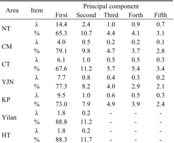
Table 2. Eigenvalues and explained percentages of the principal component for ozone.
Principal component Area Item
First Second Third Forth Fifth λ 14.4 2.4 1.0 0.9 0.7 NT % 65.3 10.7 4.4 4.1 3.1 λ 4.0 0.5 0.2 0.2 0.1 CM % 79.1 9.8 4.7 3.7 2.8 λ 6.1 1.0 0.5 0.5 0.3 CT % 67.6 11.2 5.7 5.4 3.4 λ 7.7 0.8 0.4 0.3 0.2 YJN % 77.3 8.2 4.0 2.9 2.1 λ 9.5 1.0 0.6 0.5 0.3 KP % 73.0 7.9 4.9 3.9 2.4 λ 1.8 0.2 - - - Yilan % 88.8 11.2 - - - λ 1.8 0.2 - - - HT % 88.3 11.7 - - -
λ : eigenvalue; %: the explained percentages.
the summation of effective monitoring stations for varied air-quality districts. Three principles are used for filtering the continuous five-day episode; first, one day with a component score of the first principle component exceeding two; second, the component score of the first principle component during the selected five days should consistently exceed one; third, two preferential episodes were cited.
RESULTS AND DISSCUSSION
According to the result of the principle component analysis, the eigenvalues and attributed
percentages of the first five principle components for
PM10 and ozone were respectively illustrated in
Tables 1 Table 3. The distribution of station-day numbers for PM10.
Station-day numbers Days
Range
NT CM CT YJN KP Yilan HT NT CM CT YJN KP Yilan HT
-1.5 <s< -1 0 0 0 0 1 0 0 0 2 17 44 56 5 4 -1 <s< 0.5 0 0 0 1 0 0 0 98 110 109 72 76 112 88 -0.5 <s< 0 5 1 5 0 6 0 0 147 116 91 83 57 120 140 0 <s< 0.5 4 1 9 10 95 0 0 55 58 56 74 67 61 75 0.5 <s< 1 14 4 63 31 422 0 0 29 37 48 46 65 28 29 1 <s< 1.5 44 9 95 101 356 0 0 15 23 25 28 32 18 9 1.5 <s< 2 76 9 46 72 138 0 0 11 7 7 12 11 9 8 2 <s 185 47 111 64 28 9 1 11 13 13 7 2 13 12 Sum 328 71 329 279 1046 9 1
s presented the component scores of the first principal component.
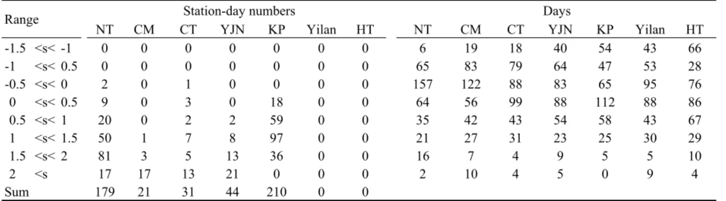
Table 4. The distribution of station-day numbers for ozone.
Station-day numbers Days
Range
NT CM CT YJN KP Yilan HT NT CM CT YJN KP Yilan HT
-1.5 <s< -1 0 0 0 0 0 0 0 6 19 18 40 54 43 66 -1 <s< 0.5 0 0 0 0 0 0 0 65 83 79 64 47 53 28 -0.5 <s< 0 2 0 1 0 0 0 0 157 122 88 83 65 95 76 0 <s< 0.5 9 0 3 0 18 0 0 64 56 99 88 112 88 86 0.5 <s< 1 20 0 2 2 59 0 0 35 42 43 54 58 43 67 1 <s< 1.5 50 1 7 8 97 0 0 21 27 31 23 25 30 29 1.5 <s< 2 81 3 5 13 36 0 0 16 7 4 9 5 5 10 2 <s 17 17 13 21 0 0 0 2 10 4 5 0 9 4 Sum 179 21 31 44 210 0 0
s presented the component scores of the first principal component. Table 5. The correlation coefficients between the
station-day number and the averaged component scores of the first principal component.
Area
NT CM CT YJN KP Yilan HT
O3 0.82 0.68 0.66 0.81 0.84 - -
PM10 0.93 0.85 0.91 0.89 0.94 0.60 -
Table 6. Two cited episodes for ozone and PM10.
Priority Pollutants Date Area
First PM10 1/1~1/5 All Taiwan
Ozone 5/12~5/16 NT 9/18~9/22 Others Second PM10 5/12~5/16 NT, CM 11/23~11/27 CT,YJN,KP 9/18~9/22 Yilan, HT Ozone 6/26~6/30 NT 5/12~5/16 CM 11/23~11/27 CT,YJN,KP 7/25~7/29 Yilan, HT
and 2. The contribution ratios of the first principle
component for PM10 and ozone to different air-quality
areas were at least 79 and 65%. According to principal
component analysis of PM10 , the explained ratios of
the first principle component to NT, CM, CT, YJN, KP, Yilan and HT air-quality areas were respectively, 79, 79, 82, 81, 97 and 80%. The attributed percentages of the second principle component for all of the air-quality areas are less than 9%, except for HT air quality area (this area included just two monitoring stations). From the eigenvalues of ozone in Table 2, the contribution ratios of the first principle component to areas NT, CM, CT, YJN, KP, Yilan and HT were, respectively, 65, 79, 68, 77, 73, 89, and 88%. The second principle component of all the air quality areas explained that the concentration variance was below 12%. Therefore, the first principle component was a suitable indicator for explaining most stations of the concentration variation. Regarding the principle components behind the second principle component,
since their contribution ratios to PM10 and ozone were
lower than 9 and 12%, respectively, and the eigenvalues were smaller than one; they were not suitable indicators for screening air pollution episodes.
The explained contributions of the first component for
PM10 were all larger than for ozone in seven
air-quality basins, which showed the concentration
variance of the first component for PM10 were larger
than ozone over Taiwan.
Reduction in the proportion of unhealthy days was used as the indicator of air-quality management program in Taiwan. To realize the concentration pro-
Table 7. The relation between station-day numbers and the component score of the first principal component for PM10
in the year 2000.
Station-day numbers Component score of the first principal component
Date
NT CM CT YJN KP Yilan HT NT CM CT YJN KP Yilan HT
1/1 1 1 1 2 0.35 1.37 0.50 0.45 -0.03 2.34 0.35 1/2 1 1 0.79 0.71 0.38 0.63 0.40 1.43 1.54 1/3 7 1 7 5 9 1 1.78 1.76 1.75 1.50 0.93 4.01 3.00 1/4 8 3 10 9 13 1.88 2.24 2.41 2.30 1.73 1.92 2.41 1/5 13 4 9 10 6 2.61 2.27 2.30 2.48 0.60 1.86 0.40 11/23 1 8 -0.51 -0.62 -0.20 -0.13 0.89 -0.99 -0.70 11/24 3 1 10 -0.39 -0.16 0.59 0.47 1.16 -0.03 -0.22 11/25 1 6 3 11 -0.33 1.24 2.13 1.36 1.35 0.07 -0.18 11/26 1 8 4 11 0.08 1.33 2.75 1.55 1.64 0.17 -0.24 11/27 3 7 12 -0.21 -0.22 0.97 2.00 1.82 -0.55 -0.27
Table 8. The relation between station-day numbers and the component score of the first principal component for ozone in the year 2000.
Station-day numbers Component score of the first principal component
Date
NT CM CT YJN KP Yilan HT NT CM CT YJN KP Yilan HT
9/18 6 0.75 1.79 1.43 1.61 1.31 2.22 2.08 9/19 1 2 1 2 0.51 2.27 1.76 1.48 1.00 1.20 1.83 9/20 2 5 5 8 0.01 2.55 2.52 2.19 1.53 -0.07 0.64 9/21 1 4 3 4 -0.25 1.72 2.21 2.06 1.20 -0.68 -0.13 9/22 2 3 -0.66 0.09 0.49 1.08 1.37 -1.17 -0.90 11/23 1 1 -0.46 -0.40 0.54 0.31 0.67 -0.82 0.15 11/24 1 3 -0.44 -0.01 0.70 1.39 1.05 -0.40 -0.23 11/25 1 4 5 -0.28 1.43 1.33 2.30 1.30 -0.13 0.45 11/26 2 3 4 0.49 1.10 1.16 1.41 1.27 -0.12 -0.48 11/27 4 -0.45 -0.59 0.41 1.00 1.21 -0.55 -0.34
file of air pollution episodes, this study chose the regulated limits for daily PM10 (125 µg/m3) and hourly ozone (120 ppb) as indicators of severe air pollution. In one day, the daily PM10 value of one station (or the maximum hourly ozone) exceeded the regulatory limit, the station-day number was one; two monitoring stations exceeded the regulatory limit, the station-day numbers were two. After analyzing the distribution of the component score for the first principle component (Tables 3 and 4), the day proportions for the averaged
component score exceeding 1.5 for PM10 were
respectively, 6.0, 5.5, 5.5, 5.2 and 3.6% in areas NT, CM, CT, YJN and KP; however, represented 80, 79, 48, 49 and 16% of the total station-day numbers. As the averaged component score of the first principal component were from 0 to 0.5, there were 55 days cited and the station-day number was 4 in ET area. As for ozone, the day proportions by which the averaged
component score exceeded 1.5 for PM10 were,
respectively, 4.9, 4.6, 2.2, 3.8 and 1.4% in areas NT, CM, CT, YJN, and KP; nevertheless, explained for 55, 95, 58, 77 and 17% of the total station-day numbers.
Comparing different air-quality areas of ozone concentrations, KP and NT were the first and second districts with the highest averaged component scores for the first principal component. In the same component score interval of the first principal component (between 1.5~2.0), the average value of station-day numbers (station-day numbers / days) of ozone in areas NT, CM, CT , YJN and KP were 5.1, 0.4, 1.3, 1.4 and 7.4, respectively; PM10 were 6.9, 1.3, 6.6, 6.0 and 12.6, respectively.
The correlation coefficients (Table 5) between the component score of the first principle component and the station-day numbers exceeded 0.65 for ozone
and 0.85 for PM10 for areas NT, CM, CT , YJN and
KP. Area KP possessed the highest correlation
coefficient for ozone (0.84) and PM10 (0.94), the air
pollution episode of area KP had the highest station-day numbers. Because there were two air-quality stations for areas Yilan and HT, and the station-day numbers were below those for the other five air-quality districts, these two air-air-quality districts could be ignored in the typical results. Correlation analysis
indicated that the correlation between the averaged component scores of the first principle component and station-day numbers were positively and strongly correlated, except for the ozone in areas CM and CT. Consequently, the station-day numbers increased with the averaged component score of the first principle
component and showed that the ozone and PM10
concentrations for most stations were higher than the regulatory limits with the higher component scores of the first component. In conclusion, the component score of the first principle component is a suitable indicator for screening air pollution episodes.
According to the daily component scores and the
exclusion of occurrence day on PM10, this work cited
two alternative episodes for PM10 and ozone. (Table 6)
From Jan. 1 to Jan. 5 in year 2000, PM10 experienced
the most severe episode over Taiwan. The first priority of ozone episode was May 12 to May 16 for area NT, Sep. 18 to Sep. 22 for other six areas. Tables 7 and 8 illustrated the averaged component score of the first principal component, the station-day numbers,
and the selected ozone and PM10 episodes for the year
2000. The highest station-day number of PM10 in area
NT on Jan. 5 was 13 and the highest component score of the first principal component was 2.61. In the same
episode of ozone or PM10, area KP had the highest
station-day numbers than other six areas.
CONCLUSIONS
This study used the component score of the first
component as the indicator for screening the PM10 and
ozone episodes by applying principal component analysis. This indicator can easily select air pollution episodes, and could serve as a reference for future air-quality management or meteorological applications.
The station-day numbers of ozone and PM10 at the
specific date increased with the components score of the first principal components. Meanwhile, this study
provided the concentration distributions of PM10 and
ozone over Taiwan on episode days. The attributed percentages of the first principal components were
greater than 79 and 65% for PM10 and ozone,
respectively. Except for the Yilan and HT air-quality districts, the correlations between the component scores of the first principal components and
station-day numbers for ozone and PM10 exceeded 0.65 and
0.85, respectively. This result demonstrated that the first principal component was the main source of
concentration variance for ozone as well as PM10.
Besides, the station-day number increased with the component score of the first principal component. To sum up, the first principal component was an efficient indicator for selecting air pollution episodes.
REFERENCES
1. TEPA, National Environmental Protection Plan, http://www.epa.gov.tw (2004).
2. U.S. Environmental Protection Agency, “Guideline for Regulatory Application of Urban Airshed Models,“ EPA-450/4-91- 013 (1991).
3. Ames, J., T. C. Mayers, L. E. Reid, D.C. Whitney, S. H. Goldings, S. R. Hayes and S. D. Reynolds, “Airshed Model Operations Manuals, Vol. I, User’s Guide Manual; Vol. II, Systems Manual,” EPA-600/8-85/007a,b.U.S. Environmental Protec-tion Agency, Atmospheric Sciences, Research Laboratory, Research Triangle Park, N.C. (1985). 4. Meyer, E. L., K. W. Baldridge , S. Chu and W. M.
Cox, “Choice of Episodes to Model: Considering Effects of Control Strategies on Ranked Severity of Prospective Episodes Days,” Air & Waste
Management Association’s 90th Annual Meeting & Exhibition 97-MP112.01 (1997).
5. Yang, K. L., “Spatial and Seasonal Variation of
PM10 Mass Concentrations in Taiwan,” Atmos.
Environ., 36, 3403–3411 (2002).
6. Lin, T. H., ”Long-range Transport of Yellow Sand to Taiwan in Spring 2000: Observed Evidence and Simulation.,” Atmos. Environ., 35, 5873-5882 (2001).
7. Kidson, J. W., “Eigenvector Analysis of Monthly Mean Surface Data,” Mon. Wea. Rev., 103, 177-186 (1975).
8. Walsh, J. E. and A. Mostek, “A Quantitative Analysis of Meteorological Anomaly Patterns over the United States, 1900-1977,” Mon. Wea. Rev., 108, 615-630 (1980).
9. Maheras, P., “Weather-type Classification by Factor Analysis in the Thessaloniki Area,” J.
Climatol., 4, 437-443 (1984).
10. Cohn, R. D. and R. L. Dennis, “The Evaluation of Acid Deposition Models Using Principal Component Spaces,” Atmos. Environ., 28, 2531- 2543 (1994).
11. Henry, R. C. and G. M. Hidy, “Multivariate
Analysis of Particulate Sulfate and Other Air Quality Variables by Principal Components-Part I Annual Data from Los Angeles and New York,”
Atmos. Environ., 13, 1581-1596 (1979).
12. Ashbaugh, L. L., L. O. Myrup and R. G. Flocchini, “A Principal Component Analysis of Sulfur Concentrations in the Western United States,”
Atmos. Environ., 18, 783-791 (1984).
and Source Identification for Multispecies Groundwater Contamination,” J. Contaminant
Hydrology, 48, 151–165 (2001).
14. Statheropopulos, M., N. Vassiliadis and A. Papps, “Principal Component and Canonical Correlation Analysis for Examining Air Pollution and Meteorological Data,” Atmos. Environ., 32, 1087-1095 (1998).
15. Henry, R. C. and G. M. Hidy., “Multivariate Analysis of Particulate Sulfate and Other Air Quality Variables by Principal Components-part II Salt Lake City,” Utah and ST. Louis, Missouri,
Atmos. Environ., 16, 929-943 (1982).
16. Poissant, L., J. W. Bottenheim, P. Russell, N. W. Reid and H. Niki, “Multivariate Analysis of a 1992 Sontos Data Subset,” Atmos. Environ., 30, 2133-2144 (1996).
17. Verbeke, J. S., J. C. D. Hartog, W. H. Dekker, D. Coomans, L. Buydens and D. L. Massart, “The Use of Principal Component Analysis for the Investigation of an Organic Air Pollutants Data Sets,” Atmos. Environ., 18, 2471-2478 (1984).
18. Yu, T. Y. and L. F. W. Chang, “Selection of the Scenarios of Ozone Pollution at Southern Taiwan Area Utilizing Principal Component Analysis,”
Atmos. Environ., 34, 4499-4509 (2000).
19. Yu, T. Y., L. F. W. Chang, “Delineation of Air Quality Basins Utilizing Multivariate Statistical Methods in Taiwan,” Atmos. Environ., 35, 3155-3166 (2001).
20. Taiwan Environmental Protection Administration, “The Management Plan of China Dust Storms,” EPA-92-FA11-03- B007 (2003).
Discussions of this paper may appear in the discussion section of a future issue. All discussions should be submitted to the Editor-in-chief within six months.
Manuscript Received: September 1, 2004 Revision Received: December 26, 2004 and Accepted: December 29, 2004