黏著劑結合之接頭應力分析及其在取晶過程之應用

國 立 交 通 大 學

機 械 工 程 研 究 所

博 士 論 文

黏著劑結合之接頭應力分析及其在取晶過程之應用

Stress Analysis of the Adhesively Bonded Joint

Applicable to the IC Chip Pick-up Process

研 究 生： 鄭 桐 華

指導教授：洪 景 華 教授、曾 錦 煥 教授

中華民國九十五年十二月

黏著劑結合之接頭應力分析及其在取晶過程之應用

Stress Analysis of the Adhesively Bonded Joint Applicable

to the IC Chip Pick-up Process

研 究 生：鄭 桐 華

Student: Tung-Hua Cheng

指導教授：洪 景 華 Advisor:

Ching-Hua

Hung

曾 錦 煥

Ching-Huan Tseng

國立交通大學

機械工程研究所

博士論文

A Dissertation

Submitted to Institute of Mechanical Engineering

College of Engineering

National Chiao Tung University

in Partial Fulfillment of the Requirements

for the Degree of

Doctor of Philosophy

in

Mechanical Engineering

2006

Hsinchu, Taiwan, Republic of China

中 華 民 國 九十五 年 十二 月

黏著劑結合之接頭應力分析及其在取晶過程之應用

研究生：鄭桐華

指導教授：洪景華教授、曾錦煥教授

國立交通大學機械工程研究所

ABSTRACT (中文摘要)

摘

要

本文主要探討一黏著劑(adhesive)接合二個黏著物(adherends)在銷-銷(pin-pin)之邊界 條件(boundary conditions)下受到集中力(concentrated force)作用，在此條件下導出其統 御 方 程 式 (governing equations) 為 複 雜 之 偶 合 方 程 式 (coupled equations) ， 其 解 析 解 (analytic solutions)利用符號運算(symbolic manipulation)求得，並使用奇異值分解法 (singular value decomposition, SVD)求得符合邊界條件之數值解。

文中討論黏著層(adhesive layer)的剝離應力(peel stress)及剪應力(shear stress)受到黏 著物及黏著劑之材料性質、幾何形狀(厚度、長度)、接合長度、力作用點等的影響。在 無因次化參數(non-dimensional parameter) 的值為E₁=6.0, E2=6.0, E0=2.75, P

~

=1, 及參數 d = 0 的情形下，對於上層黏著物(upper adherend)能夠從下層黏著物(lower adherend)完全 分離，必須滿足下面的條件，下層黏著物的厚度大於 10 倍的黏著層之厚度且小於 1/3

上層黏著物之厚度，並且黏著層厚度相對的薄(h_a ≤0.01 mm)，接合時，其長度相對的

短，也就是說厚長比(thickness to length ratio)大於 0.08 (γ₁≥0.08)。

接著將上述黏著接頭之分析(analysis of adhesive joint)方法結合 C++語言的基因演算 法(genetic algorithm)運用於取晶過程之探討。當 0.1mm 厚的晶片受到 4.8N 的集中力， 取晶良率(success rate)很低，且晶片不是破裂就是無法從藍膜(blue tape)分離。但當 0.34mm 厚的晶片受到 3.5N 的集中力，取晶良率很高，且晶片幾乎没有破裂且可以完 全成功的從藍膜分離。對這二實驗中，其取晶良率差異很大。本文利用基因演算法結 合黏著接頭之分析方法去找尋黏著劑之材料性質。對 0.1mm 厚晶片的例子中，當黏著 劑的厚度為 0.01mm 時，完全尋找不到材料性質符合之黏著劑。另外本文希望以不同的 黏著劑的厚度來改善晶片厚度為 0.01mm 的取晶良率，但是結果也完全找尋不到材料性 質及厚度符合之黏著劑，但是對晶片厚度為 0.34mm 的例子，當黏著劑的厚度為

0.01mm 時，就可以找尋到黏著劑的彈性係數(Young’s modulus)為 pa，而且本

文希望以一般黏著劑取代實驗所使用的輻射黏著劑(radiation-cured adhesives)或稱為紫 外 線 黏 著 劑 (ultra-violet adhesive) 時 ， 也 可 找 到 黏 著 劑 的 彈 性 係 數 及 厚 度 分 別 為 pa 及 0.027mm。這些理論分析的結果一致於實驗的結果。 10 10 46 . 2 × 10 10 77 . 2 × 為了改善先前例子，對晶片的厚度為 0.1mm 易於破裂或無法從藍膜分離，藍膜的彈 性係數必須再予增加。只要藍膜的彈性係數大於 1/10 倍的晶片之彈性係數，皆可找得 到黏著劑的彈性係數及厚度值，且其畸變能應力(von Mises’s stresses)皆大於 130Mpa， 超過一般黏著劑的臨界應力(40-80Mpa) [51]，因此可預知當厚度 0.1mm 的晶片在取晶 時，改變藍膜的材料性質，就能夠提高從藍膜成功分離之機會。

Stress Analysis of Adhesively Bonded Joints Applicable to

the IC chip pick-up Process

Student: Tung-Hua Cheng

Advisor: Ching-Hua Hung

Ching-Huan

Tseng

Institute of Mechanical Engineering

National Chiao Tung University

ABSTRACT

In this study, a concentrated force is applied to both adherends bonded by an adhesive under the pin-pin boundary conditions. First a mathematical model is derived with governing equations and boundary conditions. These complicated, and analytically problematic, coupled equations are solved numerically using symbolic manipulation and singular value decomposition (SVD). Also discussed are the effects of major factors, including the relative thickness of, material properties of adherends and adhesive, joint length, and the action point of the concentrated force on the peel and shear stresses in the adhesive layer. As non-dimensional parametersE1=6.0, E2 =6.0, E0 =2.75, P

~

=1 and the parameter d = 0, this study identifies the conditions under which the upper adherend without breakage can be fully separated from the lower adherend. Particularly, it is found that the thickness of the lower adherend should be greater than ten times that of the adhesive layer but less than one-third that of the upper adherend, the adhesive layer should be relatively thin ( mm), and the adhesive joint should be relatively short (thickness to length ratio

01 . 0 ≤ a h 08 . 0 1 ≥ γ ).

Subsequently, the aforementioned analysis of adhesive joint is associated with the C++ program of genetic algorithm and is applied to investigate IC chip pick-up process. As the thickness of IC chips subjected to the concentrated force 4.8 N is 0.1 mm, IC chips are easy to fail in the IC chip pick-up process while as the thickness of IC chips subjected to the concentrated force 3.5 N is 0.34 mm, IC chips are fully separated from blue tape without breakage. The two experiments have a great difference in the success rate of the IC pick-up process. The experimental results are discussed by genetic algorithm searching associated

with analysis of adhesive joint. The former case is as the thickness of the adhesive layer is 0.01mm, the solution to Young’s modulus of the adhesive layer is not found. Additionally, it is expected that the success rate of the IC pick-up process can be raised by changing the adhesive’s thickness. However, the searching result does not also find any solution to material properties and thickness of adhesive. The latter case is as the thickness of the adhesive layer is 0.01mm, Young’s modulus of the adhesive layer is searched and the value of Young’s modulus obtained is pa. In addition, it is expected that in the IC pick-up process, radiation-cured adhesives (ultra-violet adhesives) can be replaced by general adhesives. The searching result can also obtain Young’s modulus of and the thickness of the adhesive layer which are respectively pa and 0.027mm. These results are in accordance with those of the experiments.

10 10 46 . 2 × 10 10 77 . 2 ×

In order to reduce the easy failure of the former case regarding IC chip’s thickness 0.1 mm, the Young’s modulus of blue tape has to be increased. The conclusions are that only if the Young’s modulus of blue tape is greater than one-tenth that of IC chips, genetic algorithm can obtain the searching results of adhesive’s Young’s modulus and adhesive’s thickness. Thereby, only if the mechanical properties of blue tape are changed, the probability of IC chips which can be fully separated from blue tape is expected to be able to increase because the von Mises’s stresses of the searching results are greater than 130Mpa exceeding the critical value (40-80Mpa) [51] of general adhesive.

ACKNOWLEDEMENTS

本人在此以最誠摯的敬意向曾錦煥博士及洪景華博士表示最大的謝意，感謝他們 在我攻讀博士學位期間無私的付出與真摯的關懷，這份恩情本人永生難忘。在這期間 指導教授曾錦煥博士不幸離世，更感謝洪景華老師能夠繼續給我支持、鼓勵，讓我能 夠順利完成博士學位。 其次，感謝論文口試委員：清華大學賀教授陳弘、前國科會工程處處長─明新科 技大學蔡教授忠杓、交通大學機械系周教授長彬、台灣大學呂教授東武、國防大學林 教授聰穎，謝謝他們在百忙之中，不辭辛勞，撥冗前來擔任我的論文口試委員，並給 我在論文寫作上許多寶貴的建議，同時提供相關的研究經驗，讓我的論文能夠更加完 整與充實。 再者，感謝師母姚女士的幫忙及關懷，更感謝諸多朋友的幫忙，並對這些朋友致 上最高的謝意。本人特別要感謝各位學長學弟的鼎力協助，讓我對這段新竹攻讀學位 的日子留下不可忘懷的記憶，另外也一併感謝最佳化實驗室的師門兄弟諸多的幫助。 此外，感謝英文老師涂清欽老師及李佩倫老師，百忙之中特別撥出時間，耐心地 幫忙潤飾我的論文。 我敬愛的母親─鄭林幼字女士於我大二時往生西方極樂，我敬愛的父親─鄭義立 先生，在我攻讀博士期間離世，讓我悲痛萬分。想起父母親為我所做的點點滴滴，銘 記在心，永生難忘。 我心中最感謝的是一路相伴我的妻子─翁淑玲女士。幾年來，她不畏艱辛，支持 我、陪伴我，渡過漫長的求學生涯，協助我順利完成博士學位，同時細心地照顧我年 邁的父親、兩個稚子─光庭、光祐。感謝岳父母的鼓勵及姊姊的幫助，我要以這份論 文獻給我摯愛的妻子、孩子、岳父母及姊姊。 最後，在攻讀學位期間，我的父親鄭義立、老師曾錦煥往生西方極樂，我要以此 論文紀念我的父親鄭義立先生、母親林幼字女士及老師曾錦煥博士，感謝他們對我的 教導。

TABLE OF CONTENTS

ABSTRACT (中文摘要) ...i

ABSTRACT ...ii

ACKNOWLEDEMENTS ...iv

TABLE OF CONTENTS ...v

LIST OF TABLES ... viii

LIST OF FIGURES ...ix

NOMENCLATURE ...xii CHAPTER 1 INTRODUCTION...1 1-1. Background ...1 1-1-1. Adhesive ...2 1-1-2. Joint Type...3 1-2. Objectives...10

1-3. Significance and Limitations...11

1-4. Dissertation Outlines ...12

CHAPTER 2 LITERATURE REVIEW...14

2-1. Introduction ...14

2-2. Adhesively Bonded Joints...14

2-2-1. Introduction...14

2-2-2. Thermal Loading...15

2-2-3. Anisotropic and Orthotropic Materials ...16

2-2-5. Plastic Behavior of Adhesive Joints ...17

2-2-6. Crack Analysis and Stress Singularity...17

2-2-7. Strengthening Structures...18

2-3. Genetic Algorithm and Penalty Function Method ...18

2-3-1. Introduction...18

2-3-2. Penalty Function Method without Any Penalty Parameters ...19

2-3-3. Adaptive Search Techniques...20

2-3-4. Genetic Algorithm Application to Adhesively Bonded Joints ...21

2-4. Methods Applied to Solve the Issues of Adhesively Bonded Joints...21

2-5. Concluding Remarks ...23

CHAPTER 3 ANALYSIS OF ADHESIVE JOINT ...25

3-1. Introduction ...25

3-2. Mathematical Model ...25

3-2-1. Bending moment, Shear force, and Longitudinal Force in the Upper Adherend and Lower adherend...27

3-2-2. Relationship between Displacement and Stress...31

3-2-3. Relationships among Displacement, Longitudinal Force, and Bending Moment...32

3-3. Non-dimensionalization and Symbolic manipulation ...34

3-4. Constraint and Boundary Conditions ...40

3-5. Results and Discussion...42

3-5-1. Application of Closed-form Solutions ...42

3-5-2. Case Studies ...45

3-7. Concluding Remarks ...62

CHAPTER 4 APPLICATION OF GENETIC ALGORITHM TO IC CHIP PICK-UP PROCESS...63

4-1. Introduction ...63

4-2. Optimum problem ...65

4-3. Results and Discussion...69

4-4. Concluding Remarks ...72

CHAPTER 5 CONCLUSIONS AND FUTURE WORKS ...75

5-1. Conclusions ...75 5-2. Future works...78 REFERENCES ...80 APPENDICES ...86 Appendix A ...86 Appendix B...94 Appendix C...97 Appendix D ...104 VITA...108

LIST OF TABLES

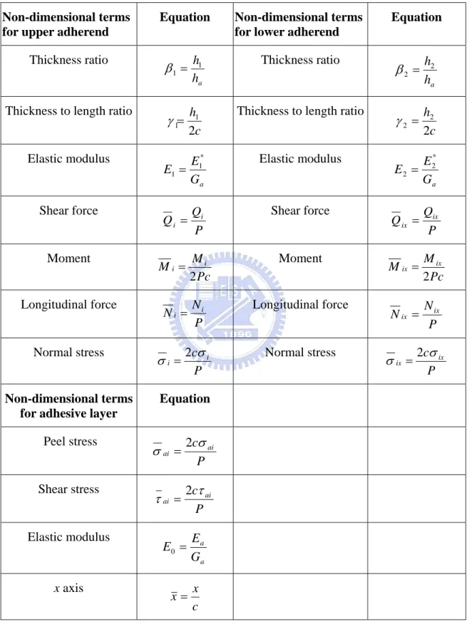
Table 3.1 The non-dimensional terms and equations for upper adherend, adhesive layer and lower adherend. ...39 Table 4.1 Mechanical properties and dimensions for IC chip and blue tape. [45],[52] ....67 Table 4.2 Optimum points and values of adhesive for various Young’s modulus of blue tape

LIST OF FIGURES

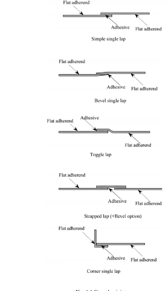
Fig. 1.1 Singe lap joints ...5

Fig. 1.2 Butt joints ...6

Fig. 1.3 Double lap joints ...6

Fig. 1.4 Scarf lap joints...7

Fig. 1.5 Stress catalogy...7

Fig. 1.6 Processes in the IC manufacturing procedure. [1] ...9

Fig. 1.7 Two adherends of the adhesively bonded joint bonded by an adhesive layer. ....10

Fig. 3.1 The sketch showing two adherends bonded by an adhesive layer. ...25

Fig. 3.2 Free-body diagram for the first segment −L₁ ≤ x≤−c, of lower adherend...27

Fig. 3.3 Free body diagram for the second segment −c≤x≤−d, of lower adherend. ...28

Fig. 3.4 Free body diagram for the third segment −d ≤ x≤c, of lower adherend ...28

Fig. 3.5 Free body diagram for the fourth segment of c≤x≤L₂, of lower adherend...28

Fig. 3.6 Free body diagram for the first segment −c≤x≤−d, of upper adherend. ...30

Fig. 3.7 Free body diagram for the second segment −d≤x≤c, of upper adherend. ...31

Fig. 3.8 The sketch of the Cornell’s model [29] showing cantilever beam strengthened by adhesively bonding ...43

Fig. 3.9 Comparison of the results between the present study (top) and figure 6 of the Cornell’s paper [29] (bottom)...44

Fig. 3.10 The sketch of the Zou et al. model [30] showing a single lap joint ...45

Fig. 3.11 Comparison of the results between figure 5 of the Zou et al.’s paper [30] and the present study. ...45

Fig. 3.12 Non-dimensional peel and shear stresses distributions in the adhesive layer (x = x/c) for the thickness to length ratio γ =γ₁ =γ₂ with the same thickness of both adherends β₁ =β₂ =10and (h_a =0.01mm) ...48

Fig. 3.13 Non-dimensional peel and shear stresses versus the thickness to length ratio

2 1 γ

γ

γ = = for the same thickness of the adherends as for Case 1 (h_a =0.01mm). 49

Fig. 3.14 Non-dimensional peel and shear stress distributions in the adhesive layer (x =x/c) versus the thickness to length ratioγ₁ for various thicknesses of the adherends for Case 2, (h_a =0.01mm). ...52 Fig. 3.15 Non-dimensional peel and shear stresses versus the thickness to length ratio of the

upper adherend γ₁ for various thicknesses of the adherends for Cases 2 and 3. ...53 Fig. 3.16 Non-dimensional peel and shear stress distributions for the distance d from the

center of the adhesive layer to the action point of the force (h_a =0.01mm, γ =0.01667). ...55 Fig. 3.17 Non-dimensional peel and shear stress distributions for different distances d from

the center of the adhesive layer to the action point of force (ha =0.02mm, γ =0.05). ...56 Fig. 3.18 Non-dimensional peel and shear stresses distributions in the adhesive layer

(x = x/c) for Young’s modulus ratio with the same thickness of both adherends 10

2 1 =β =

β and (ha =0.01mm) ...57

Fig. 3.19 Non-dimensional peel and shear stresses versus the adhesive Young’s modulus ratio with the same thickness of both adherends β₁ =β₂ =10and (h_a =0.01mm)...58 Fig. 3.20 Non-dimensional peel and shear stresses distributions in the adhesive layer

(x = x/c) for the thickness to length ratio γ =γ₁ =γ₂ with the different Young’s modulus of both adherends E₁ =4.5, E₂ =6.0, E₀ =2.75and with the same thickness of both adherends β₁ =β₂ =10and (h_a =0.01mm)...59

Fig. 3.21 Non-dimensional peel and shear stresses versus the thickness to length ratio

2 1 γ

γ

γ = = for the same thickness of the adherends with the different Young’s modulusE₁ =4.5, E₂ =6.0, E0 =2.75 (ha =0.01mm). ...60 Fig. 4.1 Scheme of genetic algorithm linked with Mathematics package to compute stresses of

NOMENCLATURE

c

Half length of the joint bonded by the adhesive(i.e. 2c length of upper adherend) C Denotation of cos(α₁₂x)

Ch Denotation of cosh( xα )

1

Ch Denotation of cosh(α₁₁x)

d

Distance from the action point of force to the center of the joint

* 1

E Elastic modulus of the upper adherend

a

E Elastic modulus of the adhesive layer

1

E The ratio of elastic modulus of the upper adherend to shear modulus of the adhesive

layer

0

E The ratio of elastic modulus of the adhesive layer to shear modulus of the adhesive

layer

2

E The ratio of elastic modulus of the lower adherend to shear modulus of the adhesive

layer

* 2

E Elastic modulus of the lower adherend

1

E Elastic modulus of the upper adherend in plane stress

2

E Elastic modulus of the lower adherend in plane stress

F

L Reaction force in the left-end pin boundary of the lower adherend

F

R Reaction force in the right-end pin boundary of the lower adherend

a

G Shear modulus of the adhesive layer

h

1 Thickness of the upper adherend

h

a Thickness of the adhsive layer

h

b Thickness of the adhsive layer in Cornell’s paper[29]

h

2 Thickness of the lower adherend

L

1 Distance from the center of joint to the left end of the lower adherend

L

2 Distance from the center of joint to the right end of the lower adherend

M

ix Bending moment in the i segment of the lower adherend

N

ix Longitudinal force in the i segment of the lower adherend

M

i Bending moment of the upper adherend

i

M Non-dimensional moment of the upper adherend

ix

M Non-dimensional moment of lower adherend

N

i Longitudinal force of the upper adherend

N

L Longitudinal force in the left-end pin boundary of the lower adherend

N

R Longitudinal force in the right-end pin boundary of the lower adherend

i

N Non-dimensional longitudinal force of the upper adherend

ix

N Non-dimensional longitudinal force of the lower adherend

Q

i Shear force of the upper adherend

Q

ix Shear force in the i segment of the lower adherend

Q

i Shear force of the upper adherend

i

Q Non-dimensional shear force of the upper adherend

ix

Q Non-dimensional shear force of the lower adherend

R

Penalty parameter.

S

Denotation of sin(α₁₂x)

Sh

Denotation of sinh( xα ) 1

Sh

Denotation of sinh(α₁₁x) ix

i

u

Longitudinal deformation in the i segment of the upper adherend ix

w

Transverse deformation in the i segment of the lower adherend

i

w

Transverse deformation in the i segment of the upper adherend

x

x-axis coordinate

z

z-axis coordinate

σ

Non-dimensional peel stress of the adhesive layer

0

σ

Non-dimensional peel stress of the adhesive layer in the center

1

σ

Non-dimensional peel stress of the adhesive layer at both ends

ai

σ

Peel stress in the i segment of the adhesive layer

ai

τ

Shear stress in the i segment of the adhesive layer

ai

σ

Non-dimensional peel stress in the i segment of the adhesive layer

ai

τ

Non-dimensional shear stress in the i segment of the adhesive layer

τ

Non-dimensional shear stress of the adhesive layer

1

τ

Non-dimensional shear stress of the adhesive layer at both ends

12 11

,

,

α

α

α

The solutions of the characteristic Eqns.

1

β

The ratio of the thickness of the upper adherend to the thickness of the adhesive layer

2

β

The ratio of the thickness of the lower adherend to the thickness of the adhesive layer

1

γ

The ratio of the thickness of the upper adherend to the length of the adhesive layer

2

γ

The ratio of the thickness of the lower adherend to the length of the adhesive layer

1

2

ν

Possion’s ratio of the lower adherend

x

Non-dimensional coordinate (x/c)

λ

The ratio of Young’s modulus of the upper adherend to Young’s modulus of the adhesive layer

CHAPTER 1 INTRODUCTION

1-1. Background

As technology advances, use of adhesives is becoming ever more widespread because adhesive can also help make it easier to manufacture products and be used extensively to bond metallic, ceramic, plastic and composite components in many fields where structures are subject to high levels of service. Therefore, nowadays, product designers and manufacturing engineers rely on adhesives more than ever for greater design flexibility, more efficient production, and improved performance. In addition, adhesives applied to joints have been used for many years in aircraft structures and in many other applications including particular aircraft repair, civil engineering, automotive engineering, medical field, and the electronics industry.

Adhesive bonding has many advantages over the conventional fastening techniques such as welding, riveting and bolting because its application does not require high temperatures in welding and hole in structure component like the cases of riveting and bolting. Thereby, stress concentration in the adhesive joints is less than that caused by high temperature of welding as well as hole of rivets and bolts; stress distributions of adhesive joints are more uniform. Additionally, using adhesive bonding has the substantial benefit of weight reduction that is an important advantage, especially for lightweight structures. Therefore, the use of adhesive materials as a means for assembly of structure is being accepted as an alternative means to conventional joining processes. Except weight reduction, the advantages of structural adhesive bonding over other joining techniques include cost savings (including lower labor costs), elimination of stress point concentrations by even more uniform distribution of stress over the entire bonded joint described above, bonding of dissimilar materials, and resistance to shock as well as vibration et al.. In Addition, adhesive bonding applied to composites is

being increasingly used in structural applications, which is also justified by its well-known advantages over mechanically fastened joints: fewer sources of stress concentrations, more uniform distribution of load, and better fatigue properties. Hence, the use of adhesives is more widespread than ever in technically demanding applications.

Though adhesive bonding has many aforementioned advances and great potential, it, however, results in some inconveniences. For instance, adhesive bonding is almost always irreversible; in other words, to disassemble the bonding without damaging the structural components is not easy.

1-1-1. Adhesive

As for adhesively bonded joints applied to structure component, adhesive selection is very important. The selection criteria are based upon material information, joint type and loading condition et al.. Material information involves the characteristics of adhesives and adherends as well as the boned strength of adhesive. Understanding these characteristics is very important for selecting suitable adhesive employed in bonded joints. Because there is a great variety of adhesives over 18 different generic types of adhesives as well as numerous sub-types and hybrids of the adhesive, the selection of the most suitable adhesive for the adhesive joint probably is one of the most daunting areas in the design process.

In this research, only radiation-cured adhesives are introduced because they are often applied to the IC chip pick-up process. They become active and cured when exposed to radiation, usually ultra-violet (UV) light. The mechanism depends upon special modifications to the monomer's structure and the inclusion of light-sensitive compounds that start the reaction. Also, they are also widely used for bonding glass, ceramics and transparent plastics. However, some tapes of radiation-cured adhesives are applied to the IC pick-up process.

These adhesives make it possible to achieve a higher tack before the exposure of UV light while ensuring the easy removal of the adhesives and the reduction of boned strength after exposure. That is to say, as exposure to UV light source breaks adhesive bond, the tack of the adhesive can be reduced. Specially, the adhesives offer worse resistance to peel force.

1-1-2. Joint Type

There are many sub-types of single lap joints as shown in. Generally speaking, single lap joints are the simplest joint geometry and usually used in structural joints but its shortcoming is that peel stresses still arise in this joint. Other joint geometries may be considered to reduce peel stresses; for example, butt joint, double lap joint and scarf joint as shown in Figs 1.2, 1.3 and 1.4 are better selection to reduce peel stresses. Especially, as scarf joints allow a large adhesive contact area, the joint is an ideal joint for eliminating peel stresses, but parts joined in this way must maintain a close fit; however, in practice these joints are harder to create and are not suitable for use with thin sheet adherends.

Joint design requires selection of the correct joint types depending on loading condition, geometrical shape and assembly procedures. Joint design should minimize stress concentrations by ensuring that the load is distributed over the entire bonded area. Some stresses, such as peel, cleavage, and shear stresses, should be minimized (see Fig. 1.5) because these stresses will cause the failure of adhesive joint. Most adhesives applied to structure components withstand tensile stress well, so maximizing the tensile stress and minimizing others is one of the vital targets in designing the structure components but the tensile stress is less than the critical stress of adhesives. Joint type should serve to improve bond strength. It may be important to choose the most suitable joint type of geometrical structures because this joint type minimizes the peeling or shear stresses at the edges of the

overlap in the well-bonded situation. Nevertheless, in the IC chip pick-up process, it is expected that at the edges of joint, the peeling and shear stresses can be maximized and their values also can exceed the critical stresses of adhesive; and IC chips whose stress distribution can be minimized do not fail during the process.

Fig. 1.2 Butt joints

Fig. 1.3 Double lap joints

Fig. 1.4 Scarf lap joints

Fig. 1.5 Stress catalogy

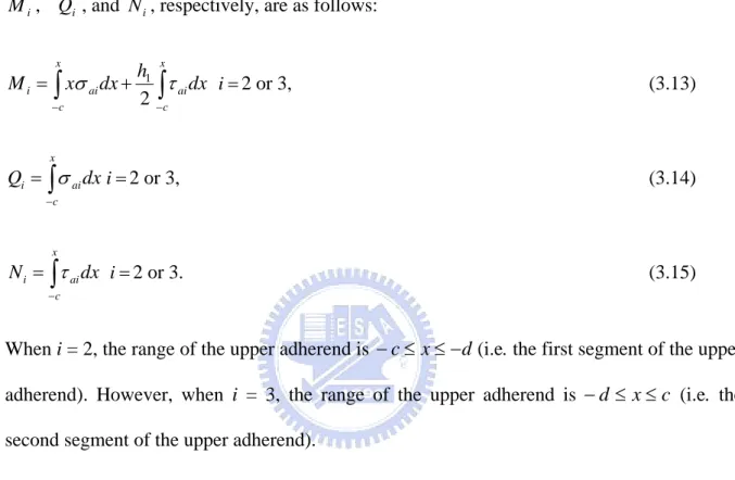
Fig. 1.6 depicts the IC manufacture procedure [1], to elucidate the causes of failure. A wafer is stuck in tape, and polished thinner and flatter. Then, it is removed from the tape and

stuck to the blue tape. The wafer can be fixed to the blue tape by radiation-cured adhesive, and cut into pieces (called IC chips) by a diamond cutter. Sequentially, in the IC chip pick-up process, the IC chips must be pierced and broken off by using the piercer, before being separated from the blue tape without any cracks. However, as IC chips are getting shorter and thinner, IC chips easily fail during IC manufacture. As shown in Fig. 1.7, adhesively bonded joint is applied to IC chip pick-up process. In the adhesively bonded joint, both adherends subjected to a concentrated force, are bonded by an adhesive under the pin-pin boundary conditions. Because its joint type is different from the aforementioned joint types but this joint is a three-laminar structure which is similar as that of a single lap joint, this dissertation mainly investigates the joint. Specially, joint’s adherends are consisted of different materials.

To sum up, the use of adhesively bonded joint keeps increasing but there are still some important issues, such as stress distributions of the joints, to be explored. In this study, the stress distributions of the joints are affected by the key factors which involve the consideration of a variety of geometries, material properties of adhesive and blue tape, and loading conditions.

To perform stress analysis requires reliable and efficient closed-form solutions (analytical solutions) to obtain stress distribution of bonded joints. A large variety of models have been developed to analyze the adhesively bonded joint. Some of these techniques yield closed-form solutions, which generally involve some simplified assumptions. Many of them are limited to a certain range of geometries or loading conditions. Therefore, symbolic manipulation was employed to derive the reliable, efficient and complicated closed-form solutions which can be linked by the C++ program of genetic algorithm. Though finite element methods have provide a general tool to analyze arbitrary geometries and loading conditions, and have been extensively used with success, however, this kind of method requires much finer meshing in the issue and a large set of nodes in order to obtain reasonably accurate results. This needs a

large investment in engineering time and computer resources.

Adhesive layer Upper adherend

Lower adherend

Fig. 1.7 Two adherends of the adhesively bonded joint bonded by an adhesive layer.

1-2. Objectives

The main objective of this study is to derive closed-form solutions (analytic solutions) linked with the C++ program of genetic algorithm to predict the behavior of the adhesively bonded joint in the IC chip pick-up process. To achieve the main objective, the following objectives are indispensable:

1. To obtain closed-form solutions (analytic solutions) to peeling and shear stresses for the adhesive layer, and to normal stress due to bending moment and longitudinal force of adherends as well as to displacement and slope of adherends.

2. Close-form solutions applied to cantilever beam strengthened by adhesively bonding and a single lap joint.

3. The effect of geometric shapes, action point of concentrated force and material properties of adhesive and adherends on peeling and shear stresses.

4. Examining whether adhesive joints are in the well-bonded situation or not.

5. To apply Genetic algorithm linked with analysis of adhesive joint in the IC chip pick-up process, and to discuss the analytical results and experimental results.

1-3. Significance and Limitations

In this study, a concentrated force is applied to both adherends bonded by an adhesive under the pin-pin boundary conditions. The aim of the proposed research is to attain closed-form solutions that will include the most relevant factors of the adhesively bonded joint. These solutions are able to be linked with the C++ program of genetic algorithm since it is still somewhat difficult to converge and directly solve the differential equations by using the numerical method. However, Cornell [29], who claimed that obtaining complete theoretical solutions (closed-form solutions) to this problem would be very difficult, only considered a cantilever beam consisting of the same adherends. Only if the characteristic solutions of these equations have considerable values can his method produce classical solutions for the differential equations. As obtaining analytical solutions (closed-form solutions) is even more difficult here than in the work of Cornell [29], the model uses symbolic manipulation to solve the coupled differential equations in the Mathematica package, thereby enabling to find complete and complicated solutions that are not limited to solving only the characteristic solutions having large values (i.e. the characteristic solutions had to have large values [29]).

Estimating the peel and shear stresses of the adhesive between the IC chip and the blue tape is very important for the adhesive joint in the IC chip pick-up process. The results found in the experiments [45] are that as the thickness 0.1 mm of IC chips subjected to 4.8N, IC chips are easy to fail while as thickness, 0.34 mm of IC chips subjected to 3.5N, IC chips without crack can completely be separated from the blue tape. These closed-form solutions may be applied to analyze the behavior of adhesive in IC chip pick-up process. Therefore, genetic algorithm associated with these closed-form solutions aims to seek the suitable characteristic of adhesive material and blue tape to be able to reduce the failure of IC chips in the IC chip pick-up process. This research shows that conclusions drawn can increase the

success rate of IC chips which without crack, can be successfully separated from blue tape during IC chip pick-up process.

The closed-form solutions are only applied to a single lap joint. Adhesively bonded joint must be based on linear and elastic theory as well as small-deflection (Euler) beam theory under small deflection assumption.

1-4. Dissertation Outlines

In order to carry out the objective described before, the following chapters further illustrate how to accomplish the targets in more details. Here these chapters are briefly introduced in this section. Chapter 2 is devoted to discussing the related literatures regarding adhesively bonded joints and genetic algorithm. In regard to adhesively bonded joints, some published papers, basing on thermal or external load, material properties, plastic behavior, crack analysis, and strengthening structure, are introduced in order. As for genetic algorithm, here discuss some articles including penalty function, adaptive search techniques and its application to adhesively bonded joint. Next, some methods employed to solve the adhesively bonded joint are investigated.

Chapter 3 is dedicated to analysis of adhesive joint and mainly develops theoretical model of the adhesively bonded joint applied to the IC chip pick-up process. The use of symbolic manipulation is employed to solve the closed-form solutions (analytical solutions) to the adhesively bonded joint. These closed-form solutions involve the expressions of the transverse and longitudinal displacements, longitudinal and shear forces, moment in the adherends as well as peel and shear stress of the adhesive. These expressions are also shown to be correct by re-substituting them into coupled differential equations and by comparing the

results of the examples in references [29-30] with those obtained by the application of the expressions to solving those examples.

Sequentially, the IC chip pick-up problem is solved by using these closed-form solutions on which boundary and constraint conditions are imposed. Then, under some conditions, examine whether adhesively bonded joints are in the well-bonded situation or not.

Chapter 4 focuses on comparing the results of the experiments [45] with those of the analysis of adhesive joint and drawing conclusions which can increase the success rate of IC chips in the process. In the experiments, because of the different thicknesses, 0.1mm, and 0.34mm of IC chips, the success rate of the IC chip pick-up process has a great difference. The 0.1mm IC chips nearly fail in slower speed but the 0.34mm IC chips without breakage can almost be completely separated from blue tape. These phenomena are discussed by theoretical model. However, because the characteristics of the adhesive layer are not easily found, genetic algorithm with penalty function, associates with analysis of adhesive joint method to solve the thickness and mechanical properties of the adhesive layer. The program of the genetic algorithm is written by the C++ language. Some conditions are proposed to improve the success rate in the pick-up IC process.

Chapter 5 draws conclusions and discussions about further works of this study in the future.

CHAPTER 2 LITERATURE REVIEW

2-1. Introduction

Based on some aforementioned facts, the design structure involves adhesively adhesive joints, and IC chip as well as blue tape stuck together by adhesive. Strictly speaking, in IC chip pick-up process, an adhesively bonded joint includes two adherends – the IC chip (upper adherend) and the blue tape (lower adherend) bonded by an adhesive in the IC chip pick-up process. In the published articles, many methods have been applied to solve the problems of adhesively bonded joints. Generally speaking, there are mainly several basic approaches, such as finite element method (FEM), numerical method and analytical method, which are often employed to solve the problems of adhesively bonded joints. These approaches are also applied to the following literature and will be discussed in the next sections.

2-2. Adhesively Bonded Joints

2-2-1. Introduction

Adhesively bonded single-lap joints have been widely studied since the 1950s. One of the most widely quoted papers on stresses in adhesive joints is that of Goland and Reissner [2]. Goland and Reissner have developed the cemented-lap mathematical model and found the explicit solutions (closed-form solutions) to two limiting cases. One case is that the cement layer must be so thin that its effect on the flexibility of the joint may be neglected; the other case is that the joint flexibility results mainly from that of the cement layer.

Some studies that have used and extended the Goland-Reissner theory and have compared their own results with Goland-Reissner’s are described below. Oplinger [3] has released the limit of large adherend-to-adhesive layer thickness ratio to obtain the results of the

Goland-Reissner analysis. Oplinger’s model should give the most accurate results for any overlap joint length because the edge moment expression was obtained by considering the large deflections of all the components of the single lap joint structure. Carpenter [4] has verified the correctness of Goland-Reissner’s formulations by making comparisons between his finite element results and the results of Goland-Reissner’s original equations. Ojalvo and Eidinoff [5] have used a more complete shear-strain/displacement equation to solve the single-lap adhesive joints. They explained that the shear stress is the highest value at two anti-symmetrical adherend-bound interface points of the layer; the growth of joint failures originating from these points are consistent with the results obtained from actual experiments. Carpenter [6] summarized the theories of lap joint behavior of Goland and Reissner and of Ojalvo and Eidinoff’s equilibrium of a unit width differential element in the adherend-adhesive layer.

2-2-2. Thermal Loading

Stress distributions of adhesive joint affected by thermal variation are often studied. Suhir [7-9] have investigated thermal stress in an adhesive layer subjected to temperature variation for many years. First, he [7] obtained the distribution of the stresses in the interface of the thermostat bi-metal plate subjected to uniform heating or cooling. Next, in both the longitudinal and the transverse interfacial compliances of the thermostat strips subjected to thermal or external loading, he [8] found the interfacial stresses by using the elementary beam theory. Finally, he [9] developed the thermal stress analysis model in a piecewise continuous adhesive layer. These stresses are yielded by the thermal expansion (contraction) mismatch between adhesive material and the material of adherends. In addition, Rossettos [10] investigated thermal stresses of a single lap joint with identical adherends subjected to temperature changes.

2-2-3. Anisotropic and Orthotropic Materials

The effects of various materials on stress distribution of the joint are discussed in the following. Some authors have treated both the adherend and adhesive materials as anisotropic and orthotropic by using either a finite element analysis or theoretical analysis. Wah [11], who found stress distribution in a lap joint, considered the adherends to be anisotropic whereas the cement was treated as an isotropic material. Renton and Vinson [12] developed a mathematical model of composite materials and formulated methods of analysis for determining the behaviors of single-lap joints with orthotropic adherends.

2-2-4. Non-linear FEM and External Loading

Tsai and Morton [13] analyzed the single-lap joint by using a two-dimensional geometrically non-linear finite element and made comparisons between the solutions of FEM and those of the theoretical analysis. They analyzed the influence of large deflections of the overlap joint on the computation of the edge moments. They concluded that the influence of the deflections on the edge moments is negligible if the joint is short.

Subsequently, Luo and Tong [14] applied linear and higher order displacement theories to stress analysis of thick adhesive and validated their results through two-dimensional finite element analysis. In addition, Allman [15] stated that the elastic stresses are obtained in adhesive bonded lap joints subjected to bending, stretching and shearing of the adherends and that the effects of the shearing and tearing actions were accounted for on the stresses of the adhesive layer. Allman produced a model that allows linear variation of the peel stress through the adhesive thickness. The comparisons between analytical results and experimental data were displayed. Additionally, single-lap adhesive joints of dissimilar adherends have

been subjected to external bending moments and tensile loads [16-17], and a single-lap joint subjected to tension loading and moments induced by geometric eccentricity was studied using the finite element method [18].

2-2-5. Plastic Behavior of Adhesive Joints

Some studies have investigated the plastic behavior in adhesive joints using FEM and analytical methods; for example, a recent elastoplastic stress analysis of a single-lap joint subjected to bending moment was carried out using the finite element method [19]. The significant effects of adherend thickness and overlap length on the joint’s strength were observed. Early on, Chen and Cheng [20] analyzed an adhesively bonded single-lap joint by minimizing the functional of the variational principle of complementary energy. Subsequently, Alexandrov and Richmond [21] addressed the approaching methods to solve three-dimensional, kinematically admissible velocity fields in a flat layer of an ideally rigid plastic material subjected to tension, while Mortensen and Thomsen [22] applied the multi-segment method of integration to solve the multiple-point boundary value problem.

2-2-6. Crack Analysis and Stress Singularity

When subjected to loading or thermal loading, debonding or failure may occur at different locations in the adhesive joint. The fracture of the adhesive joint often occurs in the interface; that is to say, debonding occurs between the adhesive and the adherent. At the scale of engineering structures, many systems are built by adhesively bonding different components, and the mechanical failure of such systems often occurs because of the failure of the bonded interfaces [23].

the fillet of an adhesive joint can be a source of damage due to interfacial shear and transverse normal stresses. Some researchers, for instance, Gleich et al. [24], Qiao and Wang [25] and Qian and Akisanya[26], have addressed cracks resulting in failure or the stress singularity in the fillet of an adhesive joint.

2-2-7. Strengthening Structures

Adhesively bonded joints are also applied to strengthen structure. Some technical studies have presented that a structure is strengthened by adhesively bonding the steel plates to the tension face of the beam [27–28]. Li et al. [27] have shown the influence of the adhesive thickness and the steel plate thickness on the behavior of strengthened concrete beam. Taljsten [28] derived the shear and peel stresses in the adhesive layer of beam bonding by a strengthening plate whose bending stiffness was neglected. That is to say, the bending moment of the plate is neglected when the shear stress of the adhesive and the strain of the plate were during derivation. Nevertheless, the plate really had the bending moment when the peel stress of the adhesive was formulated. He simplified this issue and made it easy to be solved. However, Cornell [29], who claimed that obtaining complete theoretical solutions to this problem would be very difficult, only considered a cantilever beam consisting of the same adherends. Only if the characteristic solutions of these equations have appropriately large values can his method produce classical solutions for the differential equations.

2-3. Genetic Algorithm and Penalty Function Method

2-3-1. Introduction

Genetic algorithms are used in search and optimization, such as finding the maximum (minimum) of a function over some domain space. Genetic algorithms are less susceptible to

getting 'stuck' at local optima than gradient search methods. But they tend to be computationally expensive. Genetic algorithm with penalty function is adopted by this study because the geometrical dimensions and material properties of adhesive and adherends deeply affect stress distributions of the adhesively bonded joint in IC chip pick-up process (see Figs. 3.10 and 3.16); and choosing the most suitable adhesive among numerous types of adhesive is difficult.

2-3-2. Penalty Function Method without Any Penalty Parameters

Some authors employed genetic algorithms (GAs) and the penalty function method which does not require any penalty parameter to solve real-world search and optimization problems involving inequality and/or equality constraints.

Deb [32], for example, devised a penalty function approach by using the approach of making pair-wise comparison in a tournament selection operator. Lin and Wu [33-34]

proposed a selforganizing adaptive penalty function strategy (SOAPS) without penalty parameters, and provided a robust and efficient means for constrained genetic searches but its performance occasionally fails to reach the expectation on some highly constrained problems. Also, SOAPS also often failed to attain the optimum when the optimization problems involve equality constraints. Subsequently, They developed a new generation of the self-organizing adaptive penalty function strategy (SOAPSII) that can be effectively applied to diverse problems with inequality and equality constraints genetic algorithms. Nanakorn and Meesomklin [35] developed a new penalty scheme that is free from the disadvantages. Those disadvantages of most penalty schemes have included that (1) some coefficients of penalty function had to be specified at the beginning of the calculation, (2) the coefficients usually had no clear physical meanings, and (3) furthermore, appropriate values of the coefficients were estimated even by experience. Nevertheless, their penalty function was able to adjust

itself during the evolution so that the desired degree of penalty was always obtained. The coefficient of their penalty scheme had a clear physical meaning.

2-3-3. Adaptive Search Techniques

Some penalty schemes and adaptive search techniques are proposed to improve the efficiency of genetic algorithm. Barbosa and Lemonge [36] proposed a parameter-less adaptive penalty scheme for genetic algorithms applied to constrained optimization problems. They examined the performance of this scheme by using test problems from the related literature and constrained optimization problems of structural engineering. Coit and Smith [37] presented a penalty guided genetic algorithm which identified a final, feasible optimal, or near optimal solution in effective and efficient search of promising feasible and infeasible regions of reliability optimization with the highly constrained nature. Their proposed penalty function was adaptive and responds to the search history. Bullock et al. [38] presented that increasingly efficient and cost effective hybrid approaches incorporate an adaptive search and knowledge-based techniques of genetic algorithm, and outlined design sensitivity. Hasancebi and Erbatur [39] have obtained a better efficiency of GAs by developing two new crossover techniques. Comparative results are fully discussed between the proposed and the common crossover techniques.

The other technique methods improving genetic algorithm were also listed some literatures here. Kwon et al. [40] proposed a successive zooming genetic algorithm (SZGA) for identifying global solutions by using continuous zooming factors. The algorithm was that the search space was zoomed around the design point with the best fitness per 100 generations and compared with a simple genetic algorithm and a micro-genetic algorithm for their ability to minimize multi-modal continuous functions and simple continuous functions. The results showed that the SZGA significantly improved the ability of a GA to identify a precise global

minimum and identified a more exact optimum value than the conventional GAs. Wu and Chow [41] applied genetic algorithms to a constrained nonlinear optimization problem with a mix of discrete sizing and continuous configuration variables. The discrete sizing variable was formed by mapping relationships between binary digit strings and discrete values by the medium or unsigned decimal integers.

2-3-4. Genetic Algorithm Application to Adhesively Bonded Joints

Genetic algorithm was applied to the subjects related to the studies of adhesively bonded joints. Govindaraj and Ramasamy [42] applied Genetic Algorithms to optimize the design of reinforced concrete continuous beams, which satisfied the strength, serviceability, ductility, durability and other constraints. Their optimum design considered the cross-sectional dimensions of the beam alone as the design variables and design results are compared with those in the available and related literature. Cho and Rhee [43] optimized the maximum interlaminar stresses of laminated composites with free edges under extension, bending, and twisting loads by using genetic algorithm (GA) in which a repair strategy was adopted to satisfy given constraints. Moreover, uncertainties were taken into account in lightweight design of laminated composite structures.

2-4. Methods Applied to Solve the Issues of Adhesively Bonded

Joints

Three basic approaches presented by the aforementioned literatures including direct numerical method, finite element method (FEM) and analytical method are often employed to solve the issues of adhesively bonded joint. These approaches are discussed as follows.

obtained by iteration methods or finite difference methods. Nevertheless, the use of numerical methods in real applications is under many limitations because these methods are based on a very limited number of geometries. Furthermore, it is easily divergent to solve the coupled differential equations by using direct numerical method.

The second approach employs finite element method which is widely used in many scientific and engineering fields including fluid flow, heat conduction, and structural analysis. The finite element method is often applied to the determination of stresses in adhesively bonded joint structures. The continuum model is firstly discretized and represented by a discrete model. (i.e. a discretization procedure is to divide the structure into small parts and to formulate the model of each one of these parts and then to re-assemble those small parts to model the whole structure.) Subsequently, a system of algebraic equations is derived, commonly from energy functionals. Consequently, no general expressions are obtained for the solution and, therefore, stresses are given at specific points, such as Gauss points. The rapid development of computers has made the use of numerical techniques more appealing and feasible. Finite element methods can be used to analyze models with arbitrary geometries and loading conditions. They are suitable for the analysis of structures comprised of different materials. However, if one dimension value in the geometrical model is much greater than the others (i.e. dimension values have the great differences in the geometrical shape), numerical solutions (such as values of peel and shear stresses) become much more difficult to be accurately achieved by FEM because of the mesh problem. In other words, it is a little bit difficult to generate the finer mesh of adhesive and adherends if either the ratio of adhesive’s thickness to joint length or the ratio of adherend’s thickness to joint length is very large. Additionally, because the stresses of this joint are obtained more accurate solutions of FEM, the much finer mesh is required. However, if this joint with the much finer mesh is accurately solved, much more CPU run time of the computer is required and taken.

In the last approach, a set of differential equations and boundary conditions is formulated. The solutions of these equations are analytical expressions which give values of stresses at any point of the joint. Analytical solutions (closed-form solutions), such as those presented here for single lap joint, provide a good insight into the behavior of adhesively bonded joints. They are also useful for analysis and planning of tests and for parametric analysis which can lead to the establishment of design criteria. However, the use of the method in real applications is very much limited because they are based on restrictive assumptions and a very limited number of geometries. In addition, the closed-form solutions are difficult to be found. Especially, as the governing equations are coupled differential equations, the closed-form solutions are still more difficult to be obtained.

2-5. Concluding Remarks

In this present study both adhesively bonded adherends are subjected to a concentrated force and the peel and shear stress distributions in the adhesive layer joining the two adherends are examined. Such stress distributions are affected by geometric conditions, including the thicknesses of adherends and the length and thickness of the adhesive layer, as well as by the action point of the concentrated force.

These preceding advantages are the reasons why the close-formed solutions are adopted in this research while the aforementioned disadvantages of coupled differential equations die out by the application of symbolic manipulation. Additionally, FEM is not suitable to solve this issue because of the mesh problem described before. That is to say, if the ratio of adhesive’s thickness to joint length is large and if the stresses of the joint are accurately solved, the joint must have much finer mesh and much more CPU run time of the computer is required and taken.

Under some limited conditions, close-formed solutions may be derived by some literatures described before. For examples, two adherends have to have the same material properties. Furthermore, many literatures only investigate the relations of force (or moment) to stresses. However, in this present study, the relations of the displacements to force (or moment) have to be derived because of boundary and constraint conditions.

Cornell [29] claimed that obtaining complete theoretical solutions to this problem would be very difficult. As obtaining analytical solutions is even more difficult here than in the work of Cornell, the model uses symbolic manipulation to solve the coupled differential equations in the Mathematica package, thereby enabling to find complete and complicated solutions that are not limited to solving only the characteristic solutions with large values (i.e. the characteristic solutions had to have large values [29]). In this analysis, 31 constraint and boundary conditions are imposed on the analytical solutions. Thus, the numerical solutions can be found by singular value decomposition (SVD) [31] employed as the basis for finding the inverse matrix of a matrix in which the magnitude of the matrix elements varies much. Nevertheless, it is still somewhat difficult to converge and directly solve the coupled differential equations by using the numerical method.

This theoretical model can be easily linked with genetic algorithm with penalty function and be applied to solve the IC chip pick-up problem. This method also can decrease the CPU run time of this problem.

CHAPTER 3 ANALYSIS OF ADHESIVE JOINT

3-1. Introduction

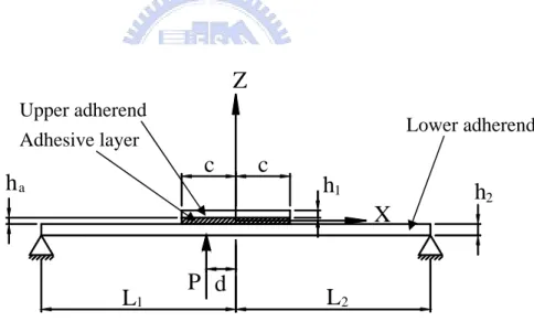
Basing on the preceding descriptions, the theoretical model is developed and the closed-form solutions also are found. In this present study both adhesively bonded adherends are subjected to a concentrated force and the peel and shear stress distributions in the adhesive layer joining the two adherends are examined as shown in Fig. 3.1. Such stress distributions are affected by geometric conditions, including the thicknesses and Young’s modulus adherends and the length, thickness, and Young’s modulus of the adhesive layer, as well as by the action point of the concentrated force. These stress distributions are investigated and the closed-form solutions are obtained by symbolic manipulation in the following sections.

Z

h

L

L

X

c

P d

c

h

1

_h

2 a 1 2 Adhesive layer Upper adherend Lower adherend

Fig. 3.1The sketch showing two adherends bonded by an adhesive layer.

3-2. Mathematical Model

In this model the two adherends – the upper adherend and lower adherend – are bonded by an adhesive layer with the center coinciding with the origin of the coordinate system. (see Fig. 3.1). The thicknesses of the upper adherend, lower adherend, and adhesive layer are denoted

by h1, h2, and ha, respectively. Their lengths are represented, respectively, by 2c, (L1+L2), and

2c. The lower adherend is subjected to a concentrated force P under the pin-pin boundary conditions.

The governing equations for this study are based on the following assumptions:

(a) The transverse displacements of both the upper adherend and of the lower adherend subjected to the concentrated force P are much smaller than their dimensions, and their transverse displacements are presumed to be linear and small.

(b) The upper adherend and the lower adherend deform under a plane-stress condition; in other words, the plane section remains plane and the deformation of the cross sections is correspondingly normal to the neutral surfaces.

(c) The variations in both longitudinal and transverse displacements are linear in the adhesive layer.

(d) In the adhesive layer, the stress resulting from the longitudinal force is ignored when compared with stresses in the upper adherend and lower adherend. [14].

Based on the preceding assumptions, the governing equations are derived as follows. First, the lower adherend is divided into four segments whose ranges are −L₁ ≤x≤−c ,

,

d x

c≤ ≤−

− −d ≤x≤c , and c≤x≤L₂ , respectively on the x-axis. Next, the upper adherend is divided into two segments whose ranges are −c≤x≤−dand on the x-axis. Finally, the adhesive layer is also divided into two segments, each of which has the same range as the corresponding segment in the upper adherend.

c x

d ≤ ≤

3-2-1. Bending moment, Shear force, and Longitudinal Force in the Upper

Adherend and Lower adherend

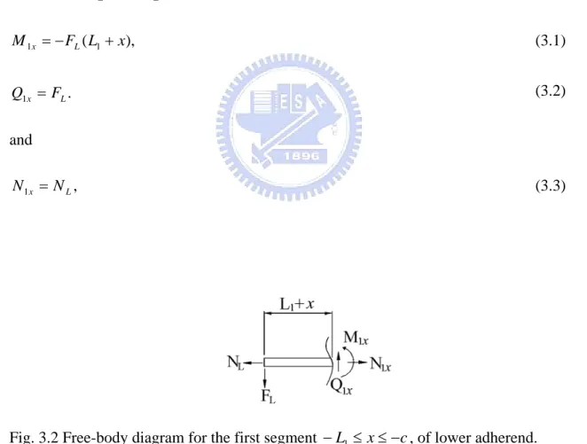
The free-body diagram for the first segment (−L₁ ≤x≤−c) is shown in Fig. 3.2– where

NL, and FL represent the longitudinal force and reaction force, respectively, of the left-end

support – and the bending moment, shear force, and longitudinal force of the first segment’s right-hand section are denoted by , and , in which the subscript refers to the first segment of the lower adherend. According to force and moment equilibrium equations, the bending moment , the shear force , and the longitudinal force can be derived in terms of , and as x x Q M1 , 1 N1x 1x x M1 Q1x N1x L N F_L : ), ( ₁ 1 F L x M _x =− _L + (3.1) . 1x FL Q = (3.2) and , 1x NL N = (3.3)

Fig. 3.2 Free-body diagram for the first segment −L₁ ≤ x≤−c, of lower adherend.

Similarly, in the free-body diagrams for the second, third, and fourth segments (displayed in Figs. 3.3, 3.4 and 3.5, respectively), the bending moment, shear force, and longitudinal

force of the section for the ith (i=2~4) segment, denoted by , and , respectively, can be written as shown below.

ix ix Q

M , N_ix

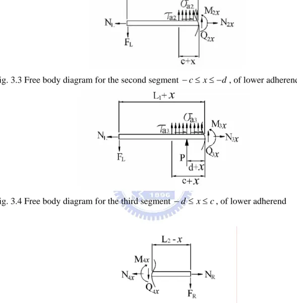
Fig. 3.3 Free body diagram for the second segment −c≤x≤−d, of lower adherend.

Fig. 3.4 Free body diagram for the third segment −d ≤ x≤c, of lower adherend

Fig. 3.5 Free body diagram for the fourth segment of c≤x≤L₂, of lower adherend.

Specifically, the bending moment, shear force, and longitudinal force of the second segment’s right-hand section (−c≤ x≤−d ) are as follows:

, 2 ) ( 2 ₂ 2 1 2

∫

∫

− − + + + − = x c x c a a L x dx h dx x x L F M σ τ (3.4)

, 2 2 F dx Q x c a L x

∫

− − = σ (3.5) and , 2 2 N dx N x c a L x

∫

− − = τ (3.6)

where σ_a2 and τ_a2 are the peel stress and shear stress for the first segment of the adhesive layer.

Similarly, the bending moment, shear force, and longitudinal force of the third segment’s right-hand section (−d ≤x≤c) are

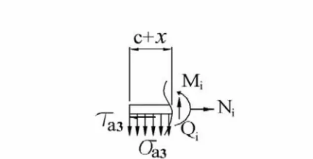
), ( 2 ) ( 2 ₃ 3 1 3 dx P d x h dx x x L F M x c x c a a L x =− + +

∫

+

∫

+ + − − τ σ (3.7) , 3 3 F dx P Q x c a L x = −

∫

− − σ (3.8) and , 3 3 N dx N x c a L x

∫

− − = τ (3.9)

where σa3 and τa3 are the peel stress and shear stress for the second segment of the adhesive

layer.

Lastly, the bending moment, shear force, and longitudinal force of the fourth segment’s left-hand section (c≤x≤L₂) are

), )( ( ) ( 2 2 4 F L x F P L x M x =− R − = L − − (3.10) ). ( 4 F F P Q x =− R = L − (3.11) and , 4x NR NL N = = (3.12)

The upper adherend, whose range is −c≤ x≤c on the x-axis, must be divided into two segments whose ranges are−c≤x≤−d and −d ≤x≤c, respectively. Free-body diagrams of these two segments are presented in Figs. 3.6 and 3.7. The bending moment, shear force, and longitudinal force of the right section of the ith segment of the upper adherend, denoted as

, and , respectively, are as follows: i i Q M , Ni

∫

∫

− − + = x c x c ai ai i dx h dx x M σ τ 2 1 _i=_{2 or 3, (3.13)} dx Q x c ai i

∫

− = σ i=2 or 3, (3.14) dx N x c ai i

∫

− = τ i=2 or 3. (3.15)

When i = 2, the range of the upper adherend is −c≤ x≤−d(i.e. the first segment of the upper adherend). However, when i = 3, the range of the upper adherend is (i.e. the second segment of the upper adherend).

c x

d ≤ ≤

−

Fig. 3.7 Free body diagram for the second segment −d≤x≤c, of upper adherend.

3-2-2. Relationship between Displacement and Stress

When the range of the adhesive layer for bonding the upper adherend to the lower adherend is −c≤ x≤c, the equations adopted from Ref. [5] are simplified by the small strain (i.e. the slope of the beam = 0) and are expressed as follows:

a ix i a ai h w w E ( − ) = σ i=2 or 3, (3.16) a h ix h i a ai h u u G _{( (} a_{) (} a₎₎ 2 2 − − = τ i=2 or 3, (3.17)

where and represent longitudinal and transverse displacements when i = 2 represents the first segment ( ) of the upper adherend and i = 3 represents its second segment ( ). In equations (3.16) – (3.17), when i = 2, transverse and longitudinal displacements for the second segment of the lower adherend are denoted by , and when i = 3, those for the third segment of the lower adherend are denoted by

These variables, which are either functions of both x and z or only a function of x, are

expressed as i u wi d x c≤ ≤− − c x d ≤ ≤ − x x u w₂ , ₂ x x u w₃ , ₃ . ), , (x z u u_i = _i u_ix =u_ix(x,z), w_i =w_i(x), and w_ix =w_ix(x) (i = 2 or 3). The longitudinal displacement (h₂a) i

) ( h₂a

ix

u − of the lower adherend are then represented as a function of x and are expressed as

either 2 a h z= or 2 a h

z=− . The symbols , and , respectively, denote the shear

modulus, Young’s modulus, and the thickness of the adhesive layer. ,

a

G E_a h_a

The stresses of the upper adhered and lower adherend are expressed as follows:

dx dui i =

σ i = 2 or 3, (3.18)

when i = 2 represents the first segment (−c≤x≤−d ) of the upper adherend and i = 3 represents its second segment (−d ≤x≤c)

The stresses of the lower adherend are expressed in

dx du_ix

ix =

σ i = 1, 2, 3, or 4, (3.19)

when i =1, 2, 3 or 4 represents the first, second, third, or forth segments of the lower adherend.

3-2-3. Relationships among Displacement, Longitudinal Force, and Bending

Moment

Following the beam theory, the transverse displacements of the upper adherend and of the lower adherend are written as shown below:

i w ix w 3 2 * 2 2 2 12 h E M dx w d ix = ix 1 or 4, (3.20) = i 3 1 * 1 2 2 12 h E M dx w d _{i i} = i=2 or 3, (3.21)

where E₂*=E , ₂ E₁*=E represent Young’s modulus of the upper adherend and of the lower ₁