錨定能對液晶盒動態響應的影響

全文

(1)國立交通大學光電工程研究所博士論文. 錨定能對液晶盒動態響應的影響 Effects of Anchoring Energy on the Dynamic Response of Liquid Crystal Cells. 研究生: 徐芝珊指導教授: 王淑霞教授梁寶芝教授. 中華民國九十四年六月.

(2) 錨定能對液晶盒動態響應的影響. Effects of Anchoring Energy on the Dynamic Response of Liquid Crystal Cells. Student: Jy-Shan Hsu. 研究生: 徐芝珊. Advisor: Prof. Shu-Hsia Chen. 指導教授: 王淑霞. Prof. Bau-Jy Liang. 梁寶芝. 國立交通大學光電工程研究所博士論文. A Dissertation Submitted to Institute of Electro-Optical Engineering National Chiao Tung University in Partial Fulfillment of the Requirements for the Degree of Doctor of Philosophy in Electro-Optical Engineering June 2005 Hsinchu, Taiwan. 中華名國九十四年六月. ii.

(3) 錨定能對液晶盒動態響應的影響研究生: 徐芝珊. 指導教授: 王淑霞教授梁寶芝教授. 國立交通大學光電工程研究所摘. 要. 液晶的動態行為在液晶元件光學反應的研究中，是一個非常基本也非常重要的課題。液晶的動態特性不僅與液晶的材料性質有關，更與液晶排列方式有著密不可分的關係。液晶的排列方式會被邊界條件所左右，其邊界條件可用錨定能密度來表示，錨定能密度則可由 easy axis 的位置與錨定能係數來決定。此外，在向列型液晶中，其指向矢的轉動與流動是互相耦合在一起的。例如：液晶指向矢的非均勻轉動會造成流動的發生，而流動亦會干擾指向矢的轉動，此效應可以在扭轉型液晶盒的光學跳躍現象與雙穩態驅動機制中發現。本論文中，我們先研究錨定能密度並用雙穩態液晶盒為例，來探討其對流動效應的影響。在錨定能密度中，預傾角是 easy axis 在極角方向的傾角。我們推導出液晶盒在外加電壓下，預傾角與相位延遲的關係，解決了測量垂直排列反射式液晶盒預傾角的問題。在測量錨定能係數時，我們發現若外加電壓使得邊界上的指向矢偏離 easy axis 變大，只考慮一項的錨定能密度函數是不合適的，此時必須加進高次項來修正。我們用包含高次項的錨定能密度模型，測量並分析二個水平排列與三個垂直排列的液晶盒所具有的錨定能係數。此外，我們以水平配向，一邊界為強錨定，另一邊界為弱錨定的雙穩態向列型液晶盒（BiNem）為例，研究在不同脈衝波的作用下，液晶盒光學表現不同的原因與機制。我們發現其弱邊界上的指向矢，在脈衝波作用結束時的位置，會影響後來的液晶動態行為。最後，我們設計並做出一種新的雙穩態液晶顯示模態（BHN）的液晶盒，藉由液晶的流動效應與雙頻液晶的特性，構成轉換機制。在實驗上，其切換電壓僅需為 5 V 即可達成穩態間的轉換。 i.

(4) Effects of Anchoring Energy on the Dynamic Response of Liquid Crystal Cells. Student: Jy-Shan Hsu. Advisors: Prof. Shu-Hsia Chen Prof. Bau-Jy Liang. Institute of Electro-Optical Engineering National Chiao Tung University. Abstract Consider as an important subject for the study of the electro-optical response in the liquid crystal (LC) device, the dynamic behaviors of liquid crystals are not only related to the intrinsic properties of the LC material itself but also to the spatial orientation of the LC directors.. The arrangement of the directors in a cell is controlled by the boundary. conditions, which can be described by the anchoring energy density determined by the position of the easy axis and the coefficients of the anchoring energy density.. Moreover,. there is a coupling between the translational motion and the rotational motion of the nematic LC directors. For example, the non-uniform rotations of LC directors induce the shear flow of the LC director; conversely, the shear flow disturbs the orientation of the LC directors. The shear flow effect can be observed in the optical bounce of twisted nematic cells and some of the switching mechanisms of bistable devices. In this research, we first studied the anchoring energy density and than used two bistable cells as examples to investigate the impact of the shear flow effect.. Within the. anchoring energy density, the pretilt angle is the tilt angle of the easy axis in the polar direction. We derived the relationship between the pretilt angle and the phase retardation as a function of applied electric field and solved the problem of obtaining the pretilt angle ii.

(5) of a non-twisted, vertical aligned reflective cell. When measuring the anchoring energy coefficients, we found the higher order terms of the anchoring energy density cannot be negligible when the applied voltage becomes large.. By using the anchoring energy. density with one higher order term, we measured the anchoring energy coefficients of two homogeneous cells and three homeotropic cells. Furthermore, we investigated the optical response of Bistable nematic (BiNem, a homogeneous aligned cell with one weak anchoring substrate and one hard anchoring substrate) cell by applying voltage pulses with various durations. We found that the position of the weak-boundary director at the end of the pulse has a crucial impact on the relaxation behaviors.. Finally, we designed and demonstrated a novel bistable mode,. namely, the bistable chiral-tilted homeotropic nematic (BHN) LC device.. The switching. mechanism is achieved by the shear flow effect and the anisotropic properties of a dual frequency liquid crystal.. The experimental switching voltage of the device is only 5 V.. iii.

(6) 致謝首先感謝我最親愛的父母親：徐元錫先生及朱鏡如女士，謝謝他們給予我最大的支持與鼓勵，沒有他們就沒有今天的我。感謝我的公公與婆婆：黃金玉先生及黃胡火珠女士的照顧，細心地呵護黃潔和宇冬，讓我無後顧之憂的完成博士學程。此外也要感謝大姊芝倫、二姊芝敏、妹妹夢蘭、大伯文淦、大嫂美雲、大姑秀梅與小姑錦鈴的支持與關心。特別感謝指導教授王淑霞老師在學術研究與為人處事上的諄諄教誨，使我在知識與生活上受益良多。指導教授梁寶芝老師在心靈與生活上的引領，耐心的與我討論研究上的盲點。兩位指導老師使我順利地以嚴謹而且踏實步伐完成此研究及論文。感謝學長陳立宜博士、楊秋蓮博士與謝志勇博士在理論模擬方面的幫助。感謝俊雄、范姜、怡安帶著我一同準備資格考，那一段一起唸書，討論與打 AOC 以紓解壓力的日子，令人難忘。感謝美琪、品發、家榮陪我一起做實驗，並還幫我收實驗數據，一起討論與分析實驗上所碰到的問題。感謝孩子們黃潔和宇冬，他們的支持與笑容一直是我心中最大的快樂與支柱。感謝實驗室的學長姐及學弟妹: 秋蓮、志勇、阿寬、俊雄、范姜、怡安、揚宜、彥廷、信全、乾煌、梓傑、佳成、惠雯、庭瑞、朝旭、英豪、舒展、德源、建宏、世郁、品發、美琪、家榮、庭毅、瑞傑陪我一起走過酸甜苦辣的博士班生活，我們在實驗室的互動為平淡的生活帶來不少的樂趣與歡笑。最後這年，更要感謝范姜、庭毅、瑞傑一起分擔實驗室的工作，並能相互扶持一同畢業。僅以此論文獻給我最親愛的父母、公婆、孩子們、以及所有關心我和幫助過我的人，謝謝你們。. 徐芝珊新竹交通大學 2005 年 5 月 iv.

(7) Contents 摘要 ....................................................................................................................i Abstract ............................................................................................................ ii 致謝 .................................................................................................................. iv Contents ............................................................................................................v List of Figures.................................................................................................. vii List of Symbols ................................................................................................. xi Chapter 1 Introduction ..................................................................................... 1 1.1 The meaning of the anchoring energy ................................................. 1 1.2 The dynamic response of liquid crystal cell ......................................... 2 1.2.1 For the cells with strong anchoring............................................... 3 1.2.2 For the cell with weak anchoring .................................................. 5 1.3 Aims of the research ............................................................................ 6 Chapter 2 Theory........................................................................................... 10 2.1 The continuum theory for nematic liquid crystal ................................ 10 2.1.1 Theory of elasticity: Oseen-Zöcher-Frank theory....................... 10 2.1.2 Hydrodynamic theory: Ericksen-Leslie theory............................ 13 2.2 Models of the anchoring energy density ............................................ 19 2.2.1 Rapani-Popular model................................................................ 20 2.2.2 Other models.............................................................................. 20 Chapter 3 Study on the anchoring energy density ........................................ 28 3.1 Determination of the pretilt angle of the reflective liquid crystal cells 29 3.1.1 Theory ........................................................................................ 29 3.1.2 Experimental results and comparisons ...................................... 34 3.1.3 Conclusion.................................................................................. 37 3.2 Determination of the higher order polar anchoring coefficients ......... 38 3.2.1 Theory ........................................................................................ 38 3.2.2 Experiment ................................................................................. 41 v.

(8) 3.2.3 Discussion and Conclusion ........................................................ 43 Chapter 4 Bistable nematic liquid crystal cells (BiNem) ................................ 47 4.1 Introduction ........................................................................................ 47 4.2 Dynamic behaviors induced by pulses with different durations ......... 48 4.3 Analysis.............................................................................................. 50 4.4 Relation between polar anchoring energy coefficients and voltage of the switching pulses....................................................................... 54 Chapter 5 Bistable chiral-tilted homeotropic nematic (BHN) liquid crystal cell................................................................................................. 59 5.1 Introduction ........................................................................................ 59 5.2 Theory................................................................................................ 60 5.3 Experimental results .......................................................................... 62 Chapter 6 Summery and future scope........................................................... 66 Vita ................................................................................................................ 68. vi.

(9) List of Figures Figure 1.1. Sketch of geometry for the easy axis and the deviation angle……………….. 2. Figure 1.2. (a) The director configuration of a twisted nematic cell under normally black mode before and after the switching off process. (b) The calculated transient intensity without considering the flow effect.. (c) The optical bounce can. be found in the transient intensity after turning off the applied voltage in the experimental data.…………………….…………………..………………..... 3 Figure 1.3. (a) The director configuration of a quasi-homeotropic cell before and after the switching on process. (b) The calculated transient intensity without considering the flow effect. (c) The optical bounce can be found in the transient intensity after turning on the applied voltage in the experimental data...………..……………………………………………..…………………. 4. Figure 1.4. The configurations of the BiNem cell: (a) Uniform state (U state), (b) Deformed state (D state), (c) Twisted state (T state). U state and T state are the stable states at V=0V and (b) is under an applied voltage. (d) ~ (g) show that the fast switching off the field creates a strong shear flow and the cell relaxes to the T state. (h) and (i): show that the slowly switching off the field does not induce enough shear flow and the cell goes back to the U state…...........................................................................................................… 7. Figure 2.1. Sketch of the geometry and the coordinates for a free director under an applied electric field. The induced torque is related to the angle between the director and the direction of the electric field………………………….. 12. Figure 2.2. The liquid crystal cell, which has infinite extension in the x and y directions, is bounded at z = 0 and z = d. The layer is divided into m equally spaced sub-layers. Fluid velocities and director orientation are functions of z and t only…………………………………………………………………………. 16. Figure 2.3. The liquid crystal director under an external electric field.. The director. rotates by the electric field and induces the movement of the center of mass of the director.. The movement of the director will influence the rotation of. the director…………………………………………………………………… 18 Figure 2.4. The interfacial potential of Rapani-Papoular model………………………... vii. 20.

(10) Figure 2.5. 1 2. 1 2. The interfacial potential of f s = Wθ sin2 (α − αe ) + Wφ sin2 (φ − φe ) with αe=45°,. φe=0°, Wθ =1, Wφ =0.5 (a), (d) and (b), (e) are the polar and azimuthal anchoring energy portions of fs, respectively. The third column is the combination of these two energies. The height in the first row and the colors in the second row represent the values of anchoring energy…………. 21 Figure 2.6. 1 2. 1 2. The interfacial potential of f s = Wθ sin2 (α − αe ) + Wφ sin2 (φ − φe ) with αe=45°,. φe=0°, Wθ =1, Wφ =0.5……………………………………………………… 22 1 2. 1 2. 2 2 2 Figure 2.7 The interfacial potential of f s = Wθ sin (α − αe ) + Wφ sin (φ − φe ) cos α with αe=0°,. φe=0°, Wθ =1, Wφ = 0.5……………………………………………………… 22 Figure 2.8. 1 2. 1 2. The interfacial potential of f s = Wθ sin2 (α − αe ) + Wφ sin2 (φ − φe ) cos2α with. αe=45°, φe=0°, Wθ =1, Wφ = 0.5…………………………………………….. 23 Figure 2.9. The surface anchoring energy of the unified model as the pretilt decrease from 90° (a) to 45°(c), 25°(f), and 0°(h)…………………………………… 24. Figure 2.10 ξˆ (ηˆ ) is the angle between the nodal line and y-axis, ξˆ (ηˆ ) is the angle between the nodal line and h-axis………………………………………….. 25 Figure 2.11 The surface anchoring energy of the unified model as the pretilt decrease from (a) to 60°(c), 25°(f), and 0°(h)………………………………………... 26 Figure 3.1. The phase retardations obtained from the simulated director profiles for pre-polar angle from 1° to 7°: (a) with respect to the applied voltage, (b) with respect to the inverse of the applied voltage, (c) with respect to the square of the applied voltage. The linearly fitting curves are plotted in dash lines for each pre-polar angles……………………………………………... 33. Figure 3.2. The optical setup used for measuring the phase retardation of a reflective VA-LC cell…………………………………………………………………. 35. Figure 3.3. The measured phase retardation of the VA reflective cell: (a) with respect to the applied voltage, (b) with respect to the inverse of the applied voltage, (c) with respect to the square of the applied voltage. The solid lines in (b) and (c) are the linearly fitting curves to get the cell gap and the pre-polar angle, respectively………………………………………………………….. 36. Figure 3.4. Sketch of geometry and coordinates for a homogeneous nematic layer deformed by an applied field……………………………………………….. 39. Figure 3.5. The setup for measuring the phase retardation as a function of applied voltage…………………………………………………………….………... 42 viii.

(11) Figure 3.6. The measured δ−V curve together with a series of δ−V curves simulated with different Wθ,RP of a homogeneous cell. The left inset shows the small applied voltage regime in which the experimental δ−V curve agrees well with one of the simulated curves. The right inset shows δ−V curves in the large applied voltage regime in which the experimental curve is intercepted with simulated curves of different Wθ,RP………………………. 42. Figure 3.7 The anchoring energy versus the deviation angle of (a) a homogeneous cell, (b) a homeotropic cell……………………………………………………… 45 Figure. 4.1 The textures and the transitions of the BiNem cell………………………… 48 Figure 4.2. The dynamic trajectories of the directors in the normal-twisted relaxation process (a) and the optical response (b) when the cell was switched form U state to T state by applying a 2 ms pulse of 13V…………………………… 51. Figure 4.3. The dynamic trajectories of the directors in the over-twisted relaxation process (a) and the optical response (b) when the cell was switched form U state to T state by applying a 1 ms pulse of 13V…………………………… 51. Figure 4.4. The dynamic tilt and azimuthal angles of nrb when we applying pulses of 13V with different duration: (a) 2 ms (b) 1 ms and (c) 0.5 ms.. The tilt. and azimuthal angles of nrb in the normal-twisted relaxation process and the over-twisted relaxation process are shown in (a) and (b), respectively. When the pulse is too short which is the case of (c), the cell is not switched to the T state and relaxes to the U state…………………………………….. 53 Figure 4.5. The critical voltage (square) and the minimum required voltage (triangle) as function of the polar anchoring energy coefficient for switching the cell from the U state to the T state. The pulses with higher applied voltages can be used to switch the cell to the T state and with the lower voltages make the cell remain in the U state……………………………………………….. 56. Figure 4.6. The minimum required voltage as function of the polar anchoring energy coefficient for switching the cell from the U state to the T state by using a 1ms pulse (triangle) and the 2 ms pulse (square). The pulses with higher applied voltages can be used to switch the cell to the T state and with the lower voltages make the cell remain in the U state………………………… 57. Figure 5.1. Bistable textures and transition processes of the BHN device…………….. 61. Figure 5.2. The transient transmittance and the corresponding driving waveform of the ix.

(12) BHN device switched from the T state to the TH state. The amplitude of the driving pulse is 5 volts and the frequency is 1 kHz…………………….. Figure 5.3. 63. The transient transmittance and the corresponding driving waveform of the BHN device switched from the TH state to the T state. The amplitude of the driving pulse is 5 volts. The frequency is switched from 1 kHz to 100 kHz…………………………………………………………………………… 63. Figure 5.4. Transmission micrographs of the BHN device under the crossed-polarizer condition. (a) The tiltedly homeotropic state; (b) the biased homeotropic state; (c) the twisted state; (d) the biased twisted state……………………..... 64. List of Tables Table 3-I. Parameters used in the simulation………………………………………….... Table 3-II. The pre-polar angles obtain in the Figure 3.1(c) with different fitting ranges. 32. of the square of the applied voltage. The upper limit of the applied voltage is V upper and θ0s and θ0e are the pre-polar angles used in the simulation and calculated from the slopes in Figure 3.1(c), respectively..…………………... 34. Table 3-III The determined Wθ , ζ and the corresponding alignment materials, the methods, cells parameters……………………………………………………. 44 Table 4-I. The cell and liquid crystal material parameters used in the simulation……... 49. Table 4-II. The cell parameters used in the simulation………………………………….. 55. x.

(13) List of Symbols r D r E. applied electrical field. Ftotal. total free energy of the cell. Gi. external director body force per unit volume. V. applied voltage. Vth. threshold voltage. d. cell gap. fbulk. Frank free energy density. felec. electric free energy density. fi. fluid body force per unit volume in i direction. fs. surface free energy density or anchoring energy density. ftotal. total free energy per unit area. gi. intrinsic director body force per unit volume in the i direction. g i0. static (elastic) part of intrinsic director body force per unit volume in the i. applied displacement. direction. g 'i. hydrodynamic (viscous) part of intrinsic director body force per unit volume in the i direction. k11. splay elastic constant. k22. twist elastic constant. k33. bend elastic constant. r n. director orientation. ne. extraordinary refraction index of liquid crystal. no. ordinary refraction index of liquid crystal. q0. q0=2π/p, p: pitch of colesteric structure. t ji. fluid stress tensor. t 0ji. elastic part of fluid stress tensor xi.

(14) t' ji. hydrodynamic part of fluid stress tensor. vi. fluid flow velocity. ∆ε. dielectric anisotropy of liquid crystal. ∆n. refractive anisotropy of liquid crystal. Γ ,δ. phase retardation. α. tilt angle of director. α0. pretilt angle. αs. tilt angle of surface director. α1~α6. Leslie viscosity coefficients. ε //. dielectric constant parallel to the director of liquid crystal. ε⊥. dielectric constant perpendicular to the director of the liquid crystal. φ. azimuthal angle of director. γ. Largrange multiplier. γ1. rotational viscosity coefficient, γ1=α3−α2. γ2. viscosity coefficient, γ2=α6−α5. η 1~ η 3. shear viscosity coefficients. λ. wavelength of light. πji. director surface stress tensor. θ. polar angle of director. ρ. mass density of fluid. ρ1. moment of inertia. τi. viscous torque. τE. electric torque. xii.

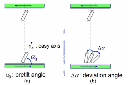
(15) Chapter 1 Introduction The electro-optical characteristic of a liquid crystal (LC) cell is determined by the bulk behaviors of the molecules. The configuration of LC molecules is, in turn, determined by the arrangement of the LC molecules on the boundary which is controlled by the alignment layer. There are several parameters used to describe the properties of the interface between the LC and alignment layer, such as the coordinates of the easy axis as well as the anchoring energy coefficients. The former describe the minimum position of the interfacial surface free energy and the later determine the abilities of the LC molecules to deviate from the easy axis. On the other hand, in order to improve the performance of the liquid crystal display (LCD), the dynamic behaviors of the LC molecules need to be investigated. The shear flow effect, which is sometimes ignored in the LCD design, can affect the optical response of the LCD. In this chapter, we briefly describe these effects with different boundary conditions.. 1.1 The meaning of the anchoring energy The interaction between the LC molecules and the alignment layer is subtle. From the macroscopic view, we adopt the surface free energy density (anchoring energy density) to describe the characteristic interface interaction.. Without any external force, the LC. molecules on the boundary are aligned in the easy axis, as shown in Figure 1.1 (a), which orient in the minimum state of the surface free energy density. When there are external forces acting on the LC molecules, the boundary director deviates from the easy axis, which is shown in Figure 1.1 (b). To describe the surface effect, Rapini and Papoular(1) introduced a simple phenomenological expression for the interfacial surface free energy per unit area, fs, which describes the interaction between the nematic LC director and the substrate of homeotropic 1.

(16) 1 anchoring: f s = W sin 2 (θ ) , where θ is the polar angle of the director and W is the 2. anchoring energy coefficient. The larger the W, the harder the director can be deviated from easy axis, which is the strong anchoring boundary condition.. Small W means weak. anchoring boundary condition. After Rapini-Papoular’s (R-P) work, many attempts have been made to generalize the RP model in order to describe the planar and tilt anchoring properties. The anchoring energy coefficients of a planar surface direction are the azimuthal anchoring energy coefficient Wφ, which is related to the deviations from the easy axis in the azimuthal direction, and the polar anchoring coefficient Wθ, which is corresponding to the deviations from the easy axis in the polar direction.. (a). (b). Figure 1.1 Sketch of geometry for the easy axis and the deviation angle.. 1.2 The dynamic response of liquid crystal cell The dynamical behavior (2,3) of liquid crystal displays (LCDs) is not only related to the LC materials but also to the boundary parameters. Due to the complication of the dynamical problem which is associated with five nonlinear coupling equations of the director and flow velocity, it is difficult to deduce the analytic form. Usually, the flow effect of liquid crystals and the boundary conditions are simplified by considering only the rotational viscosity and rigid boundary condition, respectively.. Under the pure rotational model with rigid. boundaries, only a time constant is used to characterize the response time of the LC devices, which is derived through the equation of motion of the director balanced between the 2.

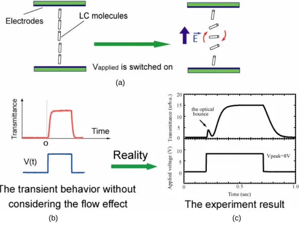
(17) rotational viscous, elastic and electric torques. However, without the consideration of shear flow effect and the boundary condition carefully, the dynamical behavior of the LC devices can not be predicted accurately.. (a). (b). (c). Figure 1.2 (a) The director configuration of a twisted nematic cell under normally black mode before and after the switching off process. (b) The calculated transient intensity without considering the flow effect. (c) The optical bounce can be found in the transient intensity after turning off the applied voltage in the experimental data.. 1.2.1 For cells with strong anchoring Usually the LC boundary directors are regarded as they are rigidly anchored on the substrates, although, it is never true for the boundary directors. It is a good approximation for the rubbed polyimide (PI) alignment layers. From the reported literature, the measured polar and azimuthal anchoring energy coefficients of the rubbed PI are around 10−3 J/m2 and 10−4 J/m2, respectively, which makes the behaviors of the LC directors closed to that of the rigid boundary condition. Figure 1.2 shows a twisted nematic (TN) LC cell being switched off from a high field. 3.

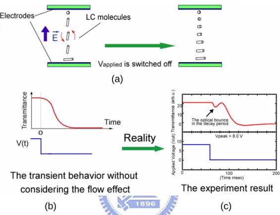
(18) The transient behaviors, which do not include the shear flow effect, are different from the experimental results.. Figures 1.2 (b) and (c) illustrate an optical bounce in the decay. process of the experimental result while there is not in the simulation when the shear flow effect is not included. The dynamical behaviors, which exist in the TN-mode LC device have been studied more than 20 years since van Doorn (4) and Berreman (5) independently showed that the importance of hydrodynamic flow in the transient behavior of liquid crystals. The optical bounce in the decay process originates from the flow-induced tipped-over and reverse twist effect of liquid crystals. In addition to the decay process, the shear flow effect influences the director orientation in the rising process. Though, there are no significant effects on the optical response.. (a). (b). (c). Figure 1.3 (a) The director configuration of a quasi-homeotropic nematic cell before and after the switching on process. (b) The calculated transient intensity without considering the flow effect. (c) The optical bounce can be found in the transient intensity after turning on the applied voltage in the experimental data.. The shear flow effect can also be observed in the transient behavior when a quasi-homeotropic cell is switched to a high field. (6-12). . Figure 1.3 (a) shows the director. configuration of a quasi-homeotropic nematic LC cell being switched on to a high field. Figure 1.3 (b) shows when the flow effect is not included, the simulated optical response of 4.

(19) the switch on process rises smoothly. experimental result.. However, Figure 1.3 (c) shows a bump in the. The detailed switching mechanisms have been studied by Dr. Chen (6-9). and Dr. Hsieh (10-12) of our group and the reasons causes of the optical bounce are the shear flow and the asymmetry of the boundary (11). These two examples illustrate the varied results of the shear flow effect on the transient behaviors of TN and quasi-homeotropic cells with hard anchoring boundary. Since the alignments of the boundaries in the cells are different, the configurations of the directors are different; the effects of the shear flow are distinct and need to be studied carefully.. 1.2.2 For cells with weak anchoring In addition to the rubbed PI, there are many ways to align LC molecules on the substrates, e.g. SiOx sputtering, photo-alignment, atomic-beam alignment, atomic force microscope scan method.. Since the interfacial anchoring properties of these alignment. methods vary from hard to weak, one should not regard the boundary directors as they are rigidly anchored on the substrates. Recently, the photo-alignment materials are getting more stable and popular in the application of LCDs.. For better understanding the behaviors of the. displays, we should include the surface free energy density in the modeling of LCD. In general, when a small field is applied to a LC cell, the shear flow effect is small and can be ignored. The directors simply rotate toward the direction of the field. Since the directors on the boundaries can be rotated easier for the weaker anchored directors, the cell moves to the final on state faster.. Therefore, the response time of weakly anchored. boundary directors is less than that of the hard anchored boundary directors. However, when the field is tuned off, the final state is determined by the relaxation process. The weakly anchored directors have less surface torque to rotate themselves back to the easy axis. The response time is, therefore, longer due to the relaxation time required for the boundary directors back to the final position. When a high field is suddenly applied upon or removed from a cell, one cannot ignore the shear flow effect. As show in Figure 1.2 and 1.3, the shear flow effect influences the transient behavior of the LC directors with hard boundary condition and can be seen from the optical response. What is the outcome when the boundary directors of the cell are weakly anchored on the substrates? A typical application of the weak anchoring boundary is the bistable nematic liquid crystal cell (BiNem) proposed by Dozov (13,14) et al. in 1997. It has many superior properties, 5.

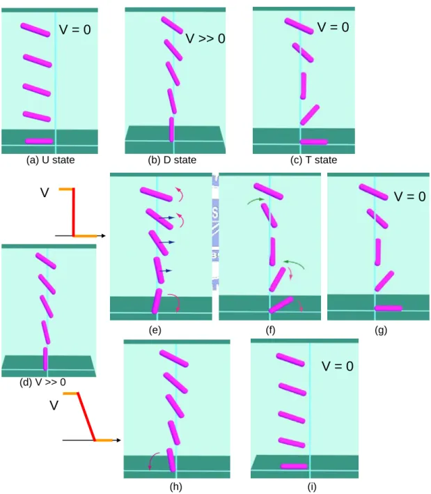
(20) such as simple structure, fast response, high contrast ratio and wide viewing angle in addition to the permanent memory effect. The two stable states, of which the twisted angles differ by. π as shown in Figures 1.4(a) and (c), can be switched through the shear flow effects and polar anchoring energy breaking on one substrate. According to the papers of Dozov, the two stable states of the BiNem cell are the U state and the T state. The upper substrate is treated to have strong polar anchoring energy with high pretilt angle, and the bottom substrate has weak polar anchoring energy and the pretilt angle is nearly zero. If the field is larger than the critical electric field, which is defined as the anchoring energy breaking of the bottom substrate, the directors near the bottom substrate are vertical, which is the D state and shown in Figure 1.4 (b). After the field is removed, the directors relax to either one of the bistable states. From the theory proposed by Dozov, the final state selection is determined by the flow effect induced by the pulse. Fast switching off the field creates a strong shear flow and the cell relaxes to the T state (Figure 1.4 (d) ~ (g)). Slowly switching off the field does not induce enough shear flow and the cell goes back to the U state (Figure 1.4 (d), (h) and (i)). This example shows the application of the shear flow effect with weak anchoring boundary.. 1.3 Aims of this research Rencently, our group has done many investigations on the dynamical behavior for different LCD modes. Dr. Li-Yi Chen (6-9) explored the influence of the flow effect on the dynamical behavior of homeotropic-like LC cells.. He found that the optical-bounce. phenomenon, which was originally discovered in the TN-LC cell, also appears in the rising period of the chiral-hoemotropic and pure homeotropic liquid crystal cells. The optical-bounce behavior is caused by the flow-induced twist deformation. He proposed that the response time of the homeotropic-like cell can be improved by a larger twist elastic constant. Furthermore, based on the observation of the transient transmittance of the pure homeotropic cell, he predicted the existence of two stable states in the homeotropic liquid crystal cell and demonstrated a new bistable liquid crystal device which can operate between three states. Afterward, Dr. Chih-Yung Hsieh (10-12) explored the boundary effects on the dynamical behavior of three classes of liquid crystal cells whose boundary directors are not precisely normal to the substrates: the quasi-homeotropic liquid crystal (QHLC) cell, the bistable chiral QHLC cell and π/2 bistable chiral QHLC cell.. The optical oscillation. (double-bounce phenomenon) in the QHLC cells during the rising period originates from not only the flow effect of liquid crystals but also the complicated alignment condition, which is 6.

(21) a combination of the deviation and azimuthal alignment and the asymmetrical polar alignment.. The flow effect of liquid crystals and the asymmetrical polar alignment. condition are important factors to achieve the switching bistabiliy of the bistable chiral QHLC cell.. Hsieh also presented an electric switching π/2 bistable chiral QHLC cell with. low driving voltage (12).. V=0. (a) U state. V=0. V >> 0. (b) D state. (c) T state. V. V=0. (e). (f). (g). V=0 (d) V >> 0. V. (h) Figure 1.4. (i). The configurations of the BiNem cell: (a) Uniform state (U state), (b) Deformed state (D state), (c). Twisted state (T state).. U state and T state are the stable states at V = 0V and (b) is under an applied voltage.. (d) – (g) show that the fast switching off the field creates a strong shear flow and the cell relaxes to the T state. (h) and (i) show that the slowly switching off the field does not induce enough shear flow and the cell goes back to the U state. 7.

(22) In this dissertation, we consider the boundary directors to be non-rigidly anchored on the substrates. The interfacial potential between the boundary directors and the alignment layer is called the surface free energy density, or the anchoring energy density. For simplicity, it can be determined by the coordinate of the easy axis (the minimum of the surface free energy density) and the anchoring energy coefficients.. In Chapter 2, we first review the. nemato-hydrodynamic theory and the models of the anchoring energy density. In Chapter 3, we investigate and propose methods to measure the interfacial parameters including the pretilt angle of the easy axis in the reflective vertically aligned (VA) LCD and the anchoring energy coefficients of homogeneous and homeotropic cells. After that, we combine the shear flow effect and the non-rigid boundary condition. In Chapter 4, we study the BiNem cell by adopting the weak anchoring in one of the substrates and using flow effect to achieve the switching.. Several distinct dynamic behaviors appear. The mechanisms of these. behaviors are explicitly explained through the tilt and azimuthal angles of the surface director on the weak anchoring boundary in the dynamic process. In Chapter 5, we propose a bistable mode—bistable chiral-tilted homeotropic nematic LC cell, BHN. The two stable states are the tilted homeotropic state and the twisted state.. The main switching. mechanisms are achieved by the shear flow effect together with the anisotropic properties of the dual-frequency LC material. Finally, in Chapter 6, a summary and future scopes are made.. 8.

(23) References of Chapter 1 1. A. Rapini and M. Papoular, J. Phys. (Paris) Colloq., 30, C4-54, (1969).. 2. P. G. de Gennes and J. Prost, The Physics of Liquid Crystals. Clarendon Press, second edition, 1993.. 3. S. Chandrasekhar. Liquid Crystals. Cambridge University Press, second edition, 1992.. 4. C. Z. van Doorn., J. Appl. Phys., 46, 3738, (1975).. 5. D. W. Berreman,. J. Appl. Phys., 46, 3746, (1975).. 6. Shu-Hsia Chen and Li-Yi Chen, Appl. Phys. Lett., 75, 3491, (1999).. 7. L.Y. Chen and S.H. Chen, J. SID, 7, 289, (1999).. 8. Li-Yi Chen and Shu-Hsia Chen, Jpn. J. Appl. Phys., 39, L368, (2000).. 9. Chih-Yung Hsieh and Shu-Hsia Chen, Jpn. J. Appl. Phys., 41, 5264, (2002).. 10. Li-Yi Chen and Shu-Hsia Chen, Appl. Phys. Lett., 74, 3779, (1999).. 11. Chih-Yung Hsieh and Shu-Hsia Chen, Appl. Phys. Lett., 83, 1110, (2003).. 12. Chih-Yung Hsieh and Shu-Hsia Chen, Jpn. J. Appl. Phys., 42, L1330, (2003).. 13. I. Dozov, M. Nobili, and G. Durand, Appl. Phys. Lett., 70, 1179, (1997).. 14. I. Dozov and G. Durand, Liquid Crystals Today, 8, 2, (1998).. 9.

(24) Chapter 2 Theory In this chapter, we will discuss the theory of the dynamic behavior of nematic liquid crystals and the anchoring properties of LC directors on the boundary. First, we will give a brief review of the theory of elasticity (1,2), which is used to characterize the static spatial director field, and nemato-hydrodynamic theory (3,4), which is applied to deal with the fluid motion of nematic liquid crystals. Then, we study the anchoring properties of the boundary and introduce several models of the anchoring energy density proposed in the literatures.. 2.1 The continuum theory for nematic liquid crystal Rigid rods are the simplest type of objects used to describe nematic LC molecules behaviors. The average direction of the alignment of certain amount molecules is along one r r r r common direction, which is called director ( n ). It is uniaxial with n = 1 and n = − n .. r. The continuum theory for the nematic liquid crystal is under the assumption that n varies slowly and smoothly with respect to the position.. We applied this theory to investigate the. static and dynamical behavior of nematic liquid crystals under external optical, electric or magnetic fields.. 2.1.1 Theory of Elasticity: Oseen-Zöcher-Frank theory For an incompressible fluid and an isothermal deformation of the nematic liquid crystals, the total elastic free energy (Ftotal) of the system can be written as: Ftotal = ∫ f bulk dV + ∫ f surface dS V. 10. (2.1).

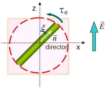
(25) where fbulk is the elastic free energy per unit volume and fsurface is the surface free energy per unit area. In this section, we only focus at the bulk liquid crystals. The elastic free energy density of the deformed nematic liquid crystals can be written as: 1 v v v v v f bulk = [k11 (∇ ⋅ n ) 2 + k22 ( n ⋅ ∇ × n + q0 ) 2 + k33 ( n × ∇ × n ) 2 ] 2. (2.2). where k11, k22 and k33 are the splay, twist and bend elastic constants, respectively. q0 is 2π/p, where p is the pitch of the helix. For an untwisted nematic liquid crystals, q0 is equal to 0, the pitch of the helix approaches to infinity (p = ∞).. Equation (2.1) is derived from. considering the curvature strains of the director. Other types of deformation either do not change the elastic free energy or are forbidden due to the symmetry of the liquid crystals and the absence of polarity (head to tail symmetry). It also neglect higher order terms because only the small deformations are considered. That is, only the quadratic terms are included in the elastic free energy density which resembles to the Hook’s law.. LC Directors in the Electric Field Let’s consider the dielectric interaction between a nematic LC director and the electric r r field. For an applied electric field (DC or low-frequency) E , the displacement D may be rewritten as: r r v v r D = ε 0ε ⊥ E + ε 0 (ε // − ε ⊥ )(n ⋅ E )n .. (2.3). 1 r r 1 1 v v f elec = − D ⋅ E = − ε 0ε ⊥ E 2 − ε 0 ∆ε (n ⋅ E ) 2 . 2 2 2. (2.4). The electric energy density is. Note that the first term on the right-hand side of Eq. (2.4) is independent of the orientation of the director axis. Therefore, the electric torque acting on the LC directors is r. r. r ⎛ ∂f elec ⎞ v v r r r ⎟ = ε 0 ∆ε (n ⋅ E )( n × E ) ⎝ ∂n ⎠. τ E = n × fE = n × ⎜ −. 1 = ε 0 ∆εE 2 sin(2ξ ). 2 11. (2.5).

(26) where ξ is the angle between the director and the electric field shown in Figure 2.1. When the director is free to rotate, the torque is maximum when the angle between the director and the direction of the electric field is 45°.. τe. z. ξ. r n director. Figure 2.1. r E x. Sketch of the geometry and the coordinates for a free director under an applied electric field.. The induced torque is related to the angle between the director and the direction of the electric field.. Euler-Lagrange equation for a LC system under the external applied field. r Let’s consider a nematic liquid crystal slab of thickness d in an external electric field E .. For simplicity, we have supposed that all variable depend only on the z-coordinate, the total free energy per unit area of the system is given by f total [ ϕ ( z )] = ∫. d /2 −d / 2. f bulk [ ϕ ( z ), ϕ ' ( z ); z ] dz + f s1 (ϕ1 ) + f s 2 (ϕ 2 ) .. (2.6). where ϕ characterizes the deformation, and ϕ ' = dϕ dz . fbulk is the bulk elastic free energy density and fs1(ϕ1) and fs2(ϕ2) the surface energy density, with ϕ1 = ϕ ( − d 2) , ϕ 2 = ϕ ( d 2) . If ϕ~ ( z ) is the function minimizing the function ftotal[ϕ (z)]. ϕ (z) is chosen to close to. ϕ~ ( z ) , in the following way ϕ ( z ) = ϕ~( z ) + αυ ( z ) , where υ (z) ∈ C 1 is an arbitrary function and α a small parameter.. 12.

(27) ⎧ d ⎡ df total ⎤ ⎢⎣ dα ⎥⎦ = ⎨⎩ dα α =0. ∫. d 2 −d 2. f bulk [ϕ ( z ), ϕ ' ( z ); z ] +. df s1 (ϕ1 ) df s 2 (ϕ 2 ) ⎫ + ⎬ , dα dα ⎭α =0. df bulk ∂f bulk ∂ϕ ∂f bulk ∂ϕ ' = + dα ∂ϕ ∂α ∂ϕ ' ∂α where ⎤ ⎡ d ∂f bulk ⎤ d ⎡ ∂f ∂f bulk υ ' = ⎢ bulk υ ⎥ − ⎢ υ dz ⎣ ∂ϕ ' ⎦ ⎣ dz ∂ϕ ' ⎥⎦ ∂ϕ ' ⎧⎪ ⎡⎛ ∂f ⎫ ⎧ d 2 ⎡ ∂f bulk d ∂f bulk ⎤ ⎡ df total ⎤ bulk + − = υ ( ) z dz ⎬ ⎨ ⎨ ⎢⎜⎜ ⎥ ∫ ⎢⎣ dα ⎥⎦ − d 2 ⎢ ∂ϕ ∂ ∂ dz ϕ ϕ ' ' ⎣ ⎦ α =0 ⎭α =0 ⎪⎩ ⎣⎢⎝ ⎩. ⎫⎪ ⎞ df ⎤ ⎟⎟ + s 2 ⎥ υ ( d 2) ⎬ ⎠ d 2 dϕ 2 ⎦⎥ ⎪⎭α =0. ⎧⎪ ⎡⎛ ∂f ⎞ ⎫⎪ df ⎤ + ⎨ ⎢⎜⎜ bulk ⎟⎟ + s1 ⎥ υ ( − d 2 ) ⎬ ⎪⎩ ⎢⎣⎝ ∂ϕ ' ⎠ −d 2 dϕ1 ⎥⎦ ⎪⎭α =0. (2.7). Since ϕ~( z ) minimizes ftotal, we deduce that. ⎡ df. ⎤. δ f total = ⎢ total ⎥ α = 0 , ⎣ dα ⎦α =0. ∀ υ (z) ∈ C 1 ,. Consequently, from Eq. (2.7), It follows that ϕ~( z ) is the solution of the Euler-Lagrange equation:. ∂f bulk d ∂f bulk − = 0, ∂ϕ~ dz ∂ϕ~'. ∀z ∈ ( − d 2 , d 2).. (2.8). And satisfies the boundary conditions. −. ∂f df ∂f bulk df s1 + = 0, − bulk + s 2 = 0, ~ ~ ∂ϕ ' dϕ1 ∂ϕ ' dϕ 2. (2.9). for z = − d 2 and z = d 2 .. 2.1.2 Hydrodynamic theory: Ericksen-Leslie theory In the following, we will give a brief description of Ericksen-Leslie theory. First, we consider the medium to be incompressible and at constant temperature. The director is assumed to be of constant magnitude. Let the material volume be V bounded by a surface A. The conservation laws take the following form: 13.

(28) Conservation of mass d dt. ∫. V. ρ dV = 0 ,. (2.10). where ρ is the density of liquid crystals. Conservation of linear momentum d dt. ∫. V. ρ v i dV =. ∫. V. f i dV + ∫ t ji dA j , A. (2.11). where vi is the linear velocity of the director, fi is the body force per unit volume and tji the stress tensor. Conservation of energy. d dt. ∫. 1 1 ( ρ vi vi + U + ρ 1 n& i n& i ) dV = V 2 2. ∫. V. ( f i vi + G i n& i ) dV + ∫ ( t i vi + s i n& i ) dA j , A. (2.12). where ρ1 is a material constant having the dimension of moment of inertia per unit volume (ML-1), U the internal energy per unit volume, Gi the external director body force (which has the dimensions of torque per unit volume since ni has been chosen to be dimensionless), ti=tjivj the surface force per unit area acting across the plane whose unit normal is vj, and si=πjivj the director surface force (which has the dimensions of torque per unit area). We assume here that there are no heat sources or sinks. Oseen’s equation. ∫. V. ρ n&&i dV =. ∫. V. ( G i + g i ) dV +. ∫π A. ji. dA j ,. (2.13). where gi is the intrinsic director body force, which has the dimensions of torque per unit volume and whose existence is independent of Gi. Converting surface integrals into volume integrals and simplifying, (2.10)-(2.13) lead to the following four differential equations: Conservation of mass: ρ& = 0. (2.14). Conservation of linear momentum: ρ v& i = f i + t ji , j. (2.15). Conservation of energy: U& = t ji d ij + π ji N ij − g i N i. (2.16). Oseen’s equation: ρ n&&i = G i + g i + π. (2.17). ji , j. 14.

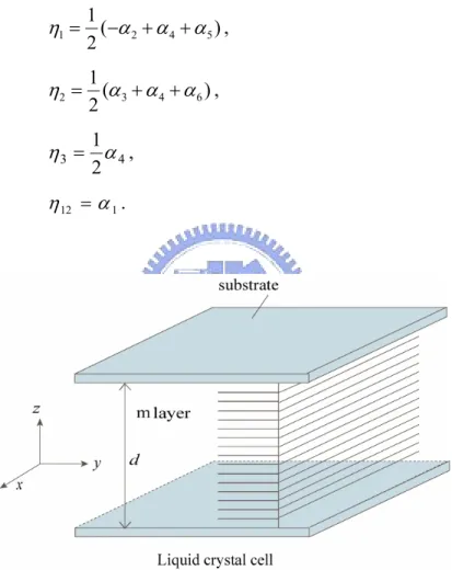
(29) where t ji − π kj n i , k + g j n i = t ij − π ki n j , k + g i n j ,. N i = n& i − wik n k ,. N ij = n& i , j − wik n k , j , 2d ij = v i , j + v j ,i , 2 wij = v i , j − v j ,i , Ni may be interpreted as the angular velocity of the director relative to that of the fluid. It should be emphasized that the stress tensor tji is asymmetric. When ni= 0, (2.14)-(2.17) reduce to the familiar equations of hydrodynamics for an isotropic fluid. The constitutive equation for the qualities gi, tji and πji was developed by Leslie who assumed that these qualities were single-valued function of ni, ni,j , Ni and dij and separated tji and gi into a static (or elastic) part and a hydrodynamic (or viscous) part. t ji = t 0ji + t ' ji ,. gi = gi0 + g 'i. where the superscript 0 denotes the isothermal static deformation value and the prime denotes the hydrodynamic part, g'i is the hydrodynamic part of the director body force, t' ji is the hydrodynamic part of the stress tensor,. t 0ji = − p δ ij −. ∂ f bulk n k ,i ∂ n k ,i. gi0 = γni − β j ni , j −. ∂f bulk ∂ni. π ji = π 0ji + π ' ji = π ji = β j ni +. ∂f bulk ∂ni , j. t ' ji = α 1n k n m d km n i n j + α 2 n j N i + α 3 n i N j + α 4 d ji + α 5 n j n k d ki + α 6 n i n k d kj. (2.18). g 'i = −γ 1 N i − γ 2n j d ji. γ 1 = α 3 − α 2 ( γ 1 : rotational viscosity). (2.19). γ 2 = α6 − α5 where p, γ, and βj are arbitrary constants, π ' ji is the hydrodynamic part which is equal to zero, α1∼ α6 represent the six Leslie coefficients of viscosity of a nematic liquid crystals. 15.

(30) The Paraodi’s relation: α 2 + α 3 = α 6 − α 5. (2.20). In general, the shear viscous coefficients (Miesowicz’s coefficients, η1, η2, η3, η13) and the rotational coefficients can be measured by experiment, the Leslie coefficients then can be derived by shear viscous coefficients. The relationship between the Miesowicz coefficients and the Leslie coefficients of viscosity can be established by substituting the director components and velocity gradients into Eq. (2.18) together with the rotational viscosity (2.19) and the Parodi’s relation (2.20). 1 2. η1 = ( −α 2 + α 4 + α5 ) , 1 2. η2 = (α 3 + α 4 + α 6 ) , 1 2. η3 = α 4 , η 12 = α 1 .. Figure 2.2 The liquid crystal cell, which has infinite extension in the x and y directions, is bounded at z = 0 and z = d. The layer is divided into m equally spaced sub-layers. Fluid velocities and director orientation are functions of z and t only.. The equations for the one-dimension flow problem In our simulation, we suppose that the liquid crystal layer extends to infinity in x-y plane and is bounded at z = 0 and z = d (see Figure 2.2) and the applied electric field is applied along the z-coordinate. Furthermore, we assume all quantities, such as fluid velocities, director orientation, voltage potential and electric field, depend only on the z-coordinate. 16.

(31) We only consider the planar flow of liquid crystals and the z-component of the velocity is assumed to be zero and the boundary directors are rigidly anchored on the substrates and the velocity there is also assumed to be zero. Suppose the LC is an impressible material, in the isothermal process: v v v v n = n ( z, t ), v = v ( z, t ) ni , x = ni , y = vi , x = v i , y = 0 , (i = x, y, z), Therefore, d xz = d zx = wxz = − wzx =. 1 1 v x ,z , d yz = d zy = v y , z , 2 2 1 1 v x , z , w yz = − wzy = v y , z 2 2. d x , y = d y , x = d x , x = d y , y = d z , z = 0 , wx , y = w y , x = wx , x = w y , y = wz , z = 0 1 1 nk nm d km = n y nz v y , z = n x nz v x , z , n z n k d kx = n z2 d z , x = n z2 v x , z , n x n k d kz = (n x n y v y , z + n x2 v x , z ) , 2 2 N x = n& x −. 1 1 1 1 v x , z n z , N y = n& y − v y , z n z , N z = n& z + v x , z n x + v y , z n y , 2 2 2 2. The one-dimensional conservation of linear momentum can be written as: ∂v 1 1 ∂ [( α 2 n z n& x + α 3n x n& z ) + (α 1n y n z2 n x + α 3n y n x + α 6 n x n y ) y ∂z 2 2 ∂z ∂v 1 1 1 1 1 + (α 1n x2 n z2 − α 2 n z2 + α 3n x2 + α 4 + α 5 n z2 + α 6 n x2 ) x ] ∂z 2 2 2 2 2. (2.21). 1 1 ∂ ∂v [( α 2 n z n& y + α 3n y n& z ) + (α 1n y n z2 n x + α 3 n x n y + α 6 n x n y ) x 2 2 ∂z ∂z 1 1 1 1 1 ∂ v + (α 1n 2y n z2 − α 2 n z2 + α 3n 2y + α 4 + α 5 n z2 + α 6 n 2y ) x ] 2 2 2 2 2 ∂z. (2.22). ρ v& x =. ρ v& y =. The equation of motion of the directors:. ρ 1 n&&x = λ n x −. ∂ f bulk ∂ ∂ f bulk ∂v x + − γ 1 n& x − α 2 n z ∂n x ∂z ∂n x ,z ∂z. (2.23). ρ 1n&&y = λ n y −. ∂v y ∂ f bulk ∂ ∂ f bulk + − γ 1n& y − α 2 n z ∂n y ∂z ∂n y ,z ∂z. (2.24). ∂v ∂v ∂ ∂ f bulk ∂ f bulk − γ 1n& z − α 3 n x x − α 3 n y y + ε 0 ∆ ε E z2 n z + ∂z ∂z ∂z ∂n z ,z ∂n z. (2.25). ρ 1n&&z = λ n z −. r where λ is the Lagrange multiplier which is determined by the constrain, n = 1. 17.

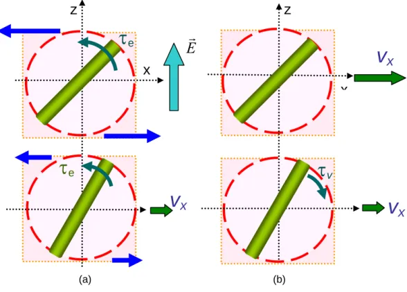
(32) z. z. τe. r E. vx. x x. τe. τv vx. vx. (a) Figure 2.3. (b). The liquid crystal director under an external electric field. The director rotates by the electric. field and induces the movement of the center of mass of the director. The movement of the director will influence the rotation of the director.. In most cases, the liquid crystal system may be regarded as a strongly damping oscillator and the influence of the inertia terms is very small comparison with the viscous terms. We may assume that, after a change of the field strength, a new velocity pattern is established almost instantaneously.. Therefore, the inertia terms can be neglected without losing. significant effects and the left side of Eq. (2.21) to (2.25) equals zero. Figure 2.3 illustrates the flow effects between two layers. Due to the different tilt angles of the directors, the electric torques acting on the directors, which can be derived from Eq. (2.5), are not equal.. Therefore, there are two unequal shear forces acting on the. interface between two layers. Since the liquid crystal is assumed to satisfy the continuum theory and obeys the conservation laws and Oseen’s equation, Eq. (2.21) to (2.25), there is a relative velocity between these two layers, which is illustrated in Figure 2.3 (a). On the other hand, if there is a relative velocity between two layers, an induced torque is produced which is shown in Figure 2.3 (b). These dynamic behaviors are coupled together.. 18.

(33) If we assume there is no flow phenomenon and ignore the inertia term in the motion equation of director, we obtain the general form of the static deformation equation from Eq. (2.23) to (2.25):. ∂ ∂ f bulk ∂f − bulk + λ n i = γ 1 n& i − G i . ∂z ∂ni,z ∂ ni. (2.26). The one dimensional response time (rising time and relaxation time) can be estimated by this equation when the applied forces are not large enough to induce the flow effects.. 2.2 Models of the anchoring energy density The anchoring of liquid crystal (LC) directors at substrates plays a very important role in the performance characteristics of any liquid crystal display (LCD), such as viewing angle, contrast ratio and response time. In the modeling of LCD, the anchoring energy must be included in the calculation. To describe the surface effect, Rapini and Papoular (5) (RP) have introduced a simple phenomenological expression for the interfacial surface anchoring energy per unit area, fs, which describes the interaction between the nematic director and substrate of. 1 homeotropic anchoring: f s = W sin 2 (θ ) , where θ is the polar angle of the director and W 2 is the anchoring energy coefficient, which determines the ability of the director to deviate from the easy axis. Subsequently, many attempts had been carried out to generalize the RP model in order to describe the planar and tilt anchoring(6-9). Becker et al.(6) considered a surface with weak polar and strong azimuthal anchoring. Hirning et al.(7) combined the polar and azimuthal anchoring to an interfacial energy without correlations between them. Sugimura et al.(8-10) used a single coupling constant to describe the interfacial energy. They suggested that the interfacial energy should not be separated into the polar and azimuthal surface anchoring energies, which are independent of each other, as is conveniently carried out. Zhao et. al.(11,12) generalized an RP-type anchoring energy formula with two anchoring coefficients and an orthonormal vector triplet through a second-order spherical harmonic expansion. These models are discussed in the following sections.. 19.

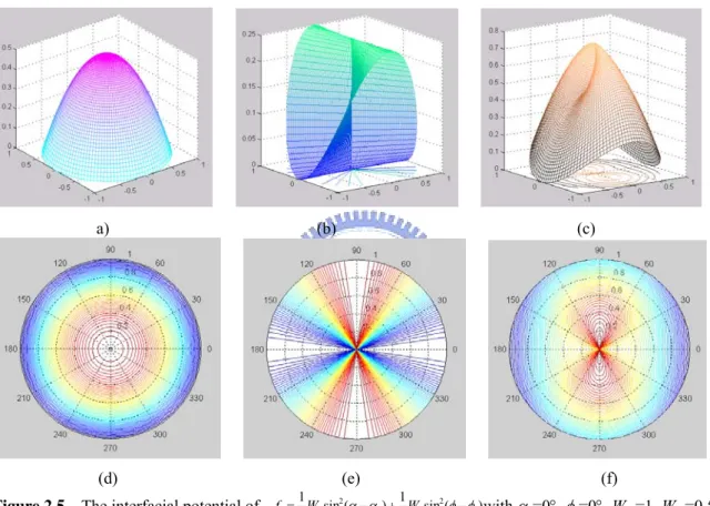
(34) 2.2.1 Rapani-Popular model The interfacial potential of between the surface director and the homeotropic alignment for the Rapani-Papoular model is:. 1 f s = W sin 2 (θ ) , 2. (2.25). where θ is the polar angle of the director and W is the anchoring energy coefficient. Figure 2.4 shows the interfacial potential as a function of the surface director. The surface director is represented by the corresponding points on the x-y plate, which is the projection of the surface directors from z direction. The height in the diagram is the surface anchoring energy density fs.. The interfacial potential is symmetric in the. azimuthal direction and the tilt angle of the easy axis is 90°.. Figure 2.4. The interfacial potential of Rapani-Papoular model. 2.2.2 Other models On the other hand, one of the popular formulas used in the literatures is shown as (7): 1 1 f s = Wθ sin 2 (α − α e ) + Wφ sin 2 (φ − φe ), 2 2. (2.26). where αe and φe are the tilt angle and the azimuthal angle of the easy axis. The fs with. αe=0°, φe=0° and Wθ =1, Wφ =0.5 is plotted in the Figure 2.5. The first and the second column are the polar and azimuthal anchoring energy density of fs, respectively. The third column is the combination of these two energies. The height in the first row and the colors in the second row represent the values of anchoring energy density. We find it oscillates extremely in the azimuthal direction when α near 90° as shown in (b) and (e). This seems 20.

(35) unreasonable and results in a non-smooth shape in the surface anchoring energy density in (c) and (f). Moreover, if the pretilt angle is not zero, the surface free energy should have a minimum at the location of the easy axis. However, from Eq. (2.26), the surface free energy density has two minimum at α = αe and α = 180° − αe. This is irrational since the. r. r. directors which have the property of n = − n , should have the minimum free energy at α = αe and α = 180° + αe. This contradiction can be observed in Figure 2.6 with the pretilt angle of 45°.. a). (b). (d). (c). (e). Figure 2.5 The interfacial potential of. 1 1 f s = Wθ sin2 (α − αe ) + Wφ sin2 (φ − φe ) with 2 2. (f). αe=0°, φe=0°, Wθ =1, Wφ =0.5. (a),. (d) and (b), (e) are the polar and azimuthal anchoring energy portions of fs, respectively. The third column is the combination of these two energies.. The height in the first row and the colors in the second row represent the. values of anchoring energy.. (a). (b) 21. (c).

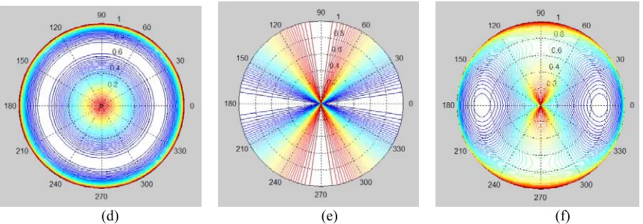
(36) (d) Figure 2.6. (e). (f). 1 1 The interfacial potential of f s = Wθ sin2 (α − αe ) + Wφ sin2 (φ − φe ) with αe=45°, φe=0°, Wθ =1, Wφ =0.5 2 2. The model used by DIMOS The surface anchoring energy density used by commercial simulator DIMOS (autronics-MELCHERS) is: 1 1 f s = Wθ sin 2 (α − α e ) + Wφ sin 2 (φ − φe ) cos 2 α . 2 2. (2.27). With the αe=0°, φe=0° and Wθ =1, Wφ =0.5, we have Figure 2.7. The shapes in (b), (e) and (c), (f) seem more reasonable compared with that of Figure 2.5 in the large α regime. However, the problem of easy axes still exists as shown Figure 2.8 (c) and (f).. (a). (d) Figure 2.7. (b). (c). (e). (f). 1 1 2 2 2 The interfacial potential of f s = 2 Wθ sin (α − αe ) + 2 Wφ sin (φ − φe ) cos α with. = 0.5 22. αe=0°, φe=0°, Wθ =1, Wφ.

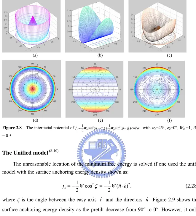
(37) Figure 2.8. (a). (b). (c). (d). (e). (f). The interfacial potential of f s = 1 Wθ sin2 (α − αe ) + 1 Wφ sin2 (φ − φe ) cos2α with 2 2. αe=45°, φe=0°, Wθ =1, Wφ. = 0.5. The Unified model (8-10) The unreasonable location of the minimum free energy is solved if one used the unified model with the surface anchoring energy density shown as: 1 1 f s = − W cos2 ζ = − W ( nˆ ⋅ eˆ) 2 . 2 2. (2.28). where ζ is the angle between the easy axis eˆ and the directors nˆ . Figure 2.9 shows the surface anchoring energy density as the pretilt decrease from 90° to 0°. However, it only uses one anchoring energy coefficient to describe the potential in the azimuthal and polar direction.. The generalized RP model (11,12) Finally, W. Zhao et al. propose a model as a generalized RP model which shown as: 1 1 f s = Wξ ( nˆ ⋅ ξˆ) 2 + Wη ( nˆ ⋅ηˆ ) 2 . 2 2. (2.29). where ( eˆ, ξˆ,ηˆ ) is an orthonormal vector triplet with Euler angles (φe ,θ e ,ψ e ) with respect to ( xˆ , yˆ , zˆ ) and is shown in Figure 2.10. 23.

(38) (a). (b). (c). (d). (f). (g). (h). (i). Figure 2.9 The surface anchoring energy of the unified model as the pretilt decrease from 90° (a) to 45°(c), 25°(f), and 0°(h).. 24.

(39) Figure 2.10 ϕe is the angle between the nodal line and y-axis, θe is the angle between the easy axis and the z-axis, ψe is the angle between the nodal line and η-axis.. Wξ (Wη) is the energy difference between ξˆ (ηˆ ) and eˆ directions. Figure 2.11 shows the surface anchoring energy as the pretilt decrease from 90° to 0°. This model. r. r. successfully solve the problem of n = − n and have two anchoring energy coefficients to describe the movement of the surface directors. For all these models, when the pretilt angle is close to 0° or 90° and the deviation of the surface director is small, the anchoring energy densities are alike. If we only consider the movement of the surface director in the polar direction, one simply adds the pretilt angle αe to the RP model and the anchoring energy density becomes: 1 f s = Wθ sin 2 (α − α e ) . 2. (2.30). This formula implies that the surface director is rigidly anchored in the azimuthal direction and sometimes it is also called PR model.. 25.

(40) (a). (b). (c). (d). (e). (f). (g) (h) Figure 2.11 The surface anchoring energy of the unified model as the pretilt decrease from (a) to 60°(c), 25°(f), and 0°(h).. 26.

(41) References of Chapter 2 1. C. W. Oseen. .The theory of liquid crystals. Trans. Faraday Soc., 29, 883 (1933).. 2. F. C. Frank, .Liquid crystals: On the theory of liquid crystals.. Discuss Faraday Soc., 25, 19 (1958).. 3. J. L. Ericksen, Anisotropic fluids. Arch. Ration. Mech. Anal., 4, 231 (1960).. 4. F. M. Leslie, Some constitutive equations for liquid crystals, Arch. Ration. Mech. Anal., 28, 265 (1968).. 5. A. Rapini, and M. Papoular, J. Phys. (Paris) Colloq., 30, C4-54, (1969).. 6. M. E. Becker, J. Nehring, and T. J. Scheffer, J. Appl. Phys., 57, 4539, (1985).. 7. R. Hirning, W. Funk, H. R. Trebin, M. Schmidt, and H. Schmiedel, J. Appl. Phys., 70, 4211, (1991).. 8. A. Sugimura, O. Y. Zhong-can, Phys. Rev. E., 51, 784, (1995).. 9. A. Sugimura, G. R. Luckhurst, O. Y. Zhong-can, Phys. Rev. E., 52, 681, (1995).. 10. A.Sugimura, T. Miyamoto, M.Tsuji and M. Kuze, Appl. Phys. Lett. 72, 329 (1998).. 11. W. Zhao, C. X. Wu, and M. Iwamoto, Phys. Rev. E., 62, R1481, (2000).. 12. Wei Zhao, Chen-Xu Wu and Mitsumasa Iwamoto, Phys. Rev. E, 65, 031709, (2002).. 27.

(42) Chapter 3. Study on the anchoring energy density In order to understand the influence of the anchoring properties on the dynamic behaviors, we have to know the coordinates of the easy axis first. The coordinate of the easy axis means the azimuthal and the tilt angle of the easy axis. The tilt angle of the easy axis is so called the pretilt angle. Since the electric fields are usually applied in the surface normal direction, the study is focused on the behaviors of the LC directors in the polar direction. To measure the pretilt angle, several techniques of LC cells have been proposed in the literature (1−5), such as the magnetic null method (1), the crystal rotation technique(2,3), the polarizer rotation method(4) and the phase retardation measurement method (5). These methods are accurate and reliable for the pretilt angle measurement of the transmissive cells. However, one has to modify these methods in order to measure the reflective cells, which either complicates the set-up (1−4) or limits itself to the large pre-polar angle measurement. (5). .. In the former part of this chapter, we propose a method to. determine the pretilt angle of the VA reflective LC cells; moreover, this method can also be applied to the transmissive cells. Once the easy axis is confirmed, we are ready to measure the anchoring properties of the LC cells. The anchoring energy density model usually used for measuring the polar anchoring energy coefficient is PR model with the formula of Eq. (2.30). The commonly used method to determine the polar anchoring energy density coefficient is the high-electric-field (HEF) method (6,7), in which the coefficient of the polar anchoring energy (Wθ,RP) is determined within the high applied electric field regime.. However, the negative. Wθ,RP values are sometimes obtained (8). In fact, the director distortions calculated from the RP formula do not agree well with the observations in strong external fields. Since a large applied field causes large deviation angles, the adaptability of the RP model is 28.

(43) questioned and the anchoring energy density requires modification.. In later part of this. chapter, we adopt a modified polar anchoring energy density to determine the coefficients of some non-twisted cells.. 3.1 Determination of the pretilt angle of the reflective liquid crystal cells Reflective liquid crystal display (R-LCD) has been widely used because of their low power consumption, lightweight, and outdoor readability. The characteristics of R-LCD, such as brightness, contrast ratio, and response time, are determined by the cell gap, twist angle, pretilt angle etc., and the measurements of these parameters are still developing (9-12). Among the modes used in LCD, vertically aligned (VA) mode exhibits excellent dark state, which is a nice candidate to be used in the R-LCD e.g. LCoS (Liquid Crystal on Silicon). The pre-polar angle (measured from the substrate normal) of VA-LCD is usually less than 5° and is crucial for the dark state.. Therefore, an accurate measurement method to. determine the pre-polar angle of a VA-R-LCD is desired. In this section, we propose a field induced birefringence method to determine the pre-polar angle of the VA-R-LCD with low pre-polar angle. We derive theoretically the field induced optical phase retardation, which is linearly proportional to the square of the applied voltage and the pre-polar angle in the small molecular deformation regime for the small pre-polar angle. This linear relation exists not only for the reflective but also for the transmissive VA-LCD. Based on the theoretical analysis, we can determine the pretilt angle of the VA-R-LCD by measuring the phase retardation with a simple optical system. In the experiments, three liquid crystal cells were prepared. We measured the phase retardation as a function of applied voltage in two VA reflective cells and obtained the pre-polar angles from the slopes of the fitting lines in the low voltage regime.. We also determined the. pre-polar angle of one transmissive VA cell by this method and the result agrees well with the pre-polar angle obtained by crystal rotation technique.. 3.1.1 Theory As we know that when there is no pretilt angle on both substrates of a vertically aligned liquid crystal cell with hard boundary assumption, the tilt angles of the directors remain 29.

(44) zero up to the Fredericks transition threshold voltage. If the cell has nonzero pretilt angle, there is no threshold, and the phase retardation will increase as the applied voltage increases. To obtain the relation between the phase retardation and the applied voltage, we begin with Frank’s elastic free energy density under the continuum theory to calculate the director profile of LC cell under an applied voltage. We define the polar angle θ(z) as the angle from the normal direction of the cell to the LC director. The free energy per unit surface area is expressed as: F =. 2 ⎫⎪ 1 d ⎧⎪ D z2 ⎛ dθ ⎞ 2 2 θ θ ( k sin k cos ) + + ⎟ ⎜ ⎨ ⎬ dz , 11 33 2 2 ∫ 2 0 ⎪⎩ ⎝ dz ⎠ ε 0 (ε // cos θ + ε ⊥ sin θ ) ⎪⎭. (3-1). where Dz represents the electrical displacement in z direction, which is uniform throughout the cell, k11 and k33 are the Frank elastic constants for splay and bend deformations respectively, ε // and ε ⊥ stand for the longitudinal and transverse dielectric constants of the liquid crystals and d is the cell gap. We assume that the directors on the boundaries are fixed with the polar angle θ0 and we call it pre-polar angle. That is, the pretilt angle is (90° − θ0). The relation between θ(z) and the applied voltage V can be obtained by minimizing the free energy density in eq. (3-1), which is: θm V 2 (1 + κ sin 2 θ ) dθ , = (1 + γ sin 2 θ m ) ∫ θ0 Vth π (1 + γ sin 2 θ )(sin 2 θ m − sin 2 θ ). where θm is the polar angle of the mid-layer directors, Vth = π. (3-2). k −k k33 , κ = 11 33 ε 0 (ε ⊥ − ε // ) k33. ε ⊥ − ε // . ε // Once we have θ(z), we can calculate the phase retardation Γ(V) from the following. and γ =. equation:. Γ (V ) =. 4π. λ. ∫. d 0. ⎡ ⎢ ⎣. ne no n e2. 2. cos θ. ( z ) + n o2. 2. sin θ ( z ). ⎤ − n o ⎥ dz , ⎦. (3-3). where ne and no stand for the extraordinary and ordinary refractive indices of LC material respectively, and λ is the wavelength of incident light. In order to obtain an analytic solution, we focus our attention at low applied voltage and small deformation regime. The polar angle of the mid-layer directors can be express as 30.

(45) θm=θ 0 +∆θm, where θ 0 >0, and ∆θm ≥0. By series expansion with respect to ∆θm, we have the relation between the applied voltage V and ∆θm : 1/ 2. V ⎛ ∆θ m ⎞ ⎟ =⎜ Vth ⎜⎝ θ 0 ⎟⎠. When. θ 02 <<. ⎡ 2 2 (2 + 3κ ) 2 2 ⎤ ⎛ ∆θ ⎞ + θ 0 + ....⎥ + ⎜⎜ m ⎟⎟ ⎢ 3π ⎣ π ⎦ ⎝ θ0 ⎠. 6 (2 + 3κ ). ⎡⎛ ∆θ ⎞3 / 2 ⎛ 5 ⎞⎤ ⎢⎜⎜ m ⎟⎟ ⎜ ⎟⎥ ⎢⎣⎝ θ0 ⎠ ⎝ 3π 2 ⎠⎥⎦. ∆θ m θ0. and. <<. 3/ 2. 2.4,. 5 ⎡ ⎤ ⎢− 3π 2 + ....⎥ + .... . ⎣ ⎦. (3-4). which. from. is. deduced. ⎡⎛ ∆θ ⎞1/ 2 ⎛ 2 2 ⎞⎤ ⎟⎥ << 1, Eq. (3-4) is approximately reduced to ⎢⎜⎜ m ⎟⎟ ⎜⎜ ⎟ ⎢⎣⎝ θ0 ⎠ ⎝ π ⎠⎥⎦. ∆ θ m (V ) = θ m (V ) − θ 0 ≈. π 2V 2 8V th2. θ0 .. (3-5). Substitute Eq. (3-5) into ∆ θ m θ 0 << 2.4, and we have the limitation of the voltage: 2. π 2V 2 8V th2 << 2.4. It means that when V << 1.95 V th2 , ∆θm is linearly proportional to V. 2. approximately. Similarly, we derived the relation between the phase retardation and ∆θm as: Γ (V ) = Γ ( 0 ) +. 4πn o d ⎧⎛ ∆ θ m ⎨⎜ λ ⎩⎜⎝ θ 0. ⎛ ∆θ + ⎜⎜ m ⎝ θ0. where ν = (ne2 − no2 ) ne2 .. ⎞ ⎡ 2ν 2 ⎤ 4⎞ ⎟⎟ ⎢ θ 0 + ν ⎛⎜ν − ⎟θ 04 + .... ⎥ 9⎠ ⎝ ⎦ ⎠⎣ 3. 2 ⎫⎪ ⎞ ⎡11ν 2 ⎤ ⎟⎟ ⎢ θ 0 + ... ⎥ + ... ⎬, ⎦ ⎪⎭ ⎠ ⎣ 45. When θ 02 << 6 (9ν − 4 ). ⎡ ⎛ ∆ θ ⎞ 2 ⎛ 11ν 2 ⎞ ⎤ deduced from ⎢ ⎜⎜ m ⎟⎟ ⎜ θ 0 ⎟⎥ ⎠ ⎥⎦ ⎢⎣ ⎝ θ 0 ⎠ ⎝ 45. (3-6). and ∆ θ m θ 0 << 2.73, which is. ⎡ ⎛ ∆ θ m ⎞ ⎛ 2ν 2 ⎞ ⎤ ⎟⎟ ⎜ θ 0 ⎟ ⎥ , Eq. (3-6) is reduced to: ⎢ ⎜⎜ ⎠⎦ ⎣⎝ θ 0 ⎠⎝ 3. Γ (V ) − Γ ( 0 ) ≈. 8π n o d ν ∆ θ m . θ0 3λ. (3-7). By substituting eq. (3-5) into eq. (3-7), we have. ∆Γ (V ) = Γ (V ) − Γ ( 0 ) ≈. π 3 ( ne2 − no2 ) no d θ 02 2 V . 3n e2 λ Vth2. (3-8). We analyze the limitations of the applied voltage from the range of the deformation: one is 31.