Robust stability analysis of a fuzzy vehicle lateral control system using describing function method

P. Melin et al. (Eds.): Anal. and Des. of Intel. Sys. using SC Tech., ASC 41, pp. 769–779, 2007. springerlink.com © Springer-Verlag Berlin Heidelberg 2007

Lateral Control System Using Describing

Function Method

Jau-Woei Perng1_{, Bing-Fei Wu}1_{, Tien-Yu Liao}1_{, and Tsu-Tian Lee}2 1 _{Department of Electrical and Control Engineering, National Chiao Tung}

University 1001, Ta-Hsueh Road, 300 Hsinchu, Taiwan

[email protected], [email protected], [email protected]

2 _{Department of Electrical Engineering, National Taipei}

University of Technology 1, Sec. 3, Chung-Hsiao E. Rd. 106 Taipei, Taiwan [email protected]

Abstract. In this paper, the robust stability analysis of a fuzzy vehicle lateral system with

per-turbed parameters is presented. Firstly, the fuzzy controller can be linearized by utilizing the describing function method with experiments. After the describing function is obtained, the sta-bility analysis of the vehicle lateral control system with the variations of velocity and friction is then carried out by the use of parameter plane method. Afterward some limit cycle loci caused by the fuzzy controller can be easily pointed out in the parameter plane. Computer simulation shows the efficiency of this approach.

Keywords: Describing function, vehicle lateral system, fuzzy control, parameter plane,

limit cycle.

1 Introduction

It is well known that the describing function is an useful frequency domain method for analyzing the stability of a nonlinear control system especially when the system has hard nonlinear elements, such as relay, deadzone, saturation, backlash, hystere-sis and so on. The fundamental description of describing functions can be referred in [1-3]. Some academic and industry researches have been applied the describing function to meet the design specifications. For PI controller design, an iterative pro-cedure for achieving gain and phase margin specifications has been presented in [4] based on two relay tests and describing function analysis. In [5], the describing function utilized for the stability analysis and limit cycle prediction of nonlinear control systems has been developed. The hysteresis describing function was applied to the class AD audio amplifier for modeling the inverter [6]. Ackermann and Bunte [7] employed the describing function to predict the limit cycles in the parameter plane of velocity and road tire friction coefficient. The algorithm computes the limit cycles for a wide class of uncertain nonlinear systems was considered in [8]. As for the intelligent control, some researchers have developed the experimental and

analytic describing functions of fuzzy controller in order to analyze the stability of fuzzy control systems [9-11]. Besides, the describing function was also applied to find the bounds for the neural network parameters to have a stable system response and generate limit cycles [12]. In fact, the uncertainties are often existed in the practical control systems. It is well known that the frequency domain algorithms of parameter plane and parameter space [13, 14] have been applied to fulfill the robust stability of an interval polynomial.

In this paper, we apply the describing function of fuzzy controller mentioned in [11] and parameter plane method [14] to consider the robust stability of a vehicle lateral control system with perturbed parameters. A systematic procedure is proposed to solve this problem. The characteristics of limit cycles can be found out in the pa-rameter plane. Computer simulation results verify the design procedure and show the efficiency of this approach.

2 Description of Vehicle Model and Design Approach

In this section, the classical linearized single track vehicle model is given first. The describing function of fuzzy controller is also introduced. In order to analyze the sta-bility of perturbed parameters, a systematic procedure is proposed to solve this prob-lem by the use of parameter plane method. In addition, the control factors are also addressed.

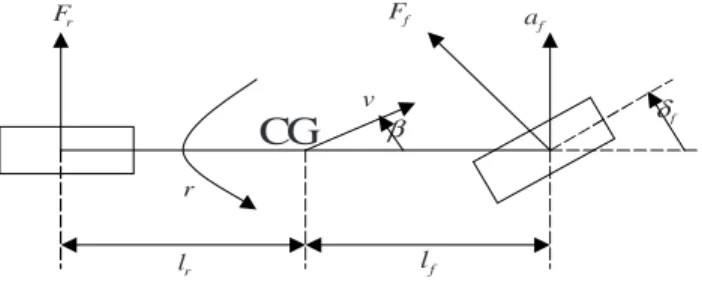
2.1 Vehicle Model [7]

Figure 1 shows the single track vehicle model and the related symbols are listed in Table 1. The equations of motion are

( ) f r f f r r f r F F mv r F l F l ml l r β ⎡ + ⎤ ⎡ + ⎤ = ⎢ ⎥ ⎢ ₋ ⎥ ⎢ ⎥ ⎣ ⎦ ⎣ ⎦ & & (1) The tire force can be expressed as

0 0

( ) , ( )

f f f f r r r r

F α =μ αc F α =μ αc (2) with the tire cornering stiffnesses cf0,cr0, the road adhesion factor μ and the tire side slip angles

( f ), ( r ) f f r l l r r v v α =δ − β+ α = − −β (3)

The state equation of vehicle dynamics with

β

0 0 0 0 0 2 2 2 0 0 0 0 0 ( ) ( ) 1 ( ) ( ) f r r r f f f f f r r f f f f r r r f r f r c c c l c l c mv mv mv c c l c l c l c l r r ml ml l ml l v μ μ _μ β β _δ μ μ μ + − ⎡ ⎤ ⎡ ⎤ − − + ⎢ ⎥ ⎢ ⎥ ⎡ ⎤ _{⎢ ⎥}⎡ ⎤ _{⎢ ⎥} = + ⎢ ⎥ _{⎢ − + ⎥}⎢ ⎥ _{⎢ ⎥} ⎣ ⎦ ⎣ ⎦ _{⎢ − ⎥ ⎢ ⎥} ⎢ ⎥ ⎣ ⎦ ⎣ ⎦ & & (4)

r F Ff r

CG

Fig. 1. Single track vehicle model

Table 1.Vehicle system quantities

front wheel steering angle

mass wheelbase

distance from fro nt and rear axis to C G lateral acceleratio n

velocity

side slip angle at center of gravity (CG) yaw rate

lateral wheel force at front and rear wheel

front wheel steering angle

mass wheelbase

distance from fro nt and rear axis to C G lateral acceleratio n

velocity

side slip angle at center of gravity (CG) yaw rate

lateral wheel force at front and rear wheel , f r F F r β v f a , f r l l f r l=l +l f δ m

Table 2. Vehicle parameters

1.32 m 1.51 m 1830 kg 100000 N/rad 50000 N/rad 1.32 m 1.51 m 1830 kg 100000 N/rad 50000 N/rad 0 f c 0 r c m f l r l

Hence, the transfer function from δf to r is 2 2 0 0 0 2 2 2 2 2 2 0 0 0 0 0 0 ( ) ( ) f f f f r r f r r r f f f r r r f f c ml v s c c l v G l l m v s l c l c l m vs c c l c l c l m v δ μ μ μ μ μ + = + + + + − (5)

The numerical data in this paper are listed in Table 2.

According to the above analysis of a single track vehicle model, the transfer func-tion from the input of front deflecfunc-tion angle δf to the output of yaw rate r can be

obtained as 8 2 10 2 6 2 2 9 7 2 10 2 (1.382 10 1.415 10 ) ( , , ) 6.675 10 1.08 10 (1.034 10 4 10 ) f r v s v G s v v s vs v δ μ = _{× +} ×_× μ_μ +₊ ×_× μ_{μ + × μ} (6)

The operating area Q of the uncertain parameters μ and v is depicted in Fig. 7. In addition, the steering actuator is modeled as

2 2 2 ( ) 2 n A n n G s s s ω ω ω = + + (7) where ωn=4π .

The open loop transfer function G sO( ) is defined as ( , , ) ( ) ( , , )

f

O A r

G s

μ

μ

2.2 Describing Function of Fuzzy Controller

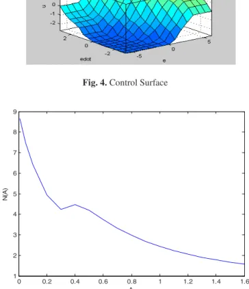
In this subsection, the fuzzy controller given in [11] is adopted here. Figure 2 shows the block diagram for determining the describing function of the fuzzy controller from experimental evaluations. The membership functions of the fuzzy controller are shown in Fig. 3 (a)-(c) and the rules of the fuzzy controller are listed in Table 3. Figure 4 shows the control surface. According to the analysis in [11], the describing function ( )N A with input signal ( ( )x t =Asinωt) and scaling factors (k_p =6,

0.001

d

k = ) can be obtained in Fig. 5.

x p k d k dt d e e d o t u Fuzzy Controller

(a) Input of e

(b) Input of edot

(c) Output of u

Fig. 3. Fuzzy membership functions

Table 3. Rules of the fuzzy controller

PV PV PV PV PS PM ZE PV PV PV PV PS PM ZE NM PS PV PV PS PM ZE NM NS PM PV PS PM ZE NM NS NV ZE PS PM ZE NM NS NV NV NM PM ZE NM NS NV NV NV NS ZE NM NS NV NV NV NV NV PV PS PM ZE NM NS NV PV PV PV PV PS PM ZE PV PV PV PV PS PM ZE NM PS PV PV PS PM ZE NM NS PM PV PS PM ZE NM NS NV ZE PS PM ZE NM NS NV NV NM PM ZE NM NS NV NV NV NS ZE NM NS NV NV NV NV NV PV PS PM ZE NM NS NV e edot

Fig. 4. Control Surface 0 0.2 0.4 0.6 0.8 1 1.2 1.4 1.6 1 2 3 4 5 6 7 8 9 A N( A )

Fig. 5. Describing function of the fuzzy controller

Vehicle Dynamics R r r x + -u s k p k d k dt d Fuzzy Controller ( , , ) o G sμv c δ e edot u

2.3 Parameter Plane Method

Figure 6 shows the overall block diagram of a fuzzy vehicle lateral control system. In this study, ku =0.1 is selected. After some simple manipulations by using (5) to (8), the characteristic equation in Fig. 6 can be obtained as

2 2 2 2 4 3 2 1 0 ( , , ) 0 f s v C C v C v C v C v μ μ μ μ μ = + + + + = , (9) where 10 2 4 4.0045 10 ( 17.7715 157.9137) C = × s s + s+ , 6 3 2 3 6.675 10 ( 17.7715 157.9137) C = × s s + s+ , 9 2 2 2 1.0746 10 ( 17.7715 157.9137) C = × s s + s+ , 11 1 2.2345 10 1 C = × N , 8 2 9 0 1.03395 10 ( 17.7715 157.9137) 2.1818 10 1 C = × s s + s+ + × N s.

Let s= j

ω

( , , ) 0 f jω μ v = +X jY= (10) where 11 2 2 12 4 2 9 4 11 2 11 2 9 2 2 1 1 7.1165 10 1.0075 10 (1.0746 10 1.6970 10 ) 2.2345 10 1.8375 10 , X v v N v N v ω μ ω ω ω μ μ ω μ = − × + × + × − × + × − × 12 10 3 2 6 5 9 3 2 10 3 10 8 3 9 2 1 (6.3236 10 4.0045 10 ) (6.6750 10 1.0541 10 ) 1.9098 10 (1.6327 10 1.03395 10 2.1818 10 ) . Y v v N v ω ω μ ω ω ω μ ω ω ω μ = × − × + × − × − × + × − × + ×

In order to obtain the solution of μ and v , the following equation is solved 0 0 X Y = ⎧ ⎨ ₌ ⎩ , (11) when kp, kd, ku, N1 are fixed and ω is changed from 0 to ∞. As the amplitude A is changed, the solutions of μ and v called limit cycle loci can be displayed in the parameter plane.

3 Simulation Results

In this work, the scaling factors of k_p =6, 0.001kd = , and ku =0.1 in Fig. 6 are

above section. So the describing function of the fuzzy controller shown in Fig. 5 can be applied to analyze the stability of the closed loop system. After doing so, the solu-tion of (11) can be solved when A is fixed and ω is changed from 0 to ∞. Figure 7 shows the operating area of the vehicle system. Two limit cycle loci in the μ-v pa-rameter plane as A=0.1 and A=0.2 are plotted in Fig. 7, respectively. In order to test the predicted result in Fig. 7, eight operating points with Q1 (

μ

μ

μ

μ

μ

30

v= ), Q6(

μ

μ

μ

0 10 20 30 40 50 60 70 80 0 0.2 0.4 0.6 0.8 1 1.2 1.4 1.6 v (m/sec) mu Q A=0.2 A=0.1 Q1(67,1) Q2(56,1) Q3(65.8,0.75) Q4(54.2.0.63) Q5(30,1) Q6(30,0.37) Q7(5,1) Q8(5,0.1)

Fig. 7. Operating area and limit cycle loci

0 10 20 30 -0.5 0 0.5 1 Q1 x( t) 0 10 20 30 -0.5 0 0.5 1 Q2 0 10 20 30 -0.5 0 0.5 1 Q3 Time (sec) x( t) 0 10 20 30 -0.5 0 0.5 1 Q4 Time (sec)

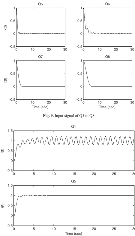
0 10 20 30 -0.5 0 0.5 1 Q5 x( t) 0 10 20 30 -0.5 0 0.5 1 Q6 0 10 20 30 -0.5 0 0.5 1 x( t) Q7 Time (sec) 0 10 20 30 -0.5 0 0.5 1 Q8 Time (sec)

Fig. 9. Input signal of Q5 to Q8

0 5 10 15 20 25 30 -0.5 0 0.5 1 1.5 r( t) Q1 0 5 10 15 20 25 30 -0.5 0 0.5 1 1.5 Q5 r( t) Time (sec)

the time simulations. Figure 8 shows the time responses of the input signal ( )x t at Q1 to Q4. The limit cycles are existed when operating at these four points and it consists with the predicted results (the amplitude of limit cycles) in Fig. 7.

On the other hands, the time responses of the input signal ( )x t at the other four points are displayed in Fig. 9. No limit cycle occurs in these four cases and this result is also matched with Fig. 7. Finally, the unit step responses of the output signal ( )r t at two operating points Q1 and Q5 are given in Fig. 10.

4 Conclusions

Based on the approaches of describing function and parameter plane, the robust stabil-ity of a fuzzy vehicle lateral system is considered in this paper. A systematic proce-dure is presented to deal with this problem. Simulation results show that more information about the characteristic of limit cycle can be obtained by this approach.

Acknowledgments. This paper is supported by the National Science Council in Taiwan through Grant NSC95-2752-E009-010.

References

1. Gelb A, Velde W. E. V.: Multiple Input Describing Functions and Nonlinear System De-sign. McGraw-Hill, New York (1968)

2. Siljak, D. D.: Nonlinear Systems - The Parameter Analysis and Design. New York: Wiley (1969).

3. Atherton, D. P.: Nonlinear Control Engineering. Van Nostrand Reinhold Company, Lon-don (1975)

4. Arruda, G. H. M., Barros, P. R.: Relay-Based Gain and Phase Margins PI Controller De-sign. IEEE Trans. Instru, and Measure. Vol 52 5 (2003) 1548-1553

5. Krenz, G. S., Miller, R. K.: Qualitative Analysis of Oscillations in Nonlinear Control Sys-tems: A Describing Function Approach. IEEE Trans. Circuits and Systems. Vol. CAS-33 5 (1986) 562-566

6. Ginart, A. E., Bass, R. M., Leach, W. M. J., Habetler, T. G.: Analysis of the Class AD Au-dio Amplifier Including Hysteresis Effects. IEEE Trans. Power Electronics. Vol. 18 2 (2003) 679-685

7. Ackermann, J., Bunte, T.: Actuator Rate Limits in Robust Car Steering Control. Prof. IEEE Conf. Decision. and Control. (1997) 4726-4731

8. Nataraj, P. S. V., Barve, J. J.: Limit Cycle Computation for Describing Function Approxi-mable Nonlinear Systems with Box-Constrained Parametric Uncertainties. Int. J. of Robust and Nonlinear Cont. Vol. 15 (2005) 437-457

9. Gordillo, F., Aracil, J., Alamo, T.: Determining Limit Cycles in Fuzzy Control Systems. Proc. IEEE Int. Conf. Fuzzy Syst. Vol. 1 (1997) 193-198

10. Kim, E., Lee, H., Park, M.: Limit-Cycle Prediction of a Fuzzy Control System Based on Describing Function Method. IEEE Trans. Fuzzy Syst. Vol. 8 1 (2000) 11-21

11. Sijak, T., Kuljaca, O., Tesnjak, S.: Stability Analysis of Fuzzy Control System Using De-scribing Function Method. MED2001. Dubrovnik, Croatia (2001)

12. Delgado, A.: Stability Analysis of Neurocontrol Systems Using a Describing Function. Proc. Int. Join. Conf. Neural Network. Vol. 3 (1998) 2126-2130

13. Siljak, D. D.: Parameter Space Methods for Robust Control Design: A Guide Tour. IEEE Trans. Automat. Contr. Vol. 34 7 (1989) 674-688

14. Han, K. W.: Nonlinear Control Systems - Some Practical Methods. Academic Cultural Company, California (1977)