因應退休準備之投資策略的探討(III)

行政院國家科學委員會專題研究計畫 成果報告

因應退休準備之投資策略的探討(第 3 年)

研究成果報告(完整版)

計 畫 類 別 ： 個別型 計 畫 編 號 ： NSC 97-2410-H-004-165-MY3 執 行 期 間 ： 99 年 08 月 01 日至 100 年 07 月 31 日 執 行 單 位 ： 國立政治大學風險管理與保險學系 計 畫 主 持 人 ： 黃泓智 計畫參與人員： 碩士班研究生-兼任助理人員：林思岑 處 理 方 式 ： 本計畫涉及專利或其他智慧財產權，2 年後可公開查詢

中 華 民 國 100 年 10 月 30 日

Optimal Asset Allocation of Defined Contribution Pension Plans

1. Introduction

Defined contribution (DC) pension plans have become quite popular in the global pension market. With a DC scheme, employers transfer the pension fund investment risk to employees, and most DC plans cannot provide sufficient pension benefits with a conservative investment strategy. However, an aggressive strategy may possibly suffer the high risk that the pensioner will end up with a small accumulated pension fund. Therefore, employees must choose their strategies carefully during the accumulation phase to attain better benefits without suffering too much investment risk.

Mortality improvements complicate this issue. Many countries face serious aging problems as their populations age significantly and simultaneously feature low fertility rates. The resulting longer expected retirement phase makes it crucial to include improved mortality into retirement planning. Longevity risk also has a vital impact on economic security during a postretirement phase, because insufficient pensions will be a serious issue.

Accordingly, we investigate two main issues in this paper. First, we attempt to find an appropriate method to predict future mortality. Second, we pursue a suitable strategy to prepare and accumulate required wealth by incorporating longevity risk during a person’s working lifetime. To capture longevity risk predictions more precisely, we apply a time adjustment of the mortality trend to the mortality model.

The significant increases in population life expectancy have prompted a variety of mortality models in the past two decades [e.g., Lee and Carter 1992; CMI 1999; Lin and Cox, 2005; Cairns et al., 2006, 2007, 2008]. Among them, the Lee-Carter model has gained a wide acceptance and proved to be an effective method for estimating mortality. Although some other models offer better mortality estimation performance [e.g., Cairns et al., 2007, 2008], they also suffer the disadvantage of more parameters. However, problems still plague the Lee-Carter model. For example, it assumes a certain pattern of change in the age distribution of mortality [Lee, 2000], even though mortality data often show that the relative speed of decline at different ages may vary. The Lee-Carter model cannot take such pattern shifts into account, so some researchers select a shorter database, but it has proved difficult to assess which periods of mortality trends are more suitable as a basis for projections [Wilmoth, 2005; Janssen and Kunst, 2007]. Previous mortality literature tends to focus on improving mortality estimations rather than improving mortality predictions. We focus on future mortality predictions and adapt the Lee-Carter model by applying the concept of time

adjustment to reflect the mortality trend over time, such that recent mortality rate data takes greater weight in the estimation. Our approach reflects prior evidence that shows forecast performance improves when the forecast integrates the time adjustment factor.

We also investigate the optimal multiperiod asset allocation during the accumulation phase for a DC plan in a discrete time model. Extensive research into the optimal investment strategy largely concentrates on continuous time and solves the closed form solution with dynamic control [e.g., Devolder et al., 2003; Battocchio and Menoncin, 2004; Gerrard et al, 2004; Hainaut and Devolder, 2007; Romaniuk, 2007] or the martingale method [e.g., Boulier et al., 2001; Deelstra et al, 2003]. However, most of these two approaches are applied in continuous time. Even though the discrete investment decision progression describes real-world behavior well, it remains relatively rare in the literature. Haberman and Vigna [2001, 2002] apply dynamic programming in discrete time and derive a closed form solution by establishing a time-independent asset return process. But their approach depends on a well-devised problem and a well-designed model, such that any violation of the assumptions results in mathematical complexity and intractability.

Thus, to examine the appropriate investment strategy in discrete time, we must trade off between the rationality of the method and the accuracy of the solution. Blake et al. [2001] examine a range of asset allocation strategies, including both static and simple dynamic forms, for a range of asset return models. They specify investment strategies at the inception of a DC pension plan and observe the performance distribution at retirement. Following Blake et al. [2001], Blake et al. [2007] examine the impact of occupation and gender in the likely retirement income available from DC pension plans. Yang and Huang [2009] examine the interaction between longevity risk and asset allocation for a defined contribution pension plan; their result shows a life cycle investment strategy and indicates that longevity risk can be hedged by either raising the contribution rate or setting a more aggressive strategy. Huang and Lee [2010] deal with the asset allocation issue for a general portfolio of life insurance policies. They consider the static optimal investment strategies for a time-dependent asset return process in discrete time.

This paper presents a discrete-time pension fund management model for a DC plan by investigating the static, multiperiod optimal investment strategy. The asset return model is consistent with Huang and Lee [2010] so that theoretical formulae for the first two moments for the accumulated pension fund can be replicated straightforwardly. We then adopt optimization programming to find a multi-period asset allocation that fits the DC pension plan.

basis. In this paper, we first argue that the predictability of the most popular cohort mortality model, the Lee-Carter model, might be improved by integrating of time adjustment. The word “time adjustment” refers to the greater weight on the recent mortality rate data in the estimation on the parameters of the Lee-Carter model. We then present a discrete-time pension fund management model for a DC plan to examine optimal investment strategies for three different mortality prediction cases: a naïve choice, which predicts mortality according to a period life table; a general choice, or predicting mortality with the Lee-Carter model; and the technique proposed by our study, which predicts mortality according to the time adjustment.

Our investigations offer three main findings. First, according to the U.S. male mortality data, the enhancement of the logarithm death rate for ages 50–85 years, which affects the value of the annuity primary, has been increasing in the last two observed periods (i.e., from 1981 to 2004). This shift becomes clear from the Lee-Carter model if we consider a time-weighted adjustment. Second, optimal investment strategies should be more aggressive if the contribution rate does not increase. Third, we confirm the validity of the so-called lifestyle investment strategy, as widely adopted by investment managers in DC pension plans (see Yang and Huang [2009]).

The structure of this paper is as follows: We discuss the mortality issue in the next section. In Section 3, we present the DC pension scheme as well as the asset return process. We then investigate the optimal asset allocation for the DC plan and illustrate a numerical example in Section 4. Finally, Section 5 contains our conclusions.

2. The moments of the accumulated pension fund

Most literature regarding pension funds appears in the context of aggregate investment return rates, such as independent and identically distributed (i.i.d.) returns or AR or MA time-series models (Haberman, 1994, 1997; Cairns and Parker, 1997; Bedard, 1999; Haberman, Butt and Megaloudi, 2000; Bedard and Dufresne, 2001; Perry, Stadje and Yosef, 2003). In contrast, we employ a multi-asset model (Huang and Cairns 2006) to consider the asset allocation issue regarding a DC pension scheme. The moments of the accumulated pension fund are functions of the investment decisions (i.e., asset allocations), and we can control for asset allocation to achieve a pension target (e.g., 70% retirement replacement ratio).

2.1. Accumulated pension fund formula

At the inception of the accumulation period for a DC pension plan, the future accumulation value after n years, F(n), can be expressed as

 

1

   

0 n j F n CF j I j   



(1) where CF(j) is the yearly contribution amount at the start of year j+1, and I(j) is the accumulation factor from time j to the retirement date n. We assume that the fund value is 0 before the first contribution, CF(0).

By ignoring mortality processes in the accumulation phase and assuming that the contribution amounts are measurable at time 0, the first two moments of accumulation value F(n) is:

 

1

 

 

0 n j E F n CF j E I j         



  (2) and

 

1 1

   

   

0 0 , n n j k Var F n CF j CF k Cov I j I k           



  (3)

2.2. Asset return model and the moments of the accumulated pension fund

Huang and Cairns (2006) propose a discrete asset return model that includes three assets: a one-year bond (cash), a long-dated bond, and an equity asset. The logarithm return rate between time t1 and t for each of these assets is denoted by y t(  , 1)

 

b t

 , and _e

 

t , respectively, with the following underlying processes1:

 





 





 

 

 





 





 

 

 

( 1) ( ( 2) ) ( 1) 1 1 1 1 y y b b b by y b b e e e ey y eb b e e y t y y t y Z t t y t t y t Z t Z t t y t t y t Z t Z t Z t                   _{         }   _{          }  (4)

where Z_y

 

t , Z_b

 

t , and Z t_e

 

are N

 

0,1 random variables, independent of one another and i.i.d. through time t. The time indicator of the parentheses represents

the measurability of the random variables. For example, Z t_y(  and ( 1)1) y t are

measurable at time t1, whereas Z_y

 

t , Z_b

 

t and _b

 

t are not measurable until time t.

Suppose p proportion of the fund is invested in equities and _1t p proportion is _2t invested in long-dated bonds at time t1, with the remaining account invested in cash. Using a second-order Taylor approximation2 of the nonlinear function that relates the logarithm of individual-asset returns to logarithm portfolio returns, we can

1

Please see chapter 2.1 of Campbell and Viceira (2002) for a general form of this asset model.

2

For more discussion about this approximation, please refer to chapter 2.1 of Campbell and Viceira (2001).

write the logarithm return on the fund from t1 to t , Z t

 

, as

 



 







 

_{ }













 

_{ }

 





1 1 2 1 2 1 2 2 1 2 1 2 ln 1 1 1 ( 1) , , , 2 2 1 ( 1) , , 0 e ee t t t t t t t b bb t e ey eb e y t t t t b by b b e Z t i t t v p y t p p p p p p t v p Z t y t p p p p Z t Z t                  _                  _{ }    _{  }   _{ }    

(5)

where













 

 



 

 



1 1 2 1 2 1 2 2 1 1 , , , , 2 2 , , , and , ee t t t t t t t bb t ee eb ee e bb b eb e b eb bb v p p p p p p p v p v v

v Var t v Var t v Cov t t

v v   _ _ _ _            _{ }      .

Huang and Lee [2010] examine the asset allocation issue for a general portfolio of life insurance policies under this asset return model. They derive the explicit formulae for the first two moments of accumulated asset value. By replicating their model, we can obtain the moments of the accumulation pension fund. We then set asset allocations appropriately to control pension funds to get a predetermined target. The explicit formulae for the expectation of I(j) in equation (6) and the covariance between I(j) and I(k) in equation (7) are list in Appendix A.

3. Optimal multiperiod asset allocations for DC pension plans

We assume that an employee starts his career at age x and plans to retire at age x+n. During his working life, a fixed percentage of his salary gets contributed annually, in advance, to his personal pension fund. Let W(t) be the annual salary at age x+t and F(t) denote the level of the pension fund at time t, according to the accumulated process described by equation (5). If we assume the salary of the employee grows yearly with a fixed force  3 and ignore mortality during the accumulation phase, the level of the employee’s pension fund at retirement depends only on investment performance.

3.1. The pension fund target

For an individual retiree, the retirement replacement ratio is the most popular

3

indicator to assess the suitability of retirement income. We assume an employee will accumulate his pension fund to match a target retirement replacement ratio (RR). Moreover, to keep the annuity increasing with inflation, we assume that this life annuity will grow with a fixed force of inflation rate  annually.

Define a_{x n ,} as the present value of an annuity of 1, payable immediately, that grows with the force of inflation  annually to a retiree at age x+n, calculated as

    , 0 x n j x n j x n j a e p           



  (6) where  is a constant force of interest, _jp_{x n} is the probability that a person of age x+n will survive at least j years, and  is the maximum survival age. Thus, the goal of the employee is to choose a suitable portfolio strategy that will keep the fund value

at retirement near W n



 1



RR a _{x n ,}.

The annuity factor a_{x n ,} cannot be measured until the employee’s retirement date. In addition to mortality risk, the employee faces an interest rate risk at retirement. We focus the effect on mortality perception and simply assume the annuity discounting factor,  , equals the long-term average level of cash, y . Accordingly, the unique factor relates to the value of a_{x n ,} , and the target pension liability



1



x n,

W n RR a _{ } is mainly the mortality process.

We assume that an employee chooses the following quadratic objective function to achieve a prespecified retirement replacement ratio4:

 





1 2 2 , min , 0,1,..., -1 t t p p E F n Q t n  _  _   , (7) where Q is the target pension liability, and QW n



 1



RR a _{x n ,}. To calculate

,

x n

a _{ }

 , we need the mortality prediction for age x+n. A naïve choice uses the mortality rate of the last period life table, ignoring the sustained improvement of the historical data. Another option relies on a well-developed mortality model to predict future

4

Quadratic objective function has been widely used in the literature regarding investment strategies for DC plans, e.g., see Vigna and Haberman [2001], Haberman and Vigna [2002], Gerrard et al, [2004] and Yang and Huang [2009].

mortality, such as the Lee-Carter model. We offer a third choice, namely, a mortality prediction that considers time adjustments to avoid underestimating target pension liability. We also provide a numerical example to demonstrate the difference among these three choices of mortality predictions.

3.2 Numerical results

In this section, we provide a numerical application to illustrate the optimal asset allocations among the three mortality prediction choices. We assume that a 30-year-old employee will retire 30 years later. His contribution rate to the pension fund is 8% of his salary annually, with an annual salary growth rate 3%. We set the initial salary of the employee to 1 without losing generality. His target pension liability is to reach 70% of the retirement replacement ratio, and we calculate the target pension liability Q according to the three mortality predictions (see Table 1). The first case (Case 1) directly adopts the period life data for 2004. The second case (Case 2) predicts mortality according to the Lee-Carter model with the SVD approach. Finally, the third case (Case 3) predicts mortality using the Lee-Carter model with the time adjustment factor, for which we assume the employee applies joint weighted with h0.8 to predict the future mortality.

We use Matlab 7.0.4 to find the minimum value of the objective function (equation (11)). Function “fminunc” is used when there is no short constraint and “fmincon” is employed when there is short constraint. Parameters of asset return model are consistent with that of Hunag and Lee [2010]5.

3.2.1 Target pension liability among three choices

According to Table 1, the target pension liability for Case 1 is the smallest, because we do not consider any mortality improvement. In addition, the target pension liability in Case 2 is smaller than that for Case 3, because we do not take the time adjustment into account in the Lee-Carter model, which means we underestimate the mortality improvement for ages beyond 57 years. Therefore, we underestimate the target pension liability.

Table 1. Mortality prediction methods and the corresponding values of target pension liability

Mortality prediction method  =2%  =6%

Case 1 period life table, 2004 21.4495 32.4414

5  _0.828 , y0.0666,  _b 0.0102,  _e 0.0215, _y 0.0141, _b 0.0798, 0.0260 by    , _e 0.1957, _ey  0.0128, _eb0.0432, and y

 

0 0.0666.

Case 2 SVD approach 23.3093 37.0823

Case 3 joint weighted, h=0.8 23.9614 38.8090

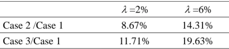
Table 2 shows the percentage we underestimate the target liability for different pensions increases ( ) when we ignore mortality improvement or time adjustment. As Table 4 reveals, if the pension increasing rate  is 2%, we underestimate the value of Q by 8.67% when we ignore the mortality improvement. If we do not consider time adjustment, we further underestimate Q by another 3%. In addition, if

 is 6%, the magnitude of the underestimation grows even worse. For example, the percentage of underestimation increases from 8.67% to 14.31% when we fail to consider mortality improvements, and the percentage of underestimation increases from 11.71% to 19.63% when we ignore time adjustments. In other words, if the design of annuity products focuses more on inflation protection, the percentage of underestimation becomes more serious as a result of the failure to consider mortality improvements or time adjustments.

Table 2. Underestimation of the target pension liability Q compared with period life table

 =2%  =6%

Case 2 /Case 1 8.67% 14.31%

Case 3/Case 1 11.71% 19.63%

3.2.2 Numerical results of optimal asset allocations

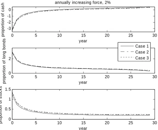
In this subsection, we investigate the optimal asset allocation of cash, long-term bonds, and equities for a target liability in the DC pension plan. Figure 1 depicts the optimal asset allocation for an annual liability of a 2% ( =2%) pension increase, without the short constraint. Thus, the employee should invest more in long-term bonds (300%) and equities (130%) and short lots of cash (300%) at the beginning of the term. The optimal investments then shift gradually from long-term bonds and equities into cash, which seems intuitively reasonable, because employees should be more risky early in the term to accumulate the fund faster and then gradually switch to riskless assets to match their target liability. Similar results exist for  = 6% (see Figure B1 in Appendix B). The optimal asset allocation looks quite similar for Cases 1, 2 and 3 in Figure 1 and Figure C1. Figure C2 (Appendix B) shows the differences in the holdings for each asset between Case 1 and Case 2 and between Case 2 and Case 3 when  = 6%; it indicates that the employee should increase the proportion of long-term bonds to near 6% and increase equities 4.7% from Case 1 to Case 2, and then increase the proportion of long-term bonds to near 2% and increase equities 1.5%

from Case 2 to Case 3. The employee also should short an extra 10.7% of cash from Case 1 to Case 2 and an extra 3.5% of cash from Case 2 to Case 3.

0 5 10 15 20 25 30 -3 -2 -1 0 pr op or ti on o f c a s h year

annually increasing force, 2%

0 5 10 15 20 25 30 0 2 pr op or ti on o f long b o n d s year 0 5 10 15 20 25 30 0 0.5 1 1.5 pr opo rt ion of s to c k s year Case 1 Case 2 Case 3

Figure 1. Optimal asset allocations of Cases 1, 2, and 3 when  =2% and there is no short constraint.

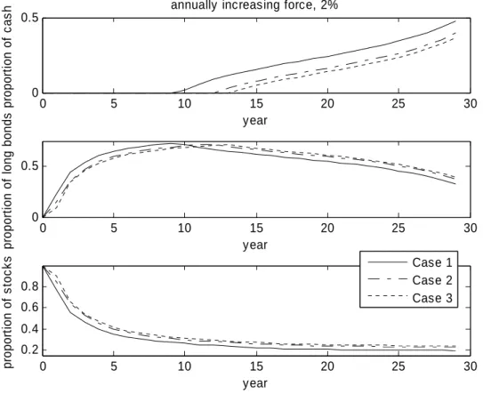
The optimal asset allocation in Figure 5 is not realistic, because it is not possible to short so much cash to buy long-term bonds and equities in practice. Therefore, for greater realism, we add a short constraint to the optimization process and show, in Figure 2, the optimal asset allocation in this case. In Case 1, the employee should hold a very high proportion of equities in the early years of the term (100% in the first year) and then gradually reduce the proportion of equities in later years (20% in the last year). The employee should not invest any cash in the first nine years and then gradually increase the proportion of cash from the tenth year until maturity (50% in the last year). Unlike from the results in Figure 1, Figure 2 suggests the employee should not hold any long-term bonds in the first year because he or she cannot short cash to buy long-term bonds. The proportion of long-term bonds should gradually increase from the second to the tenth year to increase investment returns, and then gradually decline to the last year (30%) to reduce the investment risk and match the target pension liability. In addition, we show the optimal asset allocation with a

consideration of mortality improvements (Case 2) and time adjustments (Case 3) in Figure 2. The employee should invest more aggressively in Case 3, which makes sense, because for the larger target pension liability of Case 3, the employee should hold more risky assets to earn more profits and match the larger liability. Thus, the employee should start to hold cash after the thirteenth year in Case 2 and the fourteenth year in Case 3, as well as increase the proportion of equities nearly 4% from Case 1 to Case 2 and nearly 1.4% from Case 2 to Case 3.

0 5 10 15 20 25 30 0 0.5 pr op or ti on o f c a s h year

annually increasing force, 2%

0 5 10 15 20 25 30 0 0.5 pr op or ti on o f long b o n d s year 0 5 10 15 20 25 30 0.2 0.4 0.6 0.8 pr opo rt ion of s to c k s year Case 1 Case 2 Case 3

Figure 2. Optimal asset allocations for Cases 1, 2, and 3 when  = 2% and there are short constraints.

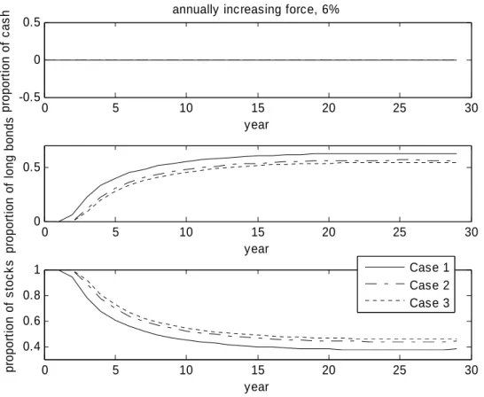
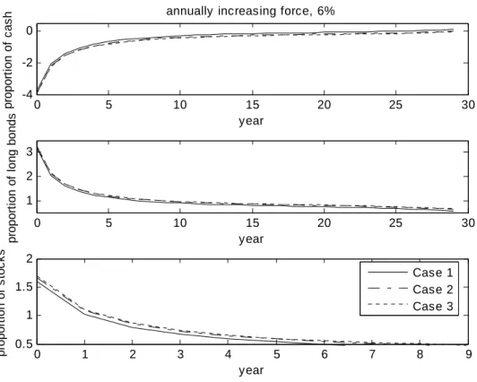
If we change the annual rate at which the pension increases from 2% to 6%, the target pension liability increases from 51% to 62%6 for Cases 1, 2, and 3 (see Table 1). Therefore, if the employee does not increase his or her contribution rate, he or she should switch to more aggressive investment strategies. Figure 3 further suggests that in Cases 1, 2, and 3, the employee does not hold any cash during the term but instead retains high proportions of assets in equities, and then gradually switches to long-term bonds to match target liabilities. For example, in Case 1, the employee should hold all assets in equities in the first two years and gradually reduce the equity proportion to near 40% in the last year. For Case 3, he or she should hold all assets in equities

6

during the first three years and then gradually reduce the equity proportion to nearly 50% in the last year. Compared with Cases 1 and 2, the most aggressive investment strategy occurs in Case 3. In other words, on average, people should invest 6.6% more in equities, according to the model with mortality improvements, and an additional 2.1% more in equities, according to the time adjustment model.

0 5 10 15 20 25 30 -0.5 0 0.5 pr op or ti on o f c a s h year

annually increasing force, 6%

0 5 10 15 20 25 30 0 0.5 pr op or ti on o f long b o n d s year 0 5 10 15 20 25 30 0.4 0.6 0.8 1 pr opo rt ion of s to c k s year Case 1 Case 2 Case 3

Figure 3. Optimal asset allocations of Cases 1, 2, and 3 when  = 6% and there are short constraints.

4. Conclusion

In DC pension plans, employees are responsible for their pension funds, but in general, the amount they accumulate is not sufficient. Investment returns become key means to increase pension funds, which makes it essential for employees to choose the optimal investment strategies during accumulation phases to ensure a stronger accumulated pension fund after their retirement but without suffering too much investment risk. Moreover, mortality improvement significantly affects the need for pension preparation. Longer retirement phases demand the inclusion of mortality improvements in retirement planning, because improved mortality requires more accumulated wealth. Therefore, we first investigate an appropriate method to predict future mortality properly, then examine the optimal asset allocation for a DC pension

plan, both with and without longevity risk. In addition, to capture longevity risk predictions more precisely, we apply time adjustments to the mortality model.

Our numerical results show that if we fail to consider any mortality improvement, we underestimate the target pension liability by approximately 8.67% to 14.31% when the annual pension increases from 2% to 6%. If we ignore both mortality improvement and time adjustment, we might underestimate the target pension liability by 11.71% to 19.63% for the same annual pension increases. Regarding the optimal asset allocation of the DC pension plan, the numerical results suggest investing more funds in long-term bonds and equities at the beginning of the term and then gradually shifting to cash, an intuitively reasonable recommendation, because investors should hold more risky assets early in the term to accumulate the fund faster and then switch to riskless assets to match target liability. This result also confirms the validity of the so-called lifestyle investment strategy, which is widely adopted by investment managers in DC pension plans.

In addition, investors should be more aggressive, according to the results that include mortality improvements or time adjustments. For larger target pension liabilities, investors should hold more risky assets to earn more profits and match the greater liabilities, which is consistent with Yang and Huang [2009]. However, the greater the proportion on holding risky assets corresponds to the greater volatility of the final fund level, and thus the greater volatility of the replacement ratio. To deal with this issue, some alternative solutions may be considered, e.g., raising contribution rate, cutting down target and/or deferring retirement. This is outside of the scope of this study, which leaves for the topic for future research.

Appendix A

Moments of the accumulation factor, I(j). (Please see Huang and Lee [2010] for a detailed proof.)

Define p as the proportion of the fund invested in equities and _1t p as the _2t proportion of the fund invested in long-dated bonds at time t1. Then,

(a) Define Z t

 

as the logarithm return of the fund from t1 to t . The expected value, variance, and covariance of Z t

 

at the valuation date, t0, are

 



 



1









1 2 1 2 0 t _t, _t e _t, _t b E Z t_   _ y y y    p p _ _ p p    ,

 

2



2( 1)







1 1 2 2 2 1 , 1 y t t t t t p Var Z t p p p            _{ }   _  , and

  



2 2( 1) 1





1 2 2 , (1 ) , ; 1 ey y t k k t t y by Cov Z t Z t k     p p   k N            _{ }     _   . (b) Define

 

 

1 k j S k Z j 





. The accumulation factor I k

 

, depending on the actuarial portfolio selection of the employee, will be

 

exp



   



I k  S n S k . Moreover, the expected value, variances, and covariance of S k

 

at the valuation date are:

 







1 2





1 2



1 1 (0) , , 1 k k e j j j j j b E S k ky y y  p p  p p              _{  } _   _{  }  



,

 





 





















 









2 ₂ 1 1 2 2 2 2 1 1 1 1 2 2 1 2 2 1 2 1 , 1 1 1 1 2 1 1 1 1 1 1 1 1 2 , 1 k k j y j j j j k _k k k y k j ey j j by p Var S k k p p p k p p  _         _            _            _  _ _{ }   _{ }       _               _ _     _  _{ }



1 1 k y j    



, and

  



 

_



_

_



_



_



_





_

_

2 1 2 1 2 1 1 1 1 , 1 1 1 1 , 1 m k k y k j m k ey j j y by j Cov S k S k m Var S k p p                              _{  }  _{  }     _{ }   _{ }   



.

(c) At the valuation date, the moments of the accumulation factor, I j

 

, expressed by the moments of S j

 

, are

 

 

 

1



 





 





   



exp 2 ,

2

E I j_ _ _E S n_ _E S j_ _ _Var S n Var S j  Cov S n S j _

 

   

exp



j k, j k,



E I j I k_ _ C D

   

,

   

 

 

Cov I j_ I k _E I j I k_ _E I j_  _{ }E I k _{ ,} where C_{j k,} 2E S n_

 

_



E S j_

 

_E S k_

 

_{ ,}



and

























, 4 ( ) 4 ( ), ( ) 4 ( ), ( ) 1 2 ( ) 2 ( ), ( ) ( ) j k

Var S n Cov S n S j Cov S n S k

D

Var S j Cov S j S k Var S k

              . Appendix B

0 5 10 15 20 25 30 -4 -2 0 pr op or ti o n o f c a s h year

annually increasing force, 6%

0 5 10 15 20 25 30 1 2 3 p rop or ti o n of l o ng bo nd s year 0 1 2 3 4 5 6 7 8 9 0.5 1 1.5 2 p rop or ti o n of s toc k s year Case 1 Case 2 Case 3

Figure B1. Optimal asset allocations of Case 1, 2 and 3 when  =6% and there is no short constraint. 0 5 10 15 20 25 30 -0.1 -0.05 0 di ff e re n c e of c a s h year

annually increasing force, 6%

0 5 10 15 20 25 30 0 0.05 0.1 di ff e re nc e of l o ng b o n d s year 0 5 10 15 20 25 30 0 0.05 0.1 0.15 di ff e re nc e of s toc k s year Case 2-Case 1 Case 3-Case 2

Figure B2. The difference of asset holding for each asset between Case 1 and Case 2 and between Case 2 and Case 3 when  =6% and there is no short constraint.

References

Battocchio, P., Menoncin, F., 2004. Optimal pension management in a stochastic framework. Insurance: Mathematics and Economics 34, 79-95.

Be´dard, D., 1999. Stochastic pension funding: proportional control and bilinear processes. ASTIN Bulletin 29, 271-293.

Be´dard, D., Dufresne, D., 2001. Pension funding with moving average rates of return. Scandinavian Actuarial Journal 2001, 1-17.

Blake, D., Cairns, A. J. G., Dowd, K., 2001. Pensionmetrics: stochastic pension plan design and value-at-risk during the accumulation phase. Insurance: Mathematics and Economics 29, 187-215.

Blake, D., Cairns, A. J. G., Dowd, K., 2007. The impact of occupation and gender on pensions from defined contribution plans. Geneva Papers on Risk and Insurance - Issues and Practice 32, 458-482.

Boulier, J.F., Huang, S., Taillard, G., 2001. Optimal management under stochastic interest rates: The case of a protected defined contribution pension fund. Insurance: Mathematics and Economics 28, 173–189.

Cairns, A. J. G., Blake, D., Dowd, K., 2006. A two-factor model for stochastic mortality with parameter uncertainty: Theory and calibration. Journal of Risk and Insurance 73, 687-718.

Cairns, A.J.G., Blake, D., Dowd, K., 2008. Modelling and management of mortality risk: a review. To appear in Scandinavian Actuarial Journal.

Cairns, A.J.G., Blake, D., Dowd, K., Coughlan, G.D., Epstein, D., Ong, A., Balevich, I., 2007. A quantitative comparison of stochastic mortality models using data from England and Wales and the United States. Working paper.

Cairns, A.J.G., Parker, G., 1997. Stochastic pension fund modeling. Insurance: Mathematics and Economics 21, 43-79.

Campbell, J.Y., Viceira, L.M., 2002. Strategic Asset Allocation: Portfolio Choice for Long-term Investors. Oxford: Oxford University Press.

CMI Committee, 1999. Standard tables of mortality based on the 1991-1994 experiences. Continuous Mortality Reports 17, Institute and Faculty of Actuaries, 1-227.

Deelstra, G., Grasselli, M., Koehl, P.F., 2003. Optimal investment strategies in the presence of a minimum guarantee. Insurance: Mathematics and Economics 33, 189–207.

Devolder, P., Bosch, P.M., Dominguez, F.I., 2003. Stochastic optimal control of annuity contracts. Insurance: Mathematics and Economics 33, 227-238.

Gerrard, R., Haberman, S., Vigna, E., 2004. Optimal Investment Choices Post-Retirement in a Defined Contribution Pension Scheme. Insurance:

Mathematics and Economics 35, 321-342.

Haberman, S., 1994. Autoregressive rates of return and the variability of pension contributions and fund levels for a defined benefit pension scheme. Insurance: Mathematics and Economics 14, 219-240.

Haberman, S., 1997. Stochastic investment return and contribution rate in a defined benefit pension scheme. Insurance: Mathematics and Economics 19, 127-139. Haberman, S., Butt, Z., Megaloudi, C., 2000. Contribution and solvency risk in a

defined benefit pension scheme. Insurance: Mathematics and Economics 27, 237-259.

Haberman, S., Vigna, E., 2002. Optimal investment strategy and risk measures in defined contribution pension schemes. Insurance: Mathematics and Economics 31, 35-69.

Hainaut, D., Devolder, P., 2007, Management of a pension fund under mortality and financial risks. Insurance: Mathematics and Economics 41, 134-155.

Huang, H. C., Cairns, A. J. G., 2006. On the control of defined-benefit pension plans. Insurance: Mathematics and Economics 38, 113-131.

Huang, H.C., Lee, Y.T., 2010, Optimal asset allocation for a general portfolio of life insurance policies, Insurance: Mathematics and Economics, 46, 2, 271-280. Janssen, F., Kunst, A., 2007. The choice among past trends as a basis for the

prediction of future trends in old-age mortality. Population Studies 61, 315-326. Lee, R., 2000. The Lee-Carter method for forecasting mortality, with various

extensions and applications. North American Actuarial Journal 4, 80-93.

Lee, R. D., Carter, L. R., 1992. Modeling and forecasting U.S. mortality. Journal of the American Statistical Association 87, 659-675.

Lin, Y., Cox, S. H., 2005. Securitization of mortality risks in life annuities. Journal of Risk and Insurance 72, 227-252.

Perry, D., Stadje, W., Yosef, R., 2003. Annuities with controlled random interest rates. Insurance: Mathematics and Economics 32, 245-253.

Renshaw, A. E., Haberman, S., 2006. A cohort-based extension to the Lee-Carter model for mortality reduction factors. Insurance: Mathematics and Economics 38, 556-570.

Romaniuk, K., 2007. The optimal asset allocation of the main types of pension funds: a unified framework. Geneva Risk and Insurance Review 32, 113-128.

Vigna, E., Haberman, S., 2001. Optimal investment strategy for defined contribution pension schemes. Insurance: Mathematics and Economics 28, 233-262.

Wilmoth, J. R., 1993. Computational methods for fitting and extrapolating the Lee-Carter model of mortality change. Technical report, Berkeley, University of California.

Wilmoth, J. R., 2005. Overview and discussion of the social security mortality projections. Working paper, department of demography, Berkeley, university of California.

Yang, S.S., Huang, H.C., 2009. The impact of longevity risk on the optimal contribution rate and asset allocation for defined contribution pension plans. Geneva Papers on Risk and Insurance: Issues and Practice 34, 4, 660-681.

國科會補助計畫衍生研發成果推廣資料表

日期:2011/10/30

國科會補助計畫

計畫名稱: 因應退休準備之投資策略的探討 計畫主持人: 黃泓智 計畫編號: 97-2410-H-004-165-MY3 學門領域: 財務

無研發成果推廣資料

97 年度專題研究計畫研究成果彙整表

計畫主持人：黃泓智 計畫編號：97-2410-H-004-165-MY3 計畫名稱：因應退休準備之投資策略的探討 量化 成果項目 實際已達成 數（被接受 或已發表） 預期總達成 數(含實際已 達成數) 本計畫實 際貢獻百 分比 單位 備 註 （ 質 化 說 明：如 數 個 計 畫 共 同 成 果、成 果 列 為 該 期 刊 之 封 面 故 事 ... 等） 期刊論文 0 0 100% 研究報告/技術報告 0 0 100% 研討會論文 0 0 100% 篇 論文著作 專書 0 0 100% 申請中件數 0 0 100% 專利 已獲得件數 0 0 100% 件 件數 0 0 100% 件 技術移轉 權利金 0 0 100% 千元 碩士生 0 0 100% 博士生 0 0 100% 博士後研究員 0 0 100% 國內 參與計畫人力 （本國籍） 專任助理 0 0 100% 人次 期刊論文 0 0 100% 研究報告/技術報告 0 0 100% 研討會論文 0 0 100% 篇 論文著作 專書 0 0 100% 章/本 申請中件數 0 0 100% 專利 已獲得件數 0 0 100% 件 件數 0 0 100% 件 技術移轉 權利金 0 0 100% 千元 碩士生 0 0 100% 博士生 0 0 100% 博士後研究員 0 0 100% 國外 參與計畫人力 （外國籍） 專任助理 0 0 100% 人次

其他成果

(

無法以量化表達之成 果如辦理學術活動、獲 得獎項、重要國際合 作、研究成果國際影響 力及其他協助產業技 術發展之具體效益事 項等，請以文字敘述填 列。) 無 成果項目 量化 名稱或內容性質簡述 測驗工具(含質性與量性) 0 課程/模組 0 電腦及網路系統或工具 0 教材 0 舉辦之活動/競賽 0 研討會/工作坊 0 電子報、網站 0 科 教 處 計 畫 加 填 項 目 計畫成果推廣之參與（閱聽）人數 0

國科會補助專題研究計畫成果報告自評表

請就研究內容與原計畫相符程度、達成預期目標情況、研究成果之學術或應用價

值（簡要敘述成果所代表之意義、價值、影響或進一步發展之可能性）

、是否適

合在學術期刊發表或申請專利、主要發現或其他有關價值等，作一綜合評估。

1. 請就研究內容與原計畫相符程度、達成預期目標情況作一綜合評估

■達成目標

□未達成目標（請說明，以 100 字為限）

□實驗失敗

□因故實驗中斷

□其他原因

說明：

2. 研究成果在學術期刊發表或申請專利等情形：

論文：□已發表 □未發表之文稿 ■撰寫中 □無

專利：□已獲得 □申請中 ■無

技轉：□已技轉 □洽談中 ■無

其他：（以 100 字為限）

目前正在撰寫中, 預計在一個月內會投搞到 Journal of Risk and Insurance

3. 請依學術成就、技術創新、社會影響等方面，評估研究成果之學術或應用價

值（簡要敘述成果所代表之意義、價值、影響或進一步發展之可能性）（以

500 字為限）

本研究有推導出有關退休金資產配置的封閉解, 具有學術價值, 應該有機會被國際一流 期刊 Journal of Risk and Insurance 接受.