Effects of multivalent salt addition on effective charge of dilute colloidal
solutions
Tzu-Yu Wang
Department of Chemical and Materials Engineering, National Central University, Jhongli 320, Taiwan, Republic of China
Yu-Jane Shenga兲
Department of Chemical Engineering, National Taiwan University, Taipei 106, Taiwan, Republic of China Heng-Kwong Tsaob兲
Department of Chemical and Materials Engineering, National Central University, Jhongli 320, Taiwan, Republic of China
共Received 21 August 2006; accepted 17 October 2006; published online 21 November 2006兲 The effective charge Z* is often invoked to account for the accumulation of counterions near the
colloid with intrinsic charge Z. Although the ion concentrations ciare not uniform in the solution due to the presence of the charged particle, their chemical potentials are uniform everywhere. Thus, on the basis of ion chemical potential, effective ion concentrations ci*, which can be experimentally measured by potentiometry, are defined with the pure salt solution as the reference state. The effective charge associated with the charged particle can then be determined by the global electroneutrality condition. Monte Carlo simulations are performed in a spherical Wigner-Seitz cell to obtain the effective charge of the colloid. In terms of the charge ratio␣= Z*/ Z, the effects of added salt concentration, counterion valency, and particle charge are examined. The effective charge declines with increasing salt concentration and the multivalent salt is much more efficient in reducing the effective charge of the colloidal solution. Moreover, the extent of effective charge reduction is decreased with increasing intrinsic charge for a given concentration of added salt. Those results are qualitatively consistent with experimental observations by electrophoresis. © 2006 American Institute of Physics.关DOI:10.1063/1.2390707兴
I. INTRODUCTION
A colloidal dispersion, consisting of many charged par-ticles and small ions, is a very complicated system. To de-scribe the equilibrium and dynamic properties of colloidal solutions, the concept of effective charge is commonly adopted in the literature.1–4 The essential idea associated with charge renormalization is that counterions accumulate in the vicinity of the surface of the colloid carrying intrinsic charge Z because of strong electrostatic coupling. That is, the electrostatic attraction is large compared to the thermal en-ergy kBT. Consequently, the decorated object 共charged par-ticle plus counterions兲 may be regarded as a single entity which possesses an effective charge, Z*. The effective charge 共in absolute value兲 can be much less than the intrinsic charge, Z*ⰆZ. The determination of Z* is dependent on
which physical property is considered. It is frequently re-garded as an adjustable parameter in a fit of experimental data with approximated models. For instance, the effective charge can be inferred from voltammetry, electrophoresis, or small-angle neutron scattering.5–8
The concept of effective charge basically characterizes a battle fought between energy and entropy in minimizing the free energy of a solution of mobile charges in the
neighbor-hood of charged particles. For a charged sphere of size a, the electric potential energy of a counterion on the surface is finite,s⬃−Z/a. The entropy associated with the counterion is proportional to kBT ln V with the available volume V. At infinite dilution 共V→⬁兲, the isolated, charged sphere is un-able to bind a counterion at finite temperature and the effec-tive charge is the intrinsic charge, Z*= Z. However, in all
practical colloidal systems, the counterion entropy is finite, ⬃kBT ln c, owing to finite counterion concentration c. As a result, it is expected that charge renormalization takes place eventually when the electrostatic energy gain overcomes the counterion entropy loss.
Theoretically, the effective charge can be determined ac-cording to various definitions. The simple and intuitive defi-nition is the two-state scenario, i.e., condensed and free counterions. The boundary between the two states is arbi-trarily defined. For example, one can choose the position r* at which the local concentration of counterions c共r*兲 equals
the mean value 具c典, i.e., c共r*兲=具c典. Since the counterions
between the particle surface and the chosen boundary neu-tralize an equivalent number of charges on the particle, the effective charge is thus the rest charge of the charge carried by the particle.5Similarly, one can also define the boundary as the location where the interaction energy of the counterion with the parent particle is equal to the thermal energy.9 Nonetheless, such definitions of effective charge do not re-late to thermodynamic quantities of colloidal solutions. a兲Electronic mail: [email protected]
b兲Electronic mail: [email protected]
Another approach in determining the effective charge is the electric field felt by a counterion far from the parent particle.1The electric potential profile is often calculated by the Poisson-Boltzmann 共PB兲 mean-field theory. Because of the mathematical difficulty caused by its nonlinear nature, a linearized approximation is typically employed to obtain analytical expressions. This well-known Debye-Hückel共DH兲 approximation is justified as the thermal fluctuation domi-nates over the electrostatic interaction. Therefore it is inad-equate in describing highly charged particles because the electrostatic energy of counterions near the particle’s surface exceeds the thermal energy. Far from the charged surface, however, the electrostatic potential still follows the DH ex-pression since the thermal energy becomes dominant. By matching the analytical DH solution with Z* to the “exact” numerical solution with Z at a distance away from the par-ticle, the effective charge is obtained. Similarly, the long dis-tance behavior of the exact electrostatic repulsion between two identical colloids with Z can be matched by the effective pair potential with Z* based on the DH approximation. The
latter accounts for screening of the intrinsic charge by coun-terions. Since the effective pair potential is closely related to physical properties such as the bulk modulus of the colloidal crystals,1the effective charge based on this definition may be extracted from experiments.
The DH approach can be generalized to all physical properties associated with a salt-free dispersion. For a ther-modynamic propertysuch as osmotic pressure, its relation to the intrinsic charge Z*may be available under the
condi-tion of weak coupling, i.e.,DH共Z*兲. If we obtain the
prop-ertyof a colloidal solution with intrinsic charge Z, then the effective charge of this dispersion is defined as Z* if DH共Z*兲=共Z兲. The advantage of the DH approach is that
analytical expressions are generally available for various properties and further uses. Nonetheless, this method may be inadequate to display the microscopic picture near the charged particle, particularly for the existence of multivalent counterions. Monte Carlo simulations3,10have shown that for a salt-free dispersion with multivalent counterions, some physical properties, such as chemical potential and surface potential, do not reach a plateau value for large intrinsic charges, but instead they pass through a maximum, and de-crease again as Z inde-creases. This consequence indicates that for two salt-free colloidal dispersions containing charged particles of the same size and volume fraction, their thermo-dynamic property, in particular, , may be the same even though they possess different particle charges Z*and Z, i.e.,
共Z*兲=共Z兲. As a result, one may define Z*as the effective
charge for the dispersion with Z if Z⬎Z*. There exists a
maximally attainable value ofat which Z = Z*.
In a salty dispersion, the effective charge associated with a colloid may be altered due to the screening effect. The charge renormalization based on the far-field behavior re-veals that for low intrinsic charge, Z* is only slightly
changed as a substantial amount of monovalent electrolyte is added.1For ionic strength up to five times that of counteri-ons, Z* changes by approximately 10%. In general, on the basis of the DH approach, the effective charge is increased with the added salt concentration for a fixed Z. On the other
hand, as the intuitive two-state model is used, the effective charge declines with increasing salt concentration.11 Since the added salt itself can have direct contributions to some thermodynamic properties, the definitions of Z* based on
such thermodynamic properties are unable to provide insight on the effect of salt addition on the effective charge. Besides the existing contradiction and difficulty, the added salt in most studies is monovalent. The addition of multivalent salt, however, can lead to significant ion-ion correlation and strong coupling between colloid and multivalent counterion. In this paper, we explore the effects of multivalent salt addition on the effective charge of a dilute colloidal disper-sion on the basis of ion chemical potential. In Sec. II we propose an effective charge, which is thermodynamically well defined and can be determined by potentiometry experi-ments. This definition is essentially equivalent to the ionic activity coefficient in a pure salt solution. In Sec. III the details of Monte Carlo simulations in a spherical Wigner-Seitz cell are briefly described. The residual chemical poten-tials of ions共activity coefficients兲 are calculated and thereby the effective concentrations of coions and counterions can be obtained. In Sec. IV the effective charge of a colloid is de-termined based on the global charge neutrality condition. First, we examine the effective charge of a salt-free disper-sion. The charge ratio Z*/ Z decays monotonically with
in-creasing intrinsic charge. When simple z+: z− salt is added,
the strong Coulomb interaction between multivalent counter-ion and colloid leads to rapid decay of the effective charge. Some conclusions are summarized in Sec. V.
II. EFFECTIVE CHARGE BASED ON CHEMICAL POTENTIAL
Consider a dilute solution of charged colloid with intrin-sic charge Z⬍0 and counterions with valency zc. When a given amount共N兲 of z+: z−salt is added into the dilute
col-loidal solution with volume V, one knows the concentration of the added salt共cs= N / V兲 and thus the intrinsic ion concen-trations,±cs, where+z+=−z−. For example, addition of 2:1
salt gives counterion concentration cs共+= 1兲 and coion
con-centration 2cs共−= 2兲. Owing to strong electrostatic
interac-tion between ion and charged colloid, however, the soluinterac-tion is not ideal at all. The chemical potential of the ion is then given by
i=i0+ir+ kBT ln ci, 共1兲
whereirdenotes the residual chemical potential due to elec-trostatic interactions. The deviation from the ideal part, kBT ln ci, comes from both ion-ion and colloid-ion interac-tions. Note that in the absence of charged colloids, ir共cs兲 may exist for a dilute multivalent salt solution with concen-tration cs due to the ion-ion interaction. Since the intrinsic ion concentration ciis unable to represent the ion chemical potential in the presence of a charged colloid, its effective ion concentration ci
* 共or activity兲 can be unambiguously
i=i0+is共ci *兲 + k BT ln ci * , 共2兲 whereis共ci
*兲 represents the residual chemical potential in an
electrolyte solution with concentration ci
*
. That is, the effec-tive ion concentration in the colloidal solution corresponds to the ion concentration in a salt reservoir with the same ion chemical potential. It may be determined by potentiometric experiments.
As in the thermodynamics for electrolyte solutions, one can adopt the activity coefficient to represent the residual chemical potential. In accord with Eqs. 共1兲 and共2兲, the ac-tivity coefficient is related to the effective ion concentration by
␥i= ci*/ci= exp关ir−is共ci*兲兴. 共3兲 Note that the activity coefficient defined here is different from the conventional definition for simple electrolyte solu-tions. The reference state for the latter is based on the infinite-dilution behavior, i.e.,␥i= exp共ir兲. For pure multi-valent salt solutions, one generally has␥i⬍1 due to electro-static attraction. In our case, however, the reference state is the added salt solution. For any pure salt solution, one has ir
=is共ci*兲 and therefore ␥i= 1 and ci*= ci. Equation 共3兲 clearly shows that our definition of activity coefficient re-flects the influence of the charged colloid only. As will be shown later, is共ci*兲⯝0 for dilute 1:1 salt solutions and the nonideality comes primarily from the charged colloid.
The electrostatic interactions between colloids and coun-terions lead to nonideal behavior of the colloidal solution. For electrolyte solutions, activity coefficients are employed to describe the nonideality quantitatively. For colloidal solu-tions, however, the concept of effective charge is often used to depict its nonideal behavior. Unfortunately, the thermody-namic meaning of the effective charge is quite ambiguous. If the system can be described by simple two-state scenario 共adsorbed ions and free ions兲, then the effective charge Z*
and the effective ion concentration ci
*
can be clearly defined. The latter is simply the free ion concentration, while the former is the intrinsic charge minus the total adsorbed charge. Since the two-state model is only justified for short-range interactions, it cannot be directly applied to the colloi-dal solution with long-range Coulombic interactions. There exist ion distributions in the vicinity of the charged colloids and thereby the value of the effective charge varies with the boundary that one chooses to represent the colloid. Obvi-ously, this definition does not possess any thermodynamic meaning. An alternative approach is to determine the free 共effective兲 ion concentrations based on chemical potential. When a colloidal solution is at thermodynamic equilibrium, the chemical potential of the ion is uniform everywhere. In principle, the effective ion concentration can be determined by measuring its chemical potential, as demonstrated in Eq.
共2兲. The effective charge of the colloid can then be obtained from the electroneutrality condition for the system. In order to illustrate the thermodynamic meaning of the effective charge based on ion chemical potential, we shall consider the cases with/without salt addition.
First, we consider a salt-free colloidal solution. The con-centration of the particle with intrinsic charge −Z⬎0 is cp
and the effective concentration of counterion with valency zc is cc*. Similar to ions, the chemical potential of the charged colloid is expressed as
p=p0+pr+ kBT ln cp=p0+ kBT ln cp␥p, 共4兲 where␥p depicts the activity coefficient associated with the colloid. Evidently, one can also define an effective colloidal concentration 共activity兲 cp*= cp␥p. Then the electroneutrality condition demands Zcp*− zccc*= 0. However, the conventional approach based on the concept of counterion condensation is to adopt the true colloidal concentration cp with effective charge Z*. The global electroneutrality condition requires that
Z*cp− zccc
*
= 0. 共5兲
The relation between intrinsic charge and effective charge is then
Z␥p= Z*. 共6兲
Equation 共5兲 indicates that the effective charge of the colloidal particle can be determined by Z*= z
ccc
*/ c
p if the effective counterion concentration cc* is measured. The “de-gree of ionization” 共␣兲 of a salt-free colloidal solution is defined as
␣=cc
* cc
, 共7兲
where cc represents the intrinsic counterion concentration 共uniform distribution兲. We have to emphasize that since only the Coulomb interaction is involved in this study, counteri-ons are always dissociated completely. Nevertheless, its strong, long-ranged nature leads to nonuniform ion distribu-tion and thus alters the effective counterion concentradistribu-tion 共activity兲. Therefore, the degree of ionization is not related to any chemical reaction. Because of cc= Zcp/ zc, the effective charge can also be obtained by measuring the degree of ion-ization in a salt-free solution,12 Z*/ Z =␣. This consequence
indicates that the activity coefficient of the charged colloid is equivalent to its degree of ionization in a dilute salt-free dispersion,
␥p=␣=␥c, 共8兲
where the counterion activity coefficient is␥c= cc*/ cc. A salt-free colloidal solution is similar to an unsym-metrical electrolyte solution. According to the thermody-namic theory for a solution of a strong electrolyte, individual activity coefficients cannot be simply measured experimen-tally. For a binary salt, one measures the mean ionic activity coefficient defined as13
ln␥±=
+ln␥++−ln␥−
++−
, 共9兲
where C+A−→+Cz++−Az− with +z+=−z−. For a
salt-free colloidal dispersion, the chemical equation describing
the dissociation of the macroion 关Particle 共P兲
+ Counterions共C兲兴 is PCZ/zc→ PZ+共Z/zc兲Czc, where −= 1
and += Z / zc. Substituting Eq. 共8兲 into Eq. 共9兲 yields the mean ionic activity coefficient of the colloidal solution ␥±
=␣=␥+=␥−. The above analysis indicates that the effective
charge associated with the charged colloid共Z*兲 is
namically well defined and is consistent with the thermody-namic framework for strong electrolyte solutions. Instead of using ␥p and ␥c, we adopt Z* and c
c
* to characterize the
salt-free system. Since the apparent counterion concentration cc* can be conveniently measured by potentiometry such as ion selective electrode, the effective charge Z*of a charged
colloid can be unambiguously decided.
Next let us consider addition of simple z+: z− salt with
concentration csin the colloidal solution. If the effective ion concentrations are represented by c+* and c−*, then the condi-tion of global charge neutrality necessitates
Z*c
p− zccc*+ z−c−*− z+c+*= 0. 共10兲
Again, the effective concentration ci*is related to the activity coefficient ␥i by ␥i= ci*/ics with +z+=−z−. Thus, Eq. 共9兲
gives a relationship among the ion activity coefficients as follows:
共␥p−␥c兲 +−z−cs Zcp
共␥−−␥+兲 = 0, 共11兲
where␥p=␣= Z*/ Z. For small amount of salt addition, Zc
p Ⰷ−z−cs, the colloidal solution behaves similar to the salt-free case, ␣⬵␥c. On the other hand, as ZcpⰆ−z−cs, the colloid causes a small perturbation to the solution of strong electrolyte,␥+⬵␥−. If one can measure all effective ion
con-centrations in the system, then the effective charge of the charged particle can be determined by Eq.共10兲. Apparently, for cs= 0, the above definition reduces to that associated with the salt-free solution.
III. CELL MODEL AND SIMULATION
It is very common to adopt a spherical Wigner-Seitz 共WS兲 cell to investigate the physical properties associated with colloidal solutions.1–5,9,10,12,14–16 The cell model ap-proximation reduces a colloidal solution, containing many charged particles and small ions, to just a single colloid prob-lem. While the interactions among charged particles are ig-nored, the interaction between small ions with “their” charged particle and with small ions are explicitly considered in the same cell. Thereby the cell model approach can be regarded as an approximate attempt to factorize the partition function in the particle coordinates, and hence, the many-colloid problem is substituted by a single-many-colloid problem.16 The symmetry of the cell may reduce the problem further to a one-dimensional one and allow analytical treatment for mean-field theories. The spherical cell model is justified for dilute dispersions. Previous studies3,4also concluded that the results based on WS cell simulations agree quite well with those obtained by periodic boundary condition 共cubic cell兲 because the particle charge is strongly screened.
On the basis of the WS cell model, we consider a charged sphere with radius a and valency −Z⬎0 located at the center of a spherical cell of radius R. We employ the primitive model in which the solvent, water in this case, is represented by a continuum medium of uniform dielectric constantr共⬇80兲. The charge of the ion is positioned at the
center of the hard sphere and each of the ions is made up of a material with the same dielectric constant as the solvent. The cell radius R is inversely proportional to the number concentration of the charge particle cp1/3and is related to the volume fraction of charged colloids,, by R = a−1/3. Since
the number of ions in the system is finite, one is able to write down the partition function and the integration is possibly performed analytically for weak Coulomb coupling limit.10
A. Partition function
Within a cell there are Nccounterions with valency zc,
N+positive ions with valency z+, and N−negative ions with
valency z−. The electroneutrality condition is satisfied
be-cause of Z = Nczc and z+N+= z−N−. Since Coulomb
interac-tions dominate, van der Waals interacinterac-tions are ignored. The partition function of the system is expressed as
Z共a,R,Z,zc,z+,z−,N,ᐉB兲 = 1 N!
冕
¯冕
e −Hdr 1¯ drN, 共12兲 whereᐉB= e2/ 4r0kBT 共⯝0.71 nm in aqueous solution at 298 K兲 denotes the Bjerrum length and N=Nc+ N++ N−. TheHamiltonianH is given by H = ᐉB
冤
兺
i=1 N Zzi ri +兺
i=1 N兺
j=1 i⫽j N zizj 兩ri− rj兩冥
, 共13兲where ridenotes the position of the ion i with valency zi. On the right-hand side of Eq.共13兲, the first term comes from the electrostatic attraction between ions and the charged particle, while the second term denotes the electrostatic interactions among ions. For simplicity, the dielectric mismatch between the charged particle and the solvent is ignored.
In accordance with the partition function, all thermody-namic properties can be obtained. The Helmholtz free energy is related to the partition function by F=−ln Z and the chemical potential is given byi=共F/Ni兲V,T,Z,Nj⫽i. In the weak coupling limit, HⰆ1, the integrand in the partition function can be expanded in series, exp共−H兲⯝1−H, and the N-dimensional integration becomes analytically tractable. The result should be consistent with the Poisson-Boltzmann theory under the Debye-Hückel approximation.10The condi-tion of weak coupling corresponds to low charged particle of large radius, low valency ions, and high dielectric constant. However, this stringent condition is often violated in most interesting situations. For strong electrostatic coupling, the partition function can only be evaluated numerically. In order to account for the effect of ion fluctuation and correlation, we perform Monte Carlo simulations to calculate ion chemi-cal potentials and thus effective ion concentrations based on the WS cell model.
B. Monte Carlo simulation
A short description of Monte Carlo 共MC兲 simulation is given below. The simulation details can be seen elsewhere.17 The system simulated in the present work comprises a charged sphere of radius a fixed at the center of a spherical
cell with radius R and a collection of hard spheres with va-lency ±zi= 1, 2, or 3. The diameter of the counterion d is assumed 0.4 nm and is taken as the unit for the spatial length, i.e., r˜i= ri/ d. At 298 K, the dimensionless energy pa-rameter in Coulombic interaction 共ᐉB/ d兲zizj/兩r˜i− r˜j兩 is thereby E*=ᐉ
B/ d = 1.785. The simulations were conducted under conditions of constant volume V, temperature T, and total number of ions N. The initial configuration for a given number of ions was obtained by randomly putting the ion within the cell without overlapping each other. The system was equilibrated for about 106 MC steps per ion and the
production period for each simulation was 106steps per ion. The moves adopted in our simulations were bead displace-ment motions. Bead displacedisplace-ment moves involve randomly picking an ion and displacing it to a new position in the vicinity of the old position. The new configurations resulting from the moves were accepted according to the standard Me-tropolis acceptance criterion, Pacc= min关1,exp共−⌬Uel/ kBT兲兴, where⌬Uelis the change in the total electrostatic energy of
the system due to the move.
C. Chemical potential and effective concentration
The effective共free兲 ion concentration c* is determined
by its mean chemical potential. As defined in Eq.共2兲,共c*兲
in a salt solution with ion concentration c*equal to共c兲 in a
colloidal solution with intrinsic ion concentration c. For con-venience, the reference chemical potential in Eq.共1兲is set to zero, i0= 0. The ideal 共ion concentration兲 and residual chemical potentials vary with the radial position and can be evaluated from MC. We divide the spherical volume into 20 spherical shells and record the number of ions in each cell. The residual chemical potential is obtained by Widom’s method,18which is the reversible work required to add an ion with the valency zito the system,
ir
= − kBT ln具exp共− ⌬Ui/kBT兲典. 共14兲
Note that at thermodynamic equilibrium the total chemical potential is a constant everywhere.
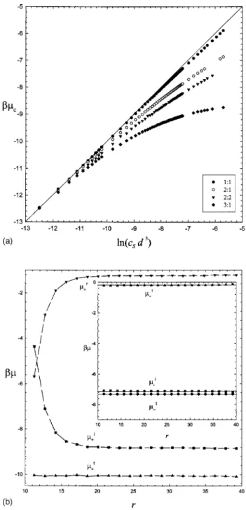
In order to determine the effective ion concentration, we have to know the reference relation between chemical poten-tial and salt concentration, 共cs兲, for various salt solutions. They can be obtained by MC simulations in a WS cell in the absence of the charged colloid, i.e., corresponding to pure salt solutions. Figure 1共a兲 shows the variation of  with ln csd3for simple z+: z−salt. Sincer⬍0 due to electrostatic
attraction, the counterion chemical potential is ⬍ln csd3 for high enough concentrations. The deviation from the ideal behavior is significant for multivalent salts and is most seri-ous for 3:1 salt. For a dilute solution of monovalent salt, since r共r=R兲⬵0, one has ⬵ln c共r=R兲d3. Therefore,
the effective ion concentration can also be estimated from the ion concentration at the cell boundary, ci*⬵ci共r=R兲. For multivalent salt, however, has to be calculated and Fig.
1共a兲is used to estimate ci*.
Figure 1共b兲 demonstrates typical distributions of ion concentration cid3, its residual chemical potential ir, and total chemical potential i for the addition of 3:1 salt in a dilute colloidal solution with Z = 100. Owing to electrostatic
attraction of the charged colloid, the trivalent counterion concentration c+共r兲 decays rapidly from the particle surface
to the boundary of the WS cell. It corresponds to the fast decay of the ideal chemical potential. On the contrary, the residual chemical potential is quickly increased with r. Nonetheless, the total chemical potential is essentially con-stant for all radial position r, as illustrated in Fig.1共b兲. Note that Widom’s method may be inaccurate for the +r calcula-tion at the concentrated region共in the vicinity of the charged particle兲 or at small N+共near the cell boundary兲. Evidently, in
the present case, the salt concentration is high enough and thereby the ion concentrations at the cell boundary cannot represent their effective concentrations. That is, c*has to be
FIG. 1.共a兲 The variation of the counterion chemical potentialcwith the
salt concentration csd3for various simple salts.共b兲 The typical variation of
the ideal共i兲, residual 共r兲, and total 共t兲 chemical potentials with the radial
position r for 3:1 salt with a = 10, R = 40, and Z = 80. The results for coion
determined from the relationship between the ion concentra-tion and its chemical potential in a pure salt soluconcentra-tion,共cs兲, as provided in Fig.1共a兲.
IV. RESULTS AND DISCUSSION
The effective charge of colloids in a dilute solution is thermodynamically defined based on ion chemical potential. It is closely related to the activity coefficient of macroion and can be reduced to the typical definition for binary elec-trolyte solutions. Similarly, the effective ion concentration in the colloidal solution is equivalent to the ionic activity and can be experimentally determined by potentiometry. As a result, for a salty dispersion, the effective charge of colloids can be obtained by using the electroneutrality condition if all effective ion concentrations are known. On the basis of spherical WS cell model, we perform MC simulations to evaluate the effective ion concentrations and thereby the ef-fective charge for colloidal dispersions with/without salt ad-dition. Besides monovalent salt, particular interests will be focused on the effect of multivalent counterion.
A. Salt-free colloidal solution
In a salt-free dispersion, the effective charge is propor-tional to the degree of ionization␣, as shown in Eqs.共6兲–共8兲. According to the partition function,␣ is a function of Z / zc,
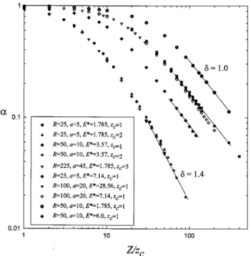
a /, and R/, where =zc2ᐉB.10 Figure 2 depicts the varia-tion of the charge ratio␣= Z*/ Z with the number of
counte-rions Z / zc for various combinations兵a,R,E*, zc其. As antici-pated, ␣ descends gradually from unity at small value of Z / zc but drops fast at large value of Z / zc. Under the same condition of 兵a/,R/其, data points of different combina-tions of 兵a,R,ᐉB, zc其 fall into a single curve. For example, the condition共R=50, a=10, ᐉB= 3.57, zc= 2兲 is equivalent to
共R=100, a=20, ᐉB= 28.56, zc= 1兲. For a given R/a and Z/zc, Fig. 2 discloses that Z* declines with increasing , which
depicts the characteristic length associated with Coulomb in-teraction. For instance, stronger Coulomb coupling due to lower dielectric constant leads to a smaller effective charge of colloid.
When Z / zc is large enough, it seems that the scaling relation is followed,␣⬃共Z/zc兲−␦with␦艌1. When the Cou-lomb coupling is weak, one has␦= 1 and thus Z*reaching a
constant for large enough Z. In other words, as the charge density of the colloid exceeds approximately a certain value, the counterions seem to condense on the sphere. This conse-quence is very similar to the so-called Manning condensation taking place along an infinitely long charged rod.19 On the other hand, as the Coulomb coupling is strong, the exponent ␦ is greater than unity and therefore Z*⬃1/共Z␦−1兲. For ex-ample, one has ␦⯝1.4 for the condition R/=14.0 and a /=2.8. This consequence discloses the fact that the effec-tive charge is essentially decreased with increasing intrinsic charge. Although the intrinsic charge is very large, the Cou-lomb attraction strongly favors “counterion condensation” and effectively leads to a weakly charged particle. As shown in Fig.2, the charged sphere possesses an effective charge of about Z*⯝2 for Z/z
c= 100. Note that for␦⬎1, there exists a maximum Z* as Z is increased owing to the competition
between counterion entropy and electrostatic attraction.10
B. Effective ion concentrations„activity coefficient…
The effective ion concentration is determined by the ion chemical potential or activity coefficient according to Fig.
1共a兲. For monovalent salt, it can be evaluated from the ion concentration at the WS cell boundary as well. Since the coion is repelled from the charged sphere, one expects that its effective concentration is greater than its intrinsic concen-tration, i.e., c−*⬎c−. However, due to the small volume frac-tion associated with the double layer region and the electro-static contribution to the residual chemical potential, the effective coion concentration is essentially equal to its intrin-sic concentration, i.e., c−*/ c−=␥+⬵1. Figure 3共a兲
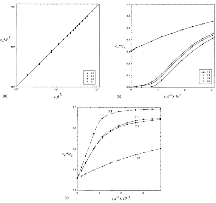
demon-strates the variation of the effective coion concentration with its intrinsic concentration for various z+: z− added salts at R
= 40, a = 10, and Z = 100. All data points fall at the straight line with the slope unity. That is, the effective coion concen-tration in a salty colloidal dispersion can be simply estimated from the added salt concentration.
Since c−*⬵c−, the effective counterion concentrations
play an important role in determining the effective charge. Figure3共b兲shows the variation of the effective concentration of added counterion 共c+*/ c+兲 with the added salt
concentra-tion cs= c+, while Fig. 3共c兲 illustrates the variation of the
effective concentration of original counterion 共cc
*
/ cc兲 with the added salt concentration. Note that for R = 40, cid3 = 10−4 corresponds to 2.6 mM and ccd3= 3.73⫻10−4 for Z = 100. As indicated in Figs.3共b兲 and3共c兲, the effective con-centrations of both added counterion共c+*兲 and original coun-terion共cc*兲 rise with increasing cs. Although the increment of
FIG. 2. The variation of the charge ratio Z*/ Z with Z / z
cfor a salt-free
dispersion with various combinations of兵R,a,E*, z
c其. The exponent␦is for
c+* with increasing cs is anticipated, the fact that c+ *⬍c
+
re-veals that some of the added counterions are “condensed” on the colloid.
For monovalent salt, there is actually no difference be-tween original and added counterions in terms of Coulomb interaction. As a result, the activity coefficients for original and added counterions should be the same,
␥+= c+* c+ =cc * cc =␥c. 共15兲
Comparison between Figs.3共b兲and3共c兲for 1:1 salt confirms the validity of Eq. 共15兲. For example, as c+d3→0, c+*/ c+
⬵cc
*
/ cc⬇0.31. The monovalent counterion may play two roles: replacement and “condensation.” First, some original condensed counterions are replaced by added counterions. Secondly, some added counterions are attracted to the colloid
because it still possesses significant effective charge. If the first mechanism dominates, then monovalent salt addition has an insignificant influence on the effective charge. If Z*is independent of cs, then one must have ␥+= 1 according to
Eqs.共10兲and共15兲. Obviously, this result disagrees with Eq.
共15兲 because of ␥c⬍1. The above analysis reveals that the second mechanism plays an important role. Since some of the added counterions are attracted to the colloid, one ex-pects that the effective charge may decline due to monova-lent salt addition.
For multivalent salt, the added counterions共multivalent兲 have stronger Coulomb attraction than the original counteri-ons 共monovalent兲 and it can be roughly classified into two regimes. For csd3ⱗ10−4, c+
*
/ c+is close to zero as shown in
Fig.3共b兲and cc
*
/ ccgrows rapidly as illustrated in Fig.3共c兲. When the added salt concentration is low, most of the
mul-FIG. 3. 共a兲 The effective coion concentration c−* is plotted against the intrinsic coion concentration c
−for various multivalent salts.共b兲 The effective
concentration of added counterion, c+*/ c+共activity coefficient兲, is plotted against the intrinsic counterion concentration c+for various multivalent salts. The
solid curves are drawn to guide the eyes. 共c兲 The effective concentration of original counterion, cc
*/ c
c 共activity coefficient兲, is plotted against the salt
tivalent counterions are accumulated in the vicinity of the colloid. This leads to the release of the monovalent counte-rions. On the other hand, for csd3ⲏ10−4, c+*/ c+ is increased
with increasing cs, but cc*/ ccseems to approach an asymptote close to unity. This result reveals that a small amount of monovalent counterions is always in the neighborhood of the colloid. For high salt concentration, most of monovalent counterions are already released and multivalent counterions left in the bulk solution rises with added salt concentration. Nonetheless, just like addition of monovalent salt, a part of the newly added multivalent counterions continues to be at-tracted to the colloid. Therefore, salt addition leads to reduc-tion of the effective charge.
C. Effective charge
Once the effective ion concentrations are obtained, the effective charge associated with a colloid can be determined by Eq. 共10兲 based on the electroneutrality condition. For a given R and a, the effective charge is a function of intrinsic charge and added salt concentration, i.e., Z*共Z,cs兲. Figure
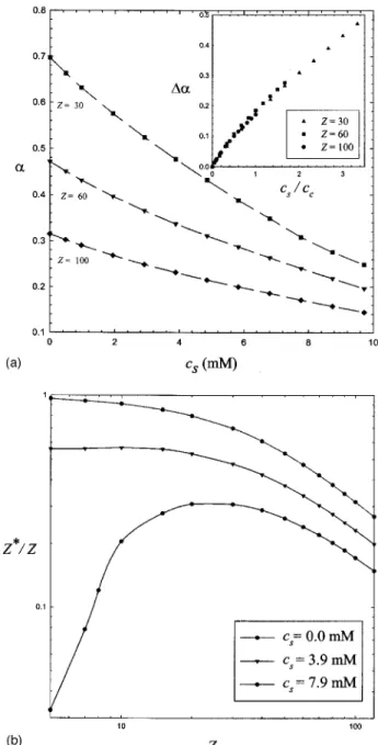
4共a兲shows the variation of the charge ratio Z*/ Z with the added 1:1 salt concentration for a specified Z with R = 40 and a = 10. Evidently, the effective charge declines with increas-ing cs. The effective charge of a colloid represents a conse-quence of the competition between Coulomb attraction and counterion entropy. Our simulation results indicates that when monovalent salt is added, the loss of counterion en-tropy is responsible for the decrease of the effective charge. Moreover, the counterion fluctuation-correlation effect may provide additional attraction between counterions and col-loids. Figure4共a兲also shows that for a given amount of salt addition, the effect of salt addition on Z*is more significant
for a colloid with smaller Z than for one with larger Z. Since a colloid with larger intrinsic charge has higher free counter-ion concentratcounter-ion, one expects that more amount of salt is required to provide added counterions, which can neutralize the particle charge. Thus the extent of the change of the charge ratio,⌬␣, can be assumed as a function of the ratio of added salt concentration to the intrinsic counterion concen-tration, cs/ cc共or cs/ Z兲. As shown in the inset of Fig.4共a兲, the data points for three different values of Z fall into a single curve, confirming this relationship. Note that ⌬␣=␣共cs= 0兲 −␣共cs兲 with ␣= Z*/ Z and the concentration range of added salt in Fig. 4共a兲 corresponds to csⱗcc. The fact that the change in␣ grows with cs/ Z instead of cs indicates that at high enough salt concentration, one may have ␣共Z1兲
⬍␣共Z2兲 for Z1⬍Z2 even though ␣0共Z1兲⬎␣0共Z2兲, where ␣0
=␣共cs= 0兲. Moreover, the approximately linear relation be-tween⌬␣and cs/ ccat higher values of cs/ ccreveals that the effective charge may approach zero essentially at high enough salt concentration.
Figure4共b兲 illustrates the variation of Z*/ Z with the
in-trinsic charge for a given cs with R = 40 and a = 10. In a salt-free colloidal solution 共cs= 0兲, the charge ratio Z*/ Z is monotonically decreased from unity toward zero. This is simply because of the increase in Coulomb attraction and the decrease in counterion entropy as Z grows. Unlike the salt-free case, there exists a maximum value of the charge ratio␣
under a constant salt concentration. It can also be attributed to the competition between Coulomb attraction 共increasing Z兲 and counterion entropy 共decreasing Z兲. There are two lim-its. 共i兲 For ccⰇcs, the colloidal dispersion behave just like the salt-free case. As a result,␣ declines with increasing Z. 共ii兲 For ccⰆcs, decreasing Z is equivalent to increasing cs/ Z, which magnifies the effect of salt addition. Consequently,␣ declines with decreasing Z. The compromise between these two effects results in␣maxfor a specified cs.
Addition of multivalent salt can reduce the effective charge much more efficiently than addition of monovalent salt. As shown in Fig. 5, the effective charge is plotted against the salt concentration for various multivalent salts with Z = 100共cc⯝10 mM兲. The effective charge drops very
FIG. 4. 共a兲 The variation of the charge ratio␣ with the monovalent salt concentration csfor colloid with different values of intrinsic charge Z. The
dotted curves are drawn to guide the eyes. The data points are replotted in the inset for⌬␣=␣0 −␣vs cs/ cc.共b兲 The variation of the charge ratio Z*/ Z
with the intrinsic charge Z for different monovalent salt concentrations. The solid curves are drawn to guide the eyes.
quickly upon addition of 3:1 salt. For example, the effective charge becomes Z*/ Z⬇0.02 for 3 mM 3:1 salt, but is still Z*/ Z⬇0.14 for 10 mM 1:1 salt. According to the PB theory,
the effect of salt addition is usually understood in terms of the ionic strength, I =共c+z+2+ c−z−2兲/2. If the effectiveness of
reducing Z* is proportional to the ionic strength, then the
equivalent concentrations are 6:4:3:1 for 3:1, 2:2, 2:1, and 1:1 salts, respectively, for the same salt concentration. That is,
␣共zc兲 ⬇␣0−⌬␣共zc= 1兲
冋
I共zc兲
I共zc= 1兲
册
for a specified cs. This simple model would predict that
Z*/ Z⯝0 for 3 mM 3:1 salt based on the result of
monova-lent salt. It agrees approximately with the simulation result. This model also predicts that 2:2 salt is more effective than 2:1 salt. This result is inconsistent with our simulation result, as illustrated in Fig.5. Nonetheless, the differences between these two salts are quite small.
The results of monovalent salt reveal that the reduction of Z* by salt addition is more significant for colloids with
lower Z. In order to have the same extent of ␣ reduction 共⌬␣兲, the added salt concentration for Z=60 must be twice that for Z = 30. It is anticipated that␣for Z = 30 will be lower than␣for Z = 60 eventually as the salt concentration contin-ues increasing. In the dilute limit, however, it is difficult to observe this phenomenon simply by addition of a monova-lent salt. With the addition of 3:1 salt, this effect is clearly confirmed in Fig.6 for Z = 30, 60, 100. Despite the fact that the charge ratio for Z = 30 is the highest, ␣0⯝0.7, it decays
rapidly with cs and becomes lowest at about cs⬇1 mM. In other words, for a given amount of salt, the influence on the effective charge decreases with increasing intrinsic charge. The relation Z*共Z,cs兲 can be reexpressed as ⌬␣共cs/ cc兲, as
demonstrated in the inset of Fig. 4共a兲 for monovalent salt. For weak Coulomb coupling, an approximately linear rela-tion is observed. However, as shown in the inset of Fig. 6, addition of multivalent salt results in significant deviation from the weak-coupling behavior. Because of the strong at-traction between multivalent counterion and colloid, ⌬␣ is increased rapidly from the weak-coupling to strong-coupling regimes. While an approximately linear increase is displayed in the former regime,⌬␣approaches a constant,⌬␣⯝␣0, in the latter regime.
A colloidal dispersion can be kinetically stabilized by electrostatic repulsions. The accumulation of counterions around the charged particle forms the diffuse layer of the electric double layer.20 The overlap of the electric double layers associated with two colloids leads to repulsion. It is generally accepted that for a colloid with constant surface charge, salt addition leads to the decrease of the thickness of the diffuse layer共Debye screening length−1兲 and therefore
weakens the electrostatic repulsion between two colloids. According to the present study, the reduction of the electro-static repulsion due to salt addition can also be explained by the decrease of the effective charge associated with the col-loid. Moreover, the addition of multivalent salt is able to lessen the effective charge very efficiently. Consequently, the van der Waals attraction between two colloids can overcome the electrostatic repulsion easily and results in colloidal ag-gregation. Precipitation of colloids due to addition of multi-valent salt is frequently observed experimentally.
The effective charge is often determined experimentally by electrophoresis. The generic approximate expression re-lating the electrophoretic mobility of a protein to its effective charge is E⬃Z* for the same particle size.21 In accordance with electrokinetic phenomena, the electrophoretic mobility Eassociated with a charged particle is proportional to its
FIG. 5. The variation of the charge ratio␣with the salt concentration csfor
a = 10, R = 40, and Z = 100. The simple added salts include 2: 1, 2: 2, and 3:
1 multivalent counterions. The dotted curves are drawn to guide the eyes.
FIG. 6. The variation of the charge ratio␣with the concentration of 3: 1 salt, cs, for colloid with different values of intrinsic charge Z. The solid lines
are drawn to guide the eyes. The data points are redrawn in the inset for ⌬␣=␣0−␣vs cs/ Z.
potential,22which is approximately equivalent to the surface potential ⌿s. As a result, E⬃⌿s. The aforementioned analysis indicates that Z*⬃⌿
s. Note that such a definition of effective charge is based on transport properties, instead of thermodynamics. Figure 7 shows that the influence of salt addition on the surface potential for Z = 100. the qualitative behavior of⌿s is quite similar to Z* based on ion chemical potential. The absolute value of the surface potential declines with increasing cs. The effect of multivalent salt is much more significant than monovalent salt. Nevertheless, the fact that Z1*/ Z2*⫽⌿s,1/⌿s,2 indicates that different definitions of effective charge may give different values of Z*. According
to the linearized PB theory, the surface potential is related to the ionic strength by ⌿s⬃Z/共1+a兲. Therefore, ␣⬃共1 +a兲−1due to Z*= Z␣共cs兲. Since=共8ᐉBI兲1/2, the effective charge based on electrophoretic mobility also declines with increasing cs and is reduced very efficiently by addition of multivalent salt.
It is important to compare the effective charge based on ion chemical potential with that based on far-field behavior. Within the PB theory, the latter has been obtained by using the analytic solutions for a sphere.23,24 It is shown that at high enough intrinsic charge, nonlinear effects come into play and the effective charge is dramatically affected by salt addition.23 Moreover, the effective charge depends on elec-trolyte asymmetry besides the Debye length. For a given value of the ionic strength, the effective charge may differ by a factor exceeding 2 between 2:1 and 1:2 cases.24 Those phenomena agree qualitatively with our findings. However, Z* based on far-field behavior grows with increasing salt
concentration. For example, in the limit of diverging intrinsic charge with monovalent salt, the effective charge can be sim-ply expressed by23
ᐉB
a Z
*= 4a + 6 + O
冉
1a
冊
.Note that it is the exact expansion of the correct result in the limit of largea. This consequence is opposite to that based on chemical potential, which declines with increasing cs. Evidently, the definition based on far-field behavior is unable to explain the determination of Z*by electrophoresis, which
decays with cs.
21
V. CONCLUSION
In a solution containing charged particles, counterions are always accumulated in the vicinity of the surface of the charged particle with intrinsic charge Z. The effective charge Z*is therefore invoked to represent the physical behavior of
such a highly charged colloidal dispersion. The value of the effective charge changes with its definition. In other words, it is model dependent. Unfortunately, a thermodynamic defini-tion of Z*, which can also be experimentally measurable, is
generally lacking. In this study, we propose an operational definition of the effective charge, which is thermodynami-cally well defined and can be determined by potentiometry.7 On the basis of this definition, we are able to investigate the effect of multivalent salt addition on the effective charge of a dilute colloidal dispersion.
Although the ion concentrations ciare not uniform in the solution due to the presence of the charged particles, their chemical potentials are uniform everywhere. Therefore, on the basis of ion chemical potential, one can define an effec-tive ion concentration ci
*
, which can be experimentally mea-sured by ion-selective electrode. Note that ci
*
reduces to ciin the absence of charged colloids. This definition is essentially equivalent to the ionic activity coefficient 共␥i= ci
*
/ ci兲 with the pure salt solution as the reference state. Once all the effective ion concentrations are obtained, the effective charge associated with the charged particle can then be de-termined by the global electroneutrality condition. In fact, the effective charge denotes the activity coefficient associ-ated with the colloid, ␥p= Z*/ Z. Our approach is consistent with the conventional thermodynamic theory for a solution of a strong electrolyte. Applying such a definition to a salt-free colloidal solution yields a result similar to that of an unsymmetrical electrolyte solution. For example, consider small charged particles with valency Z = −4 and counterions with z = + 1. If one regards them as a colloid solution and applies current definition, then the result is consistent with that regarding them as a strong electrolyte solution 共activity coefficient兲.
In order to explore the influence of adding multivalent salt, Monte Carlo simulations are performed in a spherical Wigner-Seitz cell to obtain the effective charge of the col-loid. In terms of the charge ratio ␣= Z*/ Z, the effects of
added salt concentration, counterion valency, and particle charge are examined. The effective charge declines with in-creasing salt concentration and the multivalent salt is much more efficient in reducing the effective charge of the colloi-dal solution. Moreover, the extent of effective charge reduc-tion is decreased with increasing intrinsic charge for a given concentration of added salt. Those results are qualitative
con-FIG. 7. The dimensionless surface potential⌿s=esis plotted against the
salt concentration cs for various multivalent salts with Z = 100. The solid
sistent with experimental observations by electrophoresis. We have investigated dilute systems containing particle size of about 4 nm共a=10兲 with surface charge density of about 0.1 C / m2共Z⬃100兲. They correspond to the micellar or
pro-tein solution. Nonetheless, our results can be generally ap-plied to typical colloidal dispersions with much larger a and Z.
ACKNOWLEDGMENTS
This research is supported by the National Council of Science of Taiwan under Grant No. NSC-95-2221-E-008-146-MY3. Computing time provided by the National Center for High-Performance Computing of Taiwan is gratefully ac-knowledged.
1S. Alexander, P. M. Chaikin, P. Grant, G. J. Morales, and P. Pincus, J.
Chem. Phys. 80, 5776共1984兲.
2E. Trizac, L. Bocquet, and M. Aubouy, Phys. Rev. Lett. 89, 248301
共2002兲.
3R. D. Groot, J. Chem. Phys. 95, 9191共1991兲.
4M. J. Stevens, M. L. Falk, and M. O. Robbins, J. Chem. Phys. 104, 5209
共1996兲.
5J. M. Roberts, J. J. O’Dea, and J. G. Osteryoung, Anal. Chem. 70, 3667
共1998兲.
6V. K. Aswal and P. S. Goyal, Phys. Rev. E 67, 051401共2003兲.
7C. C. Hsiao, T.-Y. Wang, and H.-K. Tsao, J. Chem. Phys. 122, 144702
共2005兲.
8R. D. Void and M. J. Void, Colloid and Interface Chemistry
共Addison-Wesley, Reading, MA, 1983兲.
9V. Sanghiran and K. S. Schmitz, Langmuir 16, 7566共2000兲.
10W. L. Hsin, T.-Y. Wang, Y.-J. Sheng, and H.-K. Tsao, J. Chem. Phys. 121, 5494共2004兲.
11M. Muthukumar, J. Chem. Phys. 120, 9343共2004兲.
12T.-Y. Wang, T.-R. Lee, Y.-J. Sheng, and H.-K. Tsao, J. Phys. Chem. B 109, 22560共2005兲.
13D. A. McQuarrie, Statistical Mechanics 共Happer & Row, New York,
1976兲.
14G. V. Ramanathan, J. Chem. Phys. 88, 3887共1988兲. 15L. Belloni, Colloids Surf., A 140, 227共1998兲.
16M. Deserno and C. Holm, Electrostatic Effects in Soft Matter and
Bio-phyiscs共Kluwer Academic, Netherlands, 2001兲, p. 27; H. Wennerström,
B. Jönsson, and P. Linse, J. Chem. Phys. 76, 4665共1982兲.
17Y.-J. Sheng and H.-K. Tsao, Phys. Rev. Lett. 87, 185501共2001兲; Phys.
Rev. E 66, 040201共R兲 共2002兲; C.-H. Ho, H.-K. Tsao, and Y.-J. Sheng, J. Chem. Phys. 119, 2369共2003兲.
18D. Frenkel and B. Smit, Understanding Molecular Simulation
共Aca-demic, New York, 1996兲.
19G. S. Manning, J. Chem. Phys. 51, 924共1969兲.
20E. J. W. Verwey and J. T. G. Overbeek, Theory of the Stability of
Lyo-phobic Colloids共Elsevier, Amsterdam, 1948兲.
21J. Gao, F. A. Gomez, R. Härter, and G. W. Whitesides, Proc. Natl. Acad.
Sci. U.S.A. 91, 12027共1994兲.
22R. F. Probstein, Physicochemical Hydrodynamics: An Introduction
共Wiley, New York, 1994兲.
23M. Aubouy, E. Trizac, and L. Bocquet, J. Phys. A 36, 5835共2003兲. 24G. Téllez and E. Trizac, Phys. Rev. E 70, 011404共2004兲.