Incremental Maintenance of Generalized
Association Rules under Taxonomy
Evolution
Ming-Cheng TsengInstitute of Information Engineering, I-Shou University, Kaohsiung 840, Taiwan. E-mail: [email protected]
Wen-Yang Lin
Department of Computer Science and Information Engineering, National University of Kaohsiung, Kaohsiung 811, Taiwan. E-mail: [email protected]
Rong Jeng
Department of Information Management, I-Shou University, Kaohsiung 840, Taiwan. E-mail: [email protected] Correspondence to: Wen-Yang Lin, Department of Computer Science and Information Engineering, National University of Kaohsiung, Kaohsiung 811, Taiwan. E-mail: [email protected]
Abstract
Mining association rules from large databases of business data is an important topic in data mining. In many applications, there are explicit or implicit taxonomies (hierarchies) over the items, so it may be more useful to find associations at different levels of the taxonomy than only at the primitive concept level. Previous work on the mining of generalized association rules, however, assumed that the taxonomy of items are kept unchanged, disregarding the fact that the taxonomy might be updated as new transactions are added into the database over time. Under this circumstance, how to effectively update the discovered generalized association rules to reflect the database change with the taxonomy evolution is a crucial task. In this paper, we examine this problem and propose two novel algorithms, called IDTE and IDTE2, which can incrementally update the discovered generalized association rules when the taxonomy of items is evolved with new transactions. Empirical evaluations show that our algorithms can maintain their performance even in large amounts of incremental transactions and high degree of taxonomy evolution, and is faster than applying the contemporary generalized association mining algorithms to the whole updated database.
1. Introduction
Mining association rules from large databases of business data, such as transaction records, is a significant topic in the research on data mining [1][2]. An association rule is an expression of the form X Y, where X and Y are sets of items. Such a rule reveals that transactions in the database containing items in X tend to also contain items in Y, and the probability, measured as the fraction of transactions containing X that also contain Y, is called the confidence of the rule. The support of the rule is the fraction of the transactions that contain all items in both X and Y. For an association rule to be valid, the rule should satisfy a user-specified minimum support, called ms, and minimum confidence, called mc, respectively. The problem of mining association rules is to discover all association rules that satisfy ms and mc.
In many applications, there are explicit or implicit taxonomies (hierarchies) over the items, so it may be more useful to find associations at different levels of the taxonomy than only at the primitive concept level [3][4]. For example, consider the taxonomy of items in Figure1,where“PC”denotes“PersonalComputer”,“PDA” denotes “PersonalDigitalAssistance”and “IBM TP”isa kind of Notebook. It is likely that the association rule,
Systemax V HP LaserJet (Support 20%, Confidence100%),
does not hold when the minimum support is set to 30%, but the following association rule may be valid, Desktop PC HP LaserJet.
To the best of our knowledge, most work to date on mining generalized association rules required the taxonomy to be static [3][4][5][6], ignoring the fact that the taxonomy may change as time passes and new transactions are continuously added into the original database [7]. For example, items corresponding to new products must be added into the taxonomy, and their insertion would further introduce new classifications if they are of new types. On the other hand, items and/or their classifications will also be abandoned if they are no longer produced. All of these changes would reshape the taxonomy and in turn would invalidate previously discovered generalized association rules and/or introduce new ones, not to mention the changes caused by the transaction update to the database. Under these circumstances, it is important to find a method to effectively update the discovered generalized association rules.
PDA HP LaserJet
MITAC Mio ACER N Desktop PC
PC
IBM TP
Systemax V Sony VAIO
In this paper, we examine the problem of maintaining the discovered generalized association rules when new transactions are added to the original database along with taxonomy evolution. We give a formal problem description and clarify the situations for a taxonomy updating in Section 2.
A straightforward strategy to deal with this problem is to apply one of the generalized association mining methods to the whole database from scratch to find associations that reflect the most recent associations. This approach, however, has the following disadvantages:
1. The process of generating frequent itemsets is very time-consuming.
2. It is not cost-effective because the discovered frequent itemsets are not reused.
A more realistic and cost-effective alternative is to employ an association mining algorithm to generate the initial association rules, and when updates to the source database and taxonomy occur, apply an updating method to re-build the discovered rules. The challenge becomes that of developing an efficient updating algorithm to facilitate the overall mining process. This problem is nontrivial because updates to the database and taxonomy not only can reshape the concept hierarchy and the form of generalized items, but also may invalidate some of the discovered association rules, thus turning previous weak rules into strong ones, and generating important new rules.
In this paper, we propose two algorithms, called IDTE (Incremental Database and Taxonomy Evolution) and IDTE2, for mining the generalized frequent itemsets. These algorithms are capable of effectively reducing the number of candidate sets and database rescanning, and so they can efficiently update the generalized association rules. A detailed description of the IDTE and IDTE2 algorithms is given in Section 3.
In Section 4, we use synthetic data to evaluate the performance of the proposed IDTE and IDTE2 with two leading generalized association mining algorithms, Cumulate and Stratify [4]. A remark on previous related work is presented in Section 5. Finally, we summarize our work and propose future investigations in Section 6.
2. Problem statement
In real business applications the databases are changing over time, with new transactions (e.g., new types of items) continuously added and outdated transactions (e.g., abandoned items) deleted. Thus the taxonomy that represents the classification of items must also evolve to reflect such changes. This implies that if the updated database is processed afresh, some of the previously discovered associations might be invalid and some undiscovered associations should be generated. That is, the discovered association rules must be updated to reflect the new circumstance. Analogous to mining associations, this problem can be reduced to updating the frequent itemsets.
2.1. Problem description
Consider the task of mining generalized frequent itemsets from a given transaction database DB with the item taxonomy T. In the literature, although different proposed methods have different strategies for implementation, the main process involves adding to each transaction the generalized items in the taxonomy [3][4][5][6]. For this reason, we can view the task as mining frequent itemsets from the extended database ED, the extended version of DB, by adding to each transaction the ancestors of each primitive item in T. We use LED to denote the set of newly discovered frequent itemsets.
Assume that the minimum support constraint ms is kept constant. Now let us consider the situation when new transactions in db are added to DB, and the taxonomy T is changed into a new one, T . Following the previous paradigm, we can view the problem as follows. Let ED and ed denote the extended version of the original database DB and incremental database db, respectively, by adding to each transaction the generalized items in T . Further, let UE be the updated extended database containing ED and ed , i.e., UE ED + ed . The problem of updating LED when new transactions db are added to DB, and T is changed into T , is equivalent to finding the set of frequent itemsets in UE , denoted as L .UE
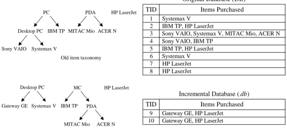
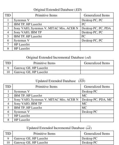
For illustration, consider an original database with the old item taxonomy and an incremental database with the new item taxonomy in Figure 2. Assume that primitive item “Sony VAIO”and generalized item “PC”are deleted from the “PC”group, and new primitive item “Gateway GE”isinserted into its top generalized item “MC”. The corresponding extended databases, including ED, ed, ED , and ed , are shown in Figure 3.
2.2. Situations for taxonomy evolution and frequent itemset update
By intuition, both the taxonomy evolution and its effect on previously discovered frequent itemsets are more complex than those for data updates because the taxonomy evolution induces item rearrangement: once an item, primitive or generalized, is reclassified into another category, all of its ancestors (generalized items) in both the old and the new taxonomy are affected. In this subsection, we describe different situations for taxonomy evolution, and clarify the essence of frequent itemset updates for each type of taxonomy evolution.
PDA HP LaserJet
Desktop PC PC
IBM TP MITAC Mio
Systemax V Sony VAIO
ACER N
Old item taxonomy
Original Database (DB) 1 3 2 Systemax V IBM TP, HP LaserJet
TID Items Purchased
Sony VAIO, Systemax V, MITAC Mio, ACER N
5 4
IBM TP, HP LaserJet Sony VAIO, IBM TP
6 Systemax V 7 8 HP LaserJet HP LaserJet HP LaserJet Desktop PC Systemax V Gateway GE MC IBM TP ACER N PDA MITAC Mio New item taxonomy
Incremental Database ( db) 9
10
Gateway GE, HP LaserJet Gateway GE, HP LaserJet
TID Items Purchased
Figure 2. Example of original database DB with old item taxonomy and incremental database db with new item taxonomy.
According to our observation, there are four basic types of item updates that will cause taxonomy evolution: 1. Item insertion: New items are added to the taxonomy.
2. Item deletion: Obsolete items are removed from the taxonomy.
3. Item renaming: Items are renamed for certain reasons, such as error correction, product promotion, etc. 4. Item reclassification: Items are reclassified into different categories.
Note that hereafter the term “item”refers to a primitive or a generalized item. In the following, we elaborate each type of evolution.
Type 1: Item insertion. There are different strategies to handle this type of update operation, depending on whether the inserted item is a primitive or a generalized item.
When the new inserted item is primitive, we do not have to process it until an incremental database update containing that item occurs. This is because the new item does not appear in neither the original database, nor the discovered associations. However, if the new item is a generalization, then the insertion will affect the discovered associations since a new generalization often incurs some item reclassification.
Original Extended Database (ED) 1 3 2 Systemax V IBM TP, HP LaserJet
TID Primitive Items
Sony VAIO, Systemax V, MITAC Mio, ACER N 5
4
IBM TP, HP LaserJet Sony VAIO, IBM TP 6 Systemax V 7 8 HP LaserJet HP LaserJet Desktop PC, PC PC Desktop PC, PC, PDA Desktop PC, PC Desktop PC, PC PC Generalized Items
Original Extended Incremental Database ( ed)
9 10
Gateway GE, HP LaserJet Gateway GE, HP LaserJet
TID Primitive Items Generalized Items
Updated Extended Database
1 3 2
Systemax V IBM TP, HP LaserJet
TID Primitive Items
Sony VAIO, Systemax V, MITAC Mio, ACER N 5
4
IBM TP, HP LaserJet Sony VAIO, IBM TP 6 Systemax V 7 8 HP LaserJet HP LaserJet Desktop PC MC Desktop PC, PDA, MC MC Desktop PC MC Generalized Items ) (ED ) (ed
Updated Extended Incremental Database
9 10
Gateway GE, HP LaserJet Gateway GE, HP LaserJet
TID Primitive Items
Desktop PC Desktop PC
Generalized Items
Figure 3. The corresponding extended databases: ED, ed, ED , and ed .
Example 1. Figure 4 shows this type of taxonomy evolution. In Figure 4(a), a new primitive item “ASUS W”is inserted into the generalized item “PC”. Because the new item “ASUS W”does not appear in the original transactions, and so is not in the original set of frequent itemsets, we do not have to process it until there is an incremental database update. Next, we consider the case of a new generalization insertion. In Figure 4(b), a generalized item “Desktop PC”is inserted as a child of the generalized item “PC”,anditems “Sony VAIO”and “Systemax V” arereclassified to the new generalization, “Desktop PC”. Since items “Sony VAIO” and “Systemax V”already exist in the original database, we must process them to update the generalized frequent itemsets.
PDA HP LaserJet PC
IBM TP MITAC Mio Systemax V
Sony VAIO ACER N
ASUS W
PDA HP LaserJet PC
IBM TP MITAC Mio ACER N
Systemax V Sony VAIO
Desktop PC
(a) (b)
Figure 4. Example of taxonomy evolution caused by item insertion. The inserted new item is: (a) primitive; (b) generalized.
Type 2: Item deletion. Unlike the case of item insertion, the deletion of a primitive item from the taxonomy would incur a problem of inconsistency. In other words, if there is no transaction update to delete the occurrence of that item, then the refined item taxonomy will not conform to the database. An outdated item continues to appear in the transaction of interest.To simplify this problem, we assume that the updated extended database is always consistent with the evolution of the taxonomy. Additionally, the removal of a generalization may also lead to item reclassification. Therefore, we also have to deal with the situation caused by item deletion.
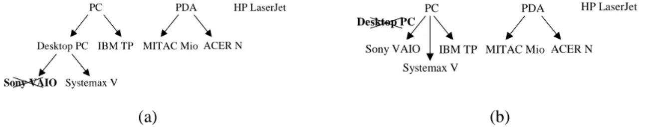
Example 2. Figure 5 shows this type of taxonomy evolution, where Figure 5(a) illustrates the deletion of the primitive item “Sony VAIO”, and Figure 5(b) demonstrates the removal of the generalized item “Desktop PC” and the reclassification of “Sony VAIO”and “Systemax V”to “PC”.
PDA HP LaserJet
Desktop PC PC
IBM TP MITAC Mio
Systemax V
ACER N
Sony VAIO
PDA HP LaserJet
PC
IBM TP MITAC Mio Systemax V
Sony VAIO ACER N
Desktop PC
(a) (b)
Figure 5. Example of taxonomy evolution caused by item deletion: (a) primitive; (b) generalized.
Type 3: Item renaming. Items may be renamed for many reasons such as error correction, product promotion, or just for novelty. When items are renamed, we do not have to process the database since the processing codes of the renamed items are the same. Instead, we just replace the discovered frequent itemsets and the association rules with the new names.
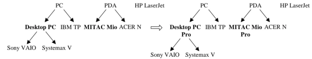
Example 3. Figure 6 shows this type of taxonomy evolution, where the generalized item “Desktop PC” is renamed to “Desktop PC Pro”, and the primitive item “MITAC Mio”is renamed to “MITAC Mio Pro”.
PDA HP LaserJet
Desktop PC
PC
IBM TP MITAC Mio
Systemax V Sony VAIO ACER N PDA HP LaserJet Desktop PC Pro PC
IBM TP MITAC Mio
Pro
ACER N
Systemax V Sony VAIO
Figure 6. Example of taxonomy evolution caused by item renaming.
Type 4: Item reclassification. Among all types of taxonomy updates this is the most far-reaching operation. Once an item, primitive or generalized, is reclassified into another category, all of its ancestors (generalized items) in the old as well as the new taxonomy are affected. That is, the supports of these affected generalized items must be recounted, as are the frequent itemsets containing any one of the affected generalized items.
Example 4. Consider Figure 7. A new group “MC” denoting “Mobile Computer”is added along with the reclassification of “IBM TP”and “PDA”to “MC”.Therefore,theshifted item “IBM TP” willchangethesupport count of the generalized items“PC”,and “MC”,andalso affect the support count of any itemsets containing “PC”or“MC”.
HP LaserJet Desktop PC
Systemax V
Sony VAIO IBM TP
ACER N PDA MITAC Mio MC PDA HP LaserJet Desktop PC PC
IBM TP MITAC Mio
Systemax V Sony VAIO
ACER N
3. The proposed algorithms
Two algorithms for updating discovered frequent itemsets under incremental database update and taxonomy evolution, called IDTE and IDTE2, are proposed. We first introduce the basic paradigm, and then detail the process of each algorithm.
3.1. Algorithm IDTE 3.1.1 Basic paradigm
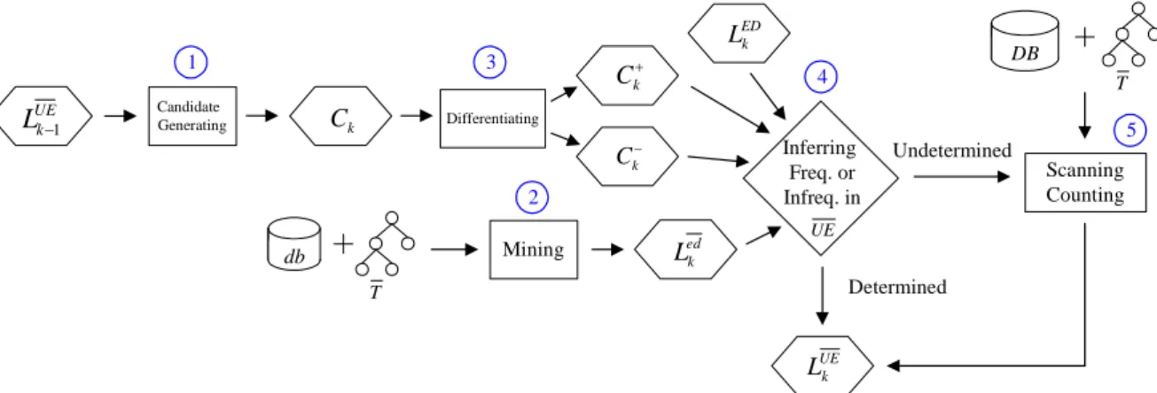
A straightforward way to find updated generalized frequent itemsets would be to run any of the algorithms for finding generalized frequent itemsets, such as Cumulate and Stratify [4], on UE . This simple way, however, ignores some of the discovered frequent itemsets are not affected by incremental update and/or taxonomy evolution; that is, these itemsets survive in the taxonomy evolution and remain frequent in the updated database UE . If we can identify the unaffected itemsets, then we can avoid unnecessary computations in counting their supports. In view of this, we decided to adopt the Apriori-based maintenance framework depicted in Figure 8.
ED k L Candidate Generating Ck Differentiating k C k C Mining Inferring Freq. or Infreq. in UE UE k L Determined Undetermined T DB db T ed k L 1 2 3 4 5 Scanning Counting UE k L1
Figure 8. Proposed Apriori-based framework for updating the frequent k-itemsets.
Each pass of mining the frequent k-itemsets involves the following main steps: 1. Generate candidate k-itemsets Ck.
2. Scan the incremental database db with the new taxonomy T to find ed k L . 3. Differentiate in Ckthe affected itemsets (C ) from the unaffected ones (k
k C ).
4. Incorporate LEDk , ed k L , C , andk k
C to determine whether a candidate itemset is frequent or not in the resulting database UE .
5. Scan DB with T , i.e., ED , to count the supports of itemsets that are undetermined in Step 4.
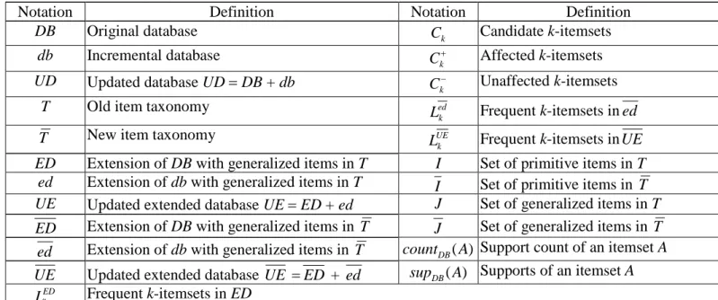
In summary, our approach is to differentiate the unaffected itemsets by the taxonomy evolution from the affected ones, and then use them to reduce the work spent on support counting of itemsets. Below, we first elaborate on each of the kernel steps, i.e., Steps 3 and 4, and then present a description of algorithm IDTE and illustrate its execution with a simple example. The notation that will be used is summarized in Table 1.
Table 1. Summary of the notation used in IDTE.
Notation Definition Notation Definition
DB Original database Ck Candidate k-itemsets
db Incremental database
k
C Affected k-itemsets UD Updated database UDDB + db Ck Unaffected k-itemsets
T Old item taxonomy ed
k
L Frequent k-itemsets in ed
T New item taxonomy UE
k
L Frequent k-itemsets inUE ED Extension of DB with generalized items in T I Set of primitive items in T
ed Extension of db with generalized items in T I Set of primitive items in T UE Updated extended database UEED + ed J Set of generalized items in T ED Extension of DB with generalized items in T J Set of generalized items in T ed Extension of db with generalized items in T countDB( A) Support count of an itemset A UE Updated extended database UE ED + ed supDB( A) Supports of an itemset A
ED k
L Frequent k-itemsets in ED
3.1.2 Differentiation of affected and unaffected itemsets
In this subsection, we elaborate on the way for differentiating affected and unaffected itemsets. First we introduce the terms “affected item”and “unaffected item”.
Definition 1. An item (primitive or generalized) is called an affected item if its support would be changed with respect to the taxonomy evolution; otherwise, it is called an unaffected item.
Consider an item xT T , and the three independent subsets T T , T T and T T . There are three different cases in differentiating whether x is an affected item or not. For simplicity, we ignore the case that x is a renamed item, which can be simply regarded as an unaffected item.
1. xT T . In this case, x is an obsolete item. Then the support of x in the updated database should be counted as 0 no matter whether x is a primitive or a generalized item, and so x is an affected item.
2. xT T. In this case, x denotes a new item, whose support may change from zero to nonzero. Thus, x should be regarded as an affected item.
3. x T T . This case is more complex than the previous ones since the situations are different, depending on whether x is a primitive or a generalized item, as clarified in the following two lemmas. Lemma 1. Consider a primitive item xI I . Then countED(x)countED(x) if xI I .
Proof. This lemma follows from the fact that the original transactions in ED and ED that contains x are the same.
Lemma 2. Consider a generalized item xJ J . If pdesT(x)pdesT(x), then countED(x)countED(x), where )
(x
pdesT and pdesT(x) denote the sets of primitive descendant items of x in T and T , respectively.
Proof. Consider a primitive descendant of x, say y. From the proof of Lemma 1, we know that the original transactions containing y in ED and ED remain unchanged. Furthermore, as a generalization of y, x must appear in the extended part of each transaction in which y appears. The lemma then follows if pdesT(x) = pdesT(x). For example, in Figure 5, the generalized items “Desktop PC”and “PDA”are unaffected items since their primitive descendants do not change after the taxonomy evolution. Similarly in Figure 4(b), “PC”and “PDA”are unaffected by the insertion of the new generalization “Desktop PC”.
In summary, Lemmas 1 and 2 state that an item is unaffected by a taxonomy evolution if it is a primitive item that survived after the taxonomy evolution, or if it is a generalized item whose primitive descendant set remains unchanged.
Definition 2. For a candidate itemset A, we say A is an affected itemset if it contains at least one affected item. Lemma 3. Consider an itemset A. Then
1. A is an unaffected itemset with countED( A)countED( A), if A contains unaffected items only, and
2. countED( A)0 if A contains at least one item x, for x T T , or if A contains at lease one new primitive item, i.e.,x A, x I I.
1. If A contains unaffected items only, then the transactions that contains A in ED and ED are the same. Therefore, countED( A) countED( A).
2. This is straightforward because any itemset containing an obsolete item should be deleted, and any itemset containing a new primitive item could not appear in ED .
3.1.3 Inference of frequent and infrequent itemsets
Now that we have clarified how to differentiate the unaffected and affected itemsets, we will further show how to utilize this information to determine in advance whether or not an itemset is frequent before scanning the extended database ED , and show the corresponding actions in counting the supports of itemsets. Consider a candidate itemset A generated during the mining process. We observe that there are five different cases.
1. If A is an unaffected itemset and is frequent in ED and ed , then it is also frequent in the updated extended database UE .
2. If A is an unaffected itemset and is infrequent in ED and ed , then it is also infrequent in UE .
3. If A is an unaffected itemset and is frequent in ED but infrequent in ed , then A is an undetermined itemset in UE ; but a simple calculation can determine whether or not A is frequent in UE .
4. If A is an unaffected infrequent itemset in ED but frequent in ed , then it is an undetermined itemset in UE , i.e., it may be either frequent or infrequent.
5. If A is an affected itemset then it is an undetermined itemset in UE , no matter whether it is frequent or infrequent in ED and is frequent or infrequent in ed .
These five cases are summarized in Table 2. Note that only Cases 4 and 5 require an additional scan of ED to determine the support count of A in UE . That is, we have utilized the information on unaffected itemsets and discovered frequent itemsets in order to avoid such a database scan. For Case 4, after scanning ed and comparing its support with ms, if A is frequent in ed , A may become frequent in UE . Then we need to scan ED to determine the support count of A. For Case 5, since A is an affected itemset, its support could be changed in
ED . Therefore, a further scan of ED is also required to decide whether or not it is frequent. 3.1.4 Algorithm description and example
Based on the aforementioned concepts, the IDTE algorithm is presented in Figure 9. First, generate the candidate k-itemsets Ck from the frequent (k-1)-itemsets
UE k
L
1. Next, scan ed for Ck and generateed k
L
. Then load the original frequent k-itemsetsL
EDk and divide Ckaccording to Lemma 3 into three subsets:
k-itemsets in
L
EDk , the set of unaffected k-itemsets not inL
EDk , and the set of affected k-itemsets, respectively. For each member of the set C, accumulate its support count in ed and ED, compare the result with ms for Case 3, and if frequent, put it intoL
UEk . For the set C, only those itemsets being frequent in ed need undergo an additional scan of ED (Case 4); and the infrequent ones are pruned immediately (Case 2). After getting the support count in ED, accumulate the support count for each k-itemset in ed and ED, compare the resulting support with ms and if frequent, put it intoL
UEk . The procedure for dealing with the set Ckis the same as that for Cin Case 4. The IDTE algorithm is shown in Figure 9.Table 2. Five cases for inferring whether a candidate itemset is frequent or not.
T T LED ed UE Action Case
frequent frequent no 1
infrequent undetermined compare supUE( A)with ms 3
frequent undetermined scan ED 4
unaffected
infrequent infrequent no 2
Input: (1) DB: original database; (2) db: incremental database; (3) ms: minimum support setting; (4) T: old item taxonomy; (5) T : new item taxonomy; (6) LED: set of original frequent itemsets.
Output:
L
UE: set of new frequent itemsets with respect to T and ed .Steps:
1. Identify affected items; 2. k1;
3. repeat
4. if kthen generate C1from T ;
5. elseCkapriori-gen(LUEk1);
6. Delete any candidate in Ckthat consists of an item and its ancestor;
7. Scan ed to count counted( A) for each itemset A in Ck;
8. ed
k
L {A | ACkand suped( A) ms};
9. Load original frequent k-itemsets ED k L ;
10. Divide Ckinto three subsets: C , C and C ;k 11. for each AC do /* Cases 1 & 3 */
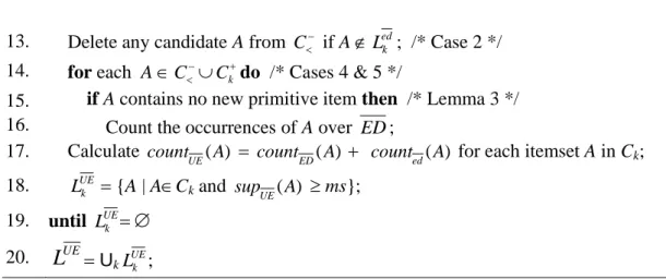
13. Delete any candidate A from C if A L ; /* Case 2 */edk 14. for each AC C do /* Cases 4 & 5 */k
15. if A contains no new primitive item then /* Lemma 3 */ 16. Count the occurrences of A over ED ;
17. Calculate count ( A)
UE countED( A) counted( A) for each itemset A in Ck; 18. LUEk {A | ACkand supUE( A) ms};
19. until UE k L 20.
L
UEUkLUEk ;Figure 9. Algorithm IDTE.
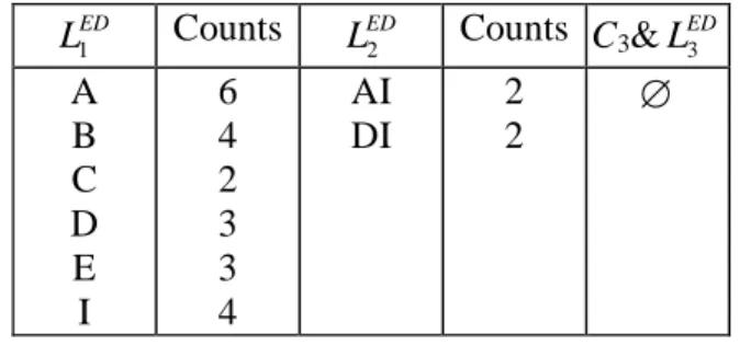
Consider the example in Figures 2 and 3. For simplicity, let item “A”stand for“PC”,“B”for“Desktop PC”,“C” for“Sony VAIO”,“D”for“IBM TP”,“E”for“Systemax V”,“F”for“PDA”,“G”for“MITAC Mio”,“H”for “ACER N”,“I”for“HP LaserJet”, “J”for “MC”, and “K”for “Gateway GE”.Theresulting item taxonomy is shown in Figure 10. Let ms20%. The set of frequent itemsets LED is shown in Table 3. The overall process of running this example using IDTE is illustrated in Figure 11.
Correctness: The correctness of algorithm IDTE lies mainly in two aspects: the procedure for candidate generation and that for inferring which candidate itemsets are frequent. The correctness of the former has been justified in [2]. For the latter, we need to verify that all cases dictated in Table 2. We only show the first case; the others can be proved in a similar way. Consider an unaffected candidate itemset A. From Lemma 3, countED(A) =
) ( A
countED . Since A is frequent in ED and ed , we have countED(A) |ED| ms and counted( A) | ed | ms.
Then countUE( A) = countED( A)+counted( A) (| ED | + | ed |) ms = |UE | ms. That is, supUE( A) ms and so A is frequent in UE .
3.2. Algorithm IDTE2
We now propose another algorithm called IDTE2. The main difference between IDTE and IDTE2 is in the approach for inferring whether or not an affected candidate itemset is frequent in the updated whole database, i.e., corresponding to Case 5 of Table 2. We observe that it is not always necessary to scan the whole database ED to know the occurrences of an affected candidate itemset and to determine if it is frequent in UE . Indeed, it suffices for the purpose if we know which part of the transactions is affected by the taxonomy evolution.
Original Extended Incremental Database (ed)
Updated Extended Incremental Database 9 10 B B TID Primitive Items Generalized Items K, I K, I 9 10 TID Primitive Items Generalized Items K, I K, I
Original Extended Database (ED)
1 6 5 4 3 2 A, B A TID Primitive Items Generalized Items A, B, F A, B A E C, E, G, H E D, I C, D D, I A, B 7 8 I I 1 6 5 4 3 2 B J TID Primitive Items Generalized Items B, F, J J J E C, E, G, H E D, I C, D D, I B 7 8 I I
Updated Extended Database
A E C I D B F H G I B E K H G J D F (ED) (ed)
Figure 10. Example of taxonomy evolution and incremental database.
Table 3. Summary for frequent itemsets and counts generated from ED. ED L1 Counts ED L2 Counts C3&LED3 A B C D E I 6 4 2 3 3 4 AI DI 2 2
Definition 3. A transaction is called an affected transaction if it contains at least one of the affected primitive items with respect to a taxonomy evolution.
Forexample,transactions1 and 2 areaffected transactionsin Figure12 becausethey contain affected items“G” and “E”.
Let and denote the part of affected transactions in ED and ED , respectively. Note that | ED | ED|, andED ED + . Then for a candidate itemset A, we have countED( A)countED( A)count( A) count( A) and countUE( A) countED( A) + counted( A). Therefore, if a candidate itemset A is an affected itemset and is frequent in ED, we only have to scanand to decide whether or not A is frequent in UE .
As for the affected candidate itemsets that are not frequent in ED, if A is frequent in ed , then we still have to scan ED to determine the occurrences of A in ED ; otherwise, let us consider the following lemma.
UnaffectedC2 AffectedC2 DE,EI BD,BI,BJ,DK, EJ,EK,IJ,IK,JK Load LED2 not inLED2 inLED2 DI Cal. support BI,DI,IJ,IK Generate UE L2 3 C Generate C3 Scan ED ) (C2 countED 0 0 1 BI BD BJ EJ 1 IJ 2 UE L2 Generate C2 BD,BI,BJ,DE,DI,DK,EI,EJ,EK,IJ,IK,JK 2 C ) (C2 counted DE 0 DI 0 DK 0 0 0 0 EJ EI EK IJ 0 IK 2 JK 0 BD 0 BI 2 BJ 0 Scan ed F, G, H B, D, E, F, G, H, I, J, K 1 C ) (C1 counted UnaffectedC1 Affected 1 C inLED1 not in LED1 Load LED1 D, E, I B, J, K Cal. support B, D, E, I, J, K Generate LUE1 UE L1 ) (C1 countED Scan ED E 0 D 0 B 2 K 2 J 0 I 2 H 0 G 0 F 0 Scan ed J 4 B 3
1 5 4 3 2 A, F A TID Primitive Items Generalized Items A, B F 1 5 4 3 2 D, G, H, I A, F D, E, I A, B TID Primitive Items Generalized Items H C, I I A, B F D, G, H, I D, E, I H C, I I
Original Extended Database(ED) Updated Extended Database A E C I D B F H G A E C I D B F H G ( ED )
Figure 12. Illustration of the concept of affected transactions.
Lemma 4. If an affected itemset A ED
L and count( A) count( A), then ALED. Proof. If A ED
L , then countED( A)|ED| ms. Note that |ED| | ED | and || ||. Hence countED( A) countED( A)+ (count( A)count( A))|ED| ms | ED |ms. Thus, ALED.
In light of Lemma 4, we scan the affected transactions inand , respectively, to count the occurrences of A. If the support count of A in is no larger than that in ,i.e., count( A) count( A), then A must be infrequent in ED and so can be pruned immediately; otherwise we have to scan ED to decide whether A is frequent or not.
Example 5. Consider Figure 12. Assume ms60% (3 transactions). Then items“B”and “F”are notfrequentin ED. That is, countED(B) and countED(F) are not available in L1ED . From and , we have
(B)
count count(F) 1, count(B) 0, count(F) 1, count(B) count(B) 1, and count(F) count(F)0. Items “B”and “F”are not frequent in ED according to Lemma 4. Therefore, there is no need to scan the transactions in ED to determine whether items “B”and “F”are frequent or not. This also reduces the number of candidates invoking the scanning of ED .
Table 4 summarizes the previous discussions and refines the cases for inferring frequent/infrequent itemsets and shows the corresponding actions. A further improvement for Case 7 is possible, as described below.
Lemma 5. If an itemset A contains at least one new generalized item, i.e., x A, x T T, then )
( A countED 0.
Proof. This is straightforward since a new generalized item only exists in , and so it does not appear in ED .
Table 4. Seven cases arising from the updated extended incremental database and the taxonomy evolution.
T T LED ed UE Action Case
frequent frequent no 1
infrequent undetermined compare sup ( A)
UE with ms 3
frequent undetermined scan ED 4
unaffected
infrequent infrequent no 2
frequent,
infrequent undetermined
scan& , cal. countED( A)
count( A)count( A)+counted( A) 5
frequent undetermined scan ED 6
affected
infrequent undetermined scan& , if count( A) count( A), then scan ED
7
The IDTE2 algorithm is described in Figure 13.
Input: (1) DB: original database; (2) db: incremental database; (3) ms: minimum support setting; (4) T: old item taxonomy; (5) T : new item taxonomy; (6) LED: set of original frequent itemsets.
Output:
L
UE: set of new frequent itemsets with respect to T and ed . Steps:1. Identify affected items;
2. Identify affected transactions,and ; 3. k1;
4. repeat
5. if kthen generate C1from T ; 6. elseCkapriori-gen(LUEk1);
7. Delete any candidate in Ckthat consists of an item and its ancestor;
8. Scan ed to count count ( A)
ed for each itemset A in Ck;
9. ed
k
L {A | ACkand suped( A)ms};
10. Load original frequent k-itemsets ED k L ;
11. Divide Ck into four subsets: C , C , Cand C ; /* Cand Cdenote affected itemsets in
ED k
L and not in ED k
L , respectively */
12. for each AC or A C do /* Cases 1, 3 & 5 */
14. Delete any candidate A from C if A L ; /* Case 2 */edk 15. Count the occurrences for each A in
C or C over ; /* Cases 5 & 7 */
16. Count the occurrences for each A in C , C or C over ; /* Cases 4, 5, 6 & 7 */ 17. for each AC do /* Case 5 */
18. Calculate countED( A)count( A)+count( A)+counted( A);
19. Delete any candidate A from C if A Ledk and count( A) count( A); /* Case 7 & Lemma 4 */ 20. for each AC do /* Case 4 */
21. if A contains no new primitive item then /* Lemma 3 */ 22. Count the occurrences of A over ED ;
23. for each AC do /* Case 6 & 7 */
24. if A contains no new item then /* Lemmas 3 & 5 */ 25. Count the occurrences of A over ED ;
26. Calculate countUE( A)countED( A)counted( A) for each ACkin Ck;
27. UE
k
L {A | ACkand supUE( A) ms};
28. until LUEk 29.
L
UEUkL ;UEkFigure 13. Algorithm IDTE2.
For illustration, let us consider Figure 10 and let ms 20% again. Transactions 1 to 6 in Figure 10 are affected transactions. The overall process of running this example using IDTE2 is illustrated in Figure 14.
Correctness: Note that IDTE2 differs from IDTE in the approach for inferring whether or not an affected candidate itemset is frequent afterwards. This corresponds to the Cases 5 and 7 in Table 4, whose correctness have been exposed in Lemmas 4 and 5.
3.3. Situation when obsolete transactions occur
In the aforementioned mining process, the proposed algorithms, IDTE and IDTE2, are based on the assumption of constant number of transactions, i.e., |ED|| ED |. However, some transactions may become null when all the items contained are obsolete and discarded. Under this circumstance, the frequent itemsets in ED remain frequent in ED , but the infrequent itemsets in ED may become frequent in ED because there are fewer transactions in
BD,BI,BJ,DE,DI,DK,EI,EJ,EK,IJ,IK,JK 2 C ) (C2 counted DE 0 DI 0 DK 0 0 0 0 EJ EI EK IJ 0 IK 2 JK 0 BD 0 BI 2 BJ 0 Scan ed ) (C1 count J 4 Cal. support Generate B 3 4 ScanED ScanED ) (C1 count Scan& UE L1 B, D, E, I, J, K UE L1 UnaffectedC1 in LED1 Load LED1 D, E, I F, G, H B AffectedC1 in LED1 not in LED1 not in LED1 K J B, D, E, F, G, H, I, J, K 1 C ) (C1 counted E 0 D 0 B 2 K 2 J 0 I 2 H 0 G 0 F 0 Scan ed GenerateC2
UnaffectedC2 Load LED2 AffectedC2
not inLED2 inLED2 DI not inLED2 inLED2 DE,EI BD,BI,BJ,DK, EJ,EK,IJ,IK,JK Cal. support BI,DI,IJ,IK Generate Generate C3 3 C ScanED ) (C2 count 0 0 BI BD EJ 1 IJ 2 ) (C2 count BJ 1 Scan& ScanED UE L2 UE L2
ED than in ED, i.e., |ED| | ED |. This implies that the scanning of ED is inevitable. Fortunately, not all such infrequent itemsets in ED have to be counted in ED . This can be clarified through the following lemmas.
Lemma 6. If an unaffected itemset A ED
L and counted( A)(| ed | (|ED| | ED |)) ms, then ALUE. Proof. We can derive
) ( A counted (| ed | (|ED| | ED |)) ms counted( A) + |ED|ms (| ed | + | ED |) ms counted( A) + countED( A) (| ed | + | ED |) ms counted( A) + countED( A) (| ed | + | ED |) ms countUE( A) |UE | ms.
For example, let |ED| 100, | ED | 100, | ed | 15, countED( A)39, counted( A)5 and ms 40%. We have )
( A
supUE countUE( A)/ |UE | ms 40%, and so A is infrequent in UE . Lemma 6 can verify this; counted( A) (| ed | (|ED| | ED |)) ms 5 (15 (100 100)) 40% 6. On the contrary, if | ED | 95, we have sup ( A)
UE 4411040%ms, and A is frequent in UE .
Therefore, during the course of counting a candidate itemset that satisfies Case 2, either running by algorithm IDTE or IDTE2, we can utilize Lemma 6 to decide whether to scan ED or not. More precisely, we just need to modify Step 13 in algorithm IDTE and 14 in IDTE2, as shown below; the other part remains unchanged.
Delete any candidate A from C if A Ledk and counted( A)(| ed | (|ED| | ED |)) ms; /* Case 2 & Lemma 6 */
Lemma 7. If an affected itemset A ED
L , count( A) count( A) and counted( A)(| ed | (|ED| | ED |)) ms, then AUE
L .
Proof. Analogous to Lemma 6, it is easy to derive )
( A
counted (| ed | (|ED| | ED |)) ms counted( A) + |ED|ms (| ed | + | ED |) ms
counted( A) + countED( A) (| ed | + | ED |) ms
counted( A) + countED( A)+ count( A)count( A) (| ed | + | ED |) ms counted( A) + countED( A) (| ed | + | ED |) ms
countUE( A) |UE | ms.
Lemma 7 indeed gives the evidence for avoiding a further scanning of ED to deal with Case 7 in algorithm IDTE2. It suffices for this purpose by revising Step 19 of algorithm IDTE2 as:
Delete any candidate A from C if A L ,edk count( A) count( A) and counted( A)(| ed | (|ED| | ED |)) ms; /* Case 7 & Lemma 7 */
4. Performance evaluation
In order to examine the performance of IDTE and IDTE2, we conducted experiments to compare their performance with that of applying generalized association mining algorithms, including Cumulate and Stratify, to the whole updated database. A synthetic dataset (denoted as Synth) generated by the IBM data generator [2]and a real dataset, Microsoft foodmart2000 (Foodmart for short), a supermarket data warehouse provided in MS SQL2000, are used in the experiments. The data for Foodmart is drawn from sales_fact_1997, sales_fact_1998 and sales_fact_dec_1998 in foodmart2000. The corresponding item taxonomy consists of three levels: There are 1560 primitive items in the first level (product), 110 generalized items in the second level (product_subcategory), and 47 generalized items in the top level (product_category).The parameter settings for both datasets are shown in Table 5. The comparisons are evaluated according to certain aspects: minimum support, incremental transaction size, and evolution degree. Here, the evolution degree is measured by the fraction of items that are affected. In the implementation of each algorithm, we also adopted two different support counting strategies: one with the horizontal counting [1][2][8][9] and the other with the vertical intersection counting [10][11]. For the horizontal counting, the algorithms are denoted as Cumulate(H), Stratify(H), IDTE(H) and IDTE2(H) while for the vertical intersection counting, the algorithms are denoted as Cumulate(V), Stratify(V), IDTE(V) and IDTE2(V). All experiments were performed on an Intel Pentium-IV 2.80GHz with 2GB RAM, running on Windows 2000. Note that in some figures, vertical scales are in logarithmic representation for better resolution. Minimum supports: We first compared the performance of these four algorithms with varying minimum supports at 40,000 incremental transactions for Synth and 5,000 incremental transactions for Foodmart with constant affected item percent 1.4% and 0.23%, respectively. The experimental results are shown in Figures 15
and 16 for Synth and Foodmart, respectively. It can be observed that with the same counting strategy, for Synth, IDTE(V) performs 110% and 388% faster than Cumulate(V) and Stratify(V) at ms0.5%, respectively, and for Foodmart, IDTE(V) performs 23% faster than Cumulate(V) and Stratify(V) at ms 0.05%. Among our algorithms, IDTE(V) and IDTE2(V) perform better than IDTE(H) and IDTE2(H).
Table 5. Default parameter settings for test datasets. Default value Parameter
Synth Foodmart |DB| Number of original transactions 177,783 35,000
|db| Number of incremental transactions 40,000 5,000 |t| Average size of transactions 16 12
N Number of items 231 1,717 R Number of groups 30 47 L Number of levels 3 3 F Fanout 5 14 10 100 1000 10000 0.5 1 1.5 2 2.5 3 ms % R u n ti m e (s ec .)
Cumulate(V) St rat ify(V) IDT E(V) IDT E2(V) Cumulate(H) St rat ify(H) IDT E(H) IDT E2(H)
log
Figure 15. Performance comparison of IDTE, IDTE2, Cumulate, and Stratify for different ms over Synth.
Transaction sizes: We then compared the four algorithms under varying transaction sizes at ms 1.0% with constant affected item percent 1.4% for Synth and at ms0.05% with affected item percent 0.23% for Foodmart. The other parameters are set to default values. Since Stratify presents poor performance at low ms for Foodmart, we only compare our algorithms with Cumulate. The results are depicted in Figures 17 and 18 for Synth and
Foodmart, respectively. It can be seen that all algorithms exhibit linear scalability. It is noteworthy that the horizontal version of our algorithms performs worse than the vertical version of Cumulate and Stratify for Synth, and the gap becomes more significant as the data size increases. This is because the processing time per transaction in the horizontal version of our algorithms is greater than that in the vertical versions of Cumulate and Stratify. 1 10 100 1000 10000 0.05 0.1 0.15 0.2 0.25 0.3 0.35 ms % R u n ti m e (s ec .) Cumulate(V) Stratify(V) IDT E(V) IDT E2(V) Cumulate(H) Stratify(H) IDT E(H) IDT E2(H)
log
Figure 16. Performance comparison of IDTE, IDTE2, Cumulate, and Stratify for different ms over Foodmart.
10 100 1000 10000
2 4 6 8 10 12 14 16
Number of incremental transctions (x 10,000)
R u n ti m e (s ec .)
Cumulat e(V) Strat ify(V) IDT E(V) IDT E2(V) Cumulat e(H) Strat ify(H) IDT E(H) IDT E2(H)
log
Figure 17. Performance comparison of IDTE, IDTE2, Cumulate, and Stratify for different transactions over Synth.
190 220 250 280 310 340 370 0.5 1 1.5 2 2.5 3
Number of incremental transctions (x 10,000)
R u n ti m e (s ec .)
Cumulate(V) IDT E(V) IDT E2(V) Cumulate(H) IDT E(H) IDT E2(H)
Figure 18. Performance comparison of IDTE, IDTE2, Cumulate, and Stratify for different transactions over Foodmart.
Evolution degree: Finally, we compared the four algorithms under varying degrees of evolution with ms1.0% and 40,000 incremental transactions for Synth and with ms 0.05% and 5,000 incremental transactions for Foodmart. The other parameters were set to default values. In the experiments, the affected generalizations are rearranged randomly, and the results are depicted in Figures 19 and 20 for Synth and Foodmart, respectively. As the results show, our algorithms are greatly affected by the degree of evolution, whereas Cumulate and Stratify exhibit steady performance. In both figures, IDTE(V) and IDTE2(V) exhibit better performance than IDTE(H) and IDTE2(H). In Figure 19, IDTE2(V) performs better than Cumulate(V) and Stratify(V) only under 3.5% of affected items while IDTE2(H) performs better than Cumulate(H) and Stratify(H) only under 4% of affected items. In Figure 20, IDTE2(H) performs better than Cumulate(H) only under 2.1% of affected items. We observe that IDTE2 takes longer process time than IDTE while increasing evolution degree since IDTE2 require processing both the original extended database ED and updated extended database ED simultaneously, and the advantage of Lemma 4 for IDTE2 disappears when the number of affected transactions increases.
In summary, we observe that IDTE(V) is superior to Cumulate(V) and Stratify(V), while IDTE(H) beats Cumulate(H) and Stratify(H) in all aspects of the evaluation. Moreover, all algorithms with vertical support counting strategy perform better than their counterparts with horizontal counting strategy.
10 100 1000 10000
0 3 6 9 12 15
Affected item percent %
R u n ti m e (s ec .)
Cumulate(V) St rat ify(V) IDT E(V) IDT E2(V) Cumulate(H) St rat ify(H) IDT E(H) IDT E2(H)
log
Figure 19. Performance comparison of IDTE, IDTE2, Cumulate, and Stratify for different degrees of evolution over Synth. 180 210 240 270 300 0 1 2 3 4 5 6
Affected item percent %
R u n ti m e (s ec .)
Cumulate(V) IDT E(V) IDT E2(V) Cumulate(H) IDT E(H) IDT E2(H)
Figure 20. Performance comparison of IDTE, IDTE2, Cumulate, and Stratify for different degrees of evolution over Foodmart.
5. Related Work
The problem of mining association rules in the presence of taxonomy information was initially addressed by Han et al. [3] and Srikant et al. [4], working independently. The problem was referred to as mining generalized association rules, aiming to find associations among items at any level of the taxonomy under the minimum support and minimum confidence constraints [4]. In Han et al., the problem mentioned was somewhat different from that considered in Srikant et al., because they generalized the uniform minimum support constraint to a form of assignment according to level, i.e., items at the same level received the same minimum support. The objective was to discover association level-by-level in a fixed hierarchy. That is, only associations among items on the same level were examined progressively from the top level to the bottom. Since then, several improvements or extensions have been proposed. Sriphaew and Theeramunkong [5] presented a method that exploits two types of constraints on generalized itemset relationships, called subset-superset and ancestor-descendant constraints, to speedup the mining process. In [6], Domingues and Rezende proposed an algorithm, called GART, which uses taxonomies, in the step of knowledge post-processing, to generalize and to prune uninteresting rules that may help the user to analyse the generated association rules.
The problem of updating association rules incrementally was first addressed by Cheung et al. [12]. They developed the essence of updating the discovered association rules when new transaction records are added to the database over time and proposed an algorithm called FUP (Fast UPdate). They further extended the model to incorporate the situations of deletion and modification [13]. Their approaches [12][13], however, did not consider the generalized items, and hence could not discover generalized association rules. Subsequently, a number of techniques have been proposed to improve the efficiency of incremental mining algorithms [14][15][16][17][18], although all of them were confined to mining associations among primitive items.
The maintenance issue for generalized association rules was also first studied by Cheung et al. [19], who proposed an extension of their FUP algorithm, called MLUp, to accomplish the task. In [20], Huang and Wu tackled the problem from a different point of view. Their approach used the original primitive frequent itemsets and association rules to directly generate new generalized association rules. Hong et al. [21] then considered the problem of updating generalized associations for record modification. They extended Han and Fu’sapproach[3] by introducing the concept of pre-large itemsets [14] to postpone the original database rescanning until a number of records have been modified. In [22], we have extended the problem of maintaining generalized associations incrementally to that incorporates non-uniform minimum support.
In summary, all previous work on mining generalized association rules required the taxonomy to be static, ignoring the fact that the taxonomy of items may change over time.
6. Conclusions
In this paper we have investigated the problem of updating generalized association rules when new transactions are inserted into the database and the taxonomy of items evolves over time. We also have presented two novel algorithms, IDTE and IDTE2, for updating generalized frequent itemsets. Empirical evaluation on synthetic data showed that the IDTE and IDTE2 algorithms are very efficient, significantly outperforming the contemporary generalized associations mining algorithms that are applied to the whole updated database.
In the future, we will extend the problem of updating generalized association rules to a more general model that adopts non-uniform minimum support to solve the problem that new introduced items usually have much lower supports. We will also apply the results to the problem of on-line discovery and maintenance of multi-dimensional association rules from a data warehouse data under evolution of taxonomy or attributes.
7. References
[1] R. Agrawal, T. Imielinski and A. Swami, Mining association rules between sets of items in large databases, Proceedings of 1993 ACM-SIGMOD International Conference on Management of Data (1993) 207-216. [2] R. Agrawal and R. Srikant, Fast algorithms for mining association rules, Proceedings of the 20th
International Conference on Very Large Data Bases (1994) 487-499.
[3] J. Han and Y. Fu, Discovery of multiple-level association rules from large databases, Proceedings of the 21st International Conference on Very Large Data Bases (1995) 420-431.
[4] R. Srikant and R. Agrawal, Mining generalized association rules, Proceedings of the 21st International Conference on Very Large Data Bases (1995) 407-419.
[5] K. Sriphaew and T. Theeramunkong, Fast algorithms for mining generalized frequent patterns of generalized association rules, IEICE Transaction on Information and Systems 87(3) (2004) 761-770.
[6] M.A. Domingues and S.O. Rezende, Using taxonomies to facilitate the analysis of the association rules, Proceedings of the Second International Workshop on Knowledge Discovery and Ontologies (2005) 59-66. [7] J. Han and Y. Fu, Dynamic generation and refinement of concept hierarchies for knowledge discovery in
databases, Proceedings of AAAI’94 Workshop on Knowledge Discovery in Databases (1994) 157-168. [8] S. Brin, R. Motwani, J.D. Ullman and S. Tsur, Dynamic itemset counting and implication rules for
market-basket data, SIGMOD Record (26) (1997) 255-264.
[9] J.S. Park, M.S. Chen and P.S. Yu, An effective hash-based algorithm for mining association rules, Proceedings of ACM-SIGMOD International Conference on Management of Data (1995) 175-186.
[10] A. Savasere, E. Omiecinski and S. Navathe, An efficient algorithm for mining association rules in large databases, Proceedings of the 21st International Conference on Very Large Data Bases (1995) 432-444. [11] M.J. Zaki, Scalable algorithms for association mining, IEEE Transactions on Knowledge and Data
Engineering 12(2) (2000) 372-390.
[12] D.W. Cheung, J. Han, V.T. Ng and C.Y. Wong, Maintenance of discovered association rules in large databases: An incremental update technique, Proceedings of 1996 International Conference on Data Engineering (1996) 106-114.
[13] D.W. Cheung, S.D. Lee and B. Kao, A general incremental technique for maintaining discovered association rules, Proceedings of DASFAA'97 (1997) 185-194.
[14] T.P. Hong, C.Y. Wang and Y.H. Tao, A new incremental data mining algorithm using pre-large itemsets, Intelligent Data Analysis 5(2) (2001) 111-129.
[15] K.K. Ng and W. Lam, Updating of association rules dynamically, Proceedings of 1999 International Symposium Database Applications in Non-Traditional Environments (2000) 84-91.
[16] N.L. Sarda and N.V. Srinivas, An adaptive algorithm for incremental mining of association rules, Proceedings of the 9th International Workshop on Database and Expert Systems Applications (1998) 240-245.
[17] S. Thomas, S. Bodagala, K. Alsabti and S. Ranka, An efficient algorithm for the incremental updation of association rules in large databases, Proceedings of the 3rd International Conference on Knowledge Discovery and Data Mining (1997) 263-266.
[18] A. Veloso, W. Meira Jr., M. Carvalho, S. Parthasarathy and M.J. Zaki, Parallel, incremental and interactive mining for frequent itemsets in evolving databases, Proceedings of the 6th International Workshop on High Performance Data Mining: Pervasive and Data Stream Mining (2003).
[19] D.W. Cheung, V.T. Ng and B.W. Tam, Maintenance of discovered knowledge: a case in multi-level association rules, Proceedings of 1996 International Conference on Knowledge Discovery and Data Mining (1996) 307-310.
[20] Y.F. Huang and C.M. Wu, Mining generalized association rules using pruning techniques, Proceedings of 2002 IEEE International Conference on Data Mining (2002) 227-234.
[21] T.P. Hong, T.J. Huang and C.S. Chang, Maintenance of multiple-level association rules for record modification, Proceedings of 2004 IEEE International Conference on Systems, Man & Cybernetics (2004) 3140-3145.
[22] M.C. Tseng and W.Y. Lin, Maintenance of generalized association rules with multiple minimum supports, Intelligent Data Analysis 8(4) (2004) 417-436