IEEE 802.16m 之初始下行同步

國

立

交

通

大

學

電機學院通訊與網路科技產業研發碩士班

碩

士

論

文

IEEE 802.16m 之初始下行同步

Initial Downlink Synchronization for IEEE 802.16m

研

究

生：陸凱暐

指導教授：林大衛 博士

張文鐘 博士

IEEE 802.16m 之初始下行同步

Initial Downlink Synchronization for IEEE 802.16m

研 究

生：陸凱暐

Student：Kai-Wei Lu

指導教授：林大衛 Advisor：Dr. David W. Lin

國 立 交 通 大 學

電機學院通訊與網路科技產業研發碩士班

碩 士 論 文

A Thesis

Submitted to College of Electrical and Computer Engineering National Chiao Tung University

in partial Fulfillment of the Requirements for the Degree of

Master in

Industrial Technology R & D Master Program on Communication Engineering

February 2010

Hsinchu, Taiwan, Republic of China

IEEE 802.16m 之初始下行同步

學生：陸凱暐

指導教授

：

林大衛 博士

張文鐘 博士

國立交通大學電機學院產業研發碩士班

摘

要

當一個行動電話開始要進入網路的時候，我們必須與基地台做初始的同步。在初始的同步 中，包含了符元時間偏移、載波偏移和前置符元序號(preamble index)需要同步估測。我們利用 前置符元的功率較一般資料符元(data symbol)大的特性做功率移動累加，藉由找到累加結果的 峰值來估測前置符元的起始位置。由此起始位置向後推算一個符元長度以當作我們所估測出來 的前置符元，而與真實的前置符元存在一個相位性錯誤(phase error)。我們利用此估測出來的 前置符元推導其近似最大可能性估測(quasi maximum likelihood)以求得小數部分載波偏移和導 出前置符元的通道估測的式子。我們在頻域上將此通道估測的式子經由估測出來的小數部分載 波偏移補償之後，代入由合理範圍的整數部分載波偏移和不同的前置符元而得到的通道脈衝響 應。再計算這些通道脈衝響應不同的精準符碼時間偏移序號 64 點功率和並且選出最大的那一 個，其所在的整數部分載波偏移、前置符元和精準符碼時間偏移序號即為此聯合估測的結果。 本篇論文介紹 IEEE 802.16m 系統裡關於下行初始同步的問題、演算法推導、以及程式模 擬方面的議題。首先簡介 IEEE 802.16m 下行的標準機制及相關架構，接著提出同步問題並提 供演算法的設計發想及推導，而後將整個演算法的流程用浮點數運算來驗證，設計出一個合理 的 IEEE 802.16m 接收訊號模型，在可加性白色高斯雜訊(additive white Gaussian noise, AWGN) 通道之下得到的數據來驗證演算法的特性，然後在多路徑衰減(multipath fading)通道傳輸中使 用數種不同多路徑通道、相對移動車速以及訊雜比(signal to noise ratio, SNR)來測試演算法對多

Initial Downlink Synchronization for IEEE 802.16m

Student: Kai-Wei Lu

Advisor:

Dr. David W. Lin

Dr. Wen-Thong Chang

Industrial Technology R & D Master Program of

Electrical and Computer Engineering College

National Chiao Tung University

ABSTRACT

This thesis introduces some topics about initial downlink synchronization, algorithm derivations, and program simulations of IEEE 802.16m system.

When a mobile station entering to the network, it needs to perform initial synchronization, including of symbol timing offset, carrier frequency offset and preamble index. We utilize the trait which the power of preamble is larger than it of the common data symbol to compute the moving power sum, and then estimate the left boundary of preamble by finding out the peak value of moving power sum. A symbol period from this estimated boundary is regarded as the estimated preamble, which has a phase noise with the exact preamble. We derive the quasi maximum likelihood estimation from the likelihood function of the estimated preamble to obtain fractional carrier frequency offset (FCFO) and the formula of channel estimation. After compensating the estimated fractional carrier frequency offset to the formula of channel estimation, we substitute several reasonable integral carrier frequency offsets (ICFOs) and primary advanced preambles (PA-Preambles) into this formula and obtain channel impulse responses (CIRs). After that, we compute different fine timing offset index 64-points power sum of these CIRs and find out the peak value whose ICFO, PA-Preamble index, and fine timing offset index are regarded as the result of the joint estimation.

In terms of simulations, above all, we present a reasonable received signal model of IEEE 802.16m, and then simulate our algorithm in floating point under AWGN (additive white Gaussian noise) channel to verify its performance. Moreover, we test this algorithm under different multipath fading channels, Pedestrian B and SUI-5, at different speed which cause Doppler shifts, and signal to noise ratio (SNR) to observe the effect on this algorithm.

誌謝

這篇論文能夠順利完成，首先要感謝的人是我的指導教授林大衛老師以及張 文鐘老師。在兩年半的研究所生涯當中，由於老師的細心指導及在專業領域的博 學精深，令我在研究的精神與方法上獲益良多且終身受用。 此外，感謝通訊電子與訊號處理實驗室所有的成員，包含各位師長、同學、 學長姐與學弟妹們。感謝洪崑健學長、林鴻志學長、吳俊榮學長、王柏森學長以 及王海薇學姐給予我在研究過程上的指導與建議，還有劭學、志偉、豐進、世榮、 清德、振偉、重佑和藹璇等同學，因為能和你們共同討論、分享求學的經驗及一 路上的相互扶持，讓這兩年半的研究生涯充滿歡樂與回憶。 最後，我要感謝我的家人們以及女友，感謝他們一直都在背後支持我，在求 學過程中總是不斷的鼓勵、體諒及包容，是我精神與實質上最大的支柱，沒有他 們無保留的給予，一切的美好與榮耀將不復存在。 在此，虔誠的將此篇論文獻給所有陪伴著我走過這一段歲月的每一個人。 陸凱暐 民國九十九年二月 於風城 ･ 新竹

Contents

1 Introduction 1

2 Overview of the IEEE 802.16m Standard 3

2.1 Overview of OFDMA [1], [2] . . . 3

2.1.1 Cyclic Prefix . . . 4

2.1.2 Discrete-Time Baseband Equivalent System Model . . . 5

2.2 Basic OFDMA Symbol Structure in IEEE 802.16m [3] . . . 6

2.2.1 OFDMA Basic Terms . . . 7

2.2.2 Frequency Domain Description . . . 8

2.2.3 Primitive Parameters . . . 8

2.2.4 Derived Parameters . . . 8

2.2.5 Frame Structure . . . 9

2.3 Downlink Transmission in IEEE 802.16m [3] . . . 11

2.3.1 Subband Partitioning . . . 12

2.3.2 Miniband Permutation . . . 13

2.3.3 Frequency Partitioning . . . 15

2.4 Cell-Specific Resource Mapping [3] . . . 19

2.4.1 CRU/DRU Allocation . . . 19

2.4.2 Subcarrier Permutation . . . 20

2.4.3 Random Sequence Generation . . . 22

2.5 Advanced Preamble Structure (A-Preamble) [3] . . . 22

2.5.1 Primary Advanced Preamble (PA-Preamble) . . . 23

3 Initial Downlink Synchronization 28

3.1 The Initial Synchronization Problem . . . 28

3.2 Derivation of the Initial Synchronization Procedure . . . 29

3.2.1 Coarse Timing Synchronization . . . 30

3.2.2 Estimation of Fractional Carrier Frequency Offset . . . 32

3.2.3 Jointly Integral CFO, PA-Preamble Index, Channel Estimation and Fine Timing Offset Searching . . . 40

3.2.4 Overall Block Diagram . . . 41

3.3 Identification of the SA-Preamble . . . 41

4 Simulation Study 45 4.1 System Parameters and Channel Environments . . . 45

4.1.1 System Parameters . . . 45

4.1.2 Power Delay Profiles . . . 45

4.2 Simulation Results . . . 47

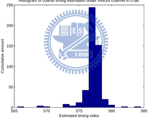
4.2.1 Coarse Timing Estimation . . . 47

4.2.2 Fractional CFO . . . 49

4.2.3 Joint Estimation of Integral CFO, PA-Preamble Index, Channel Response and Fine Timing . . . 50

4.2.4 Overall Timing Estimation . . . 52

5 Conclusion and Future Work 69 5.1 Conclusion . . . 69

List of Figures

2.1 Discrete-time model of the baseband OFDMA system (from [1]). . . 4 2.2 OFDMA symbol time structure (Fig. 428 in [3]). . . 5 2.3 Discrete-time baseband equivalent of an OFDMA system with M users

(from [2]). . . 6 2.4 OFDMA parameters (Table 647 in [3]). . . 9 2.5 More OFDMA parameters (Table 647 in [3]). . . 10 2.6 Basic frame structure for 5, 10 and 20 MHz channel bandwidths (Fig. 430

in [3]). . . 10 2.7 Example of downlink physical structure (Fig. 449 in [3]). . . 12 2.8 Mapping between SAC and KS Bfor 10 or 20 MHz band (Table 649 in [3]). 14

2.9 Mapping between SAC and KS Bfor 5 MHz band (Table 650 in [3]). . . . 14

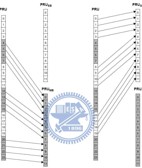
2.10 PRU to PRUS Band PRUMB mapping for BW = 5 MHz, and KS B=3 (Fig.

450 in [3]). . . 15 2.11 Mapping from PRUs to PRUS Band PPRUMB for BW = 5 MHz and KS B

= 3 (Fig. 451 in [3]). . . 16 2.12 Mapping between DFPC and frequency partitioning for 10 or 20 MHz

band (Table 651 in [3]). . . 17 2.13 Mapping between DFPC and frequency partitioning for 5 MHz band

(Ta-ble 652 in [3]). . . 17 2.14 Frequency partitioning for BW = 5 MHz, KS B= 3, FPCT = 2, FPS = 12,

and FPSC = 1 (Fig. 452 in [3]). . . 18 2.15 Location of the A-Preamble symbol (re-arranged from Fig. 500 in [3]). . . 23 2.16 PA-Preamble symbol structure of 5-MHz system (Fig. 501 in [3]). . . 24

2.17 PA-Preamble symbol structure of 10 MHz system. . . 24

2.18 PA-Preamble symbol structure of 20 MHz system. . . 24

2.19 PA-Preamble Series (Table 780 in [3]). . . 25

2.20 SA-Preamble symbol structure of 5 MHz. . . 26

2.21 The allocation of sequence block for each FFT size (Fig. 503 in [3]). . . . 27

2.22 SA-Preamble symbol structure for 512-FFT (Fig. 504 in [3]). . . 27

3.1 Window sliding structure. . . 29

3.2 576 points power sum under AWGN in 0 dB. . . 31

3.3 576 points power sum under AWGN in 10 dB. . . 32

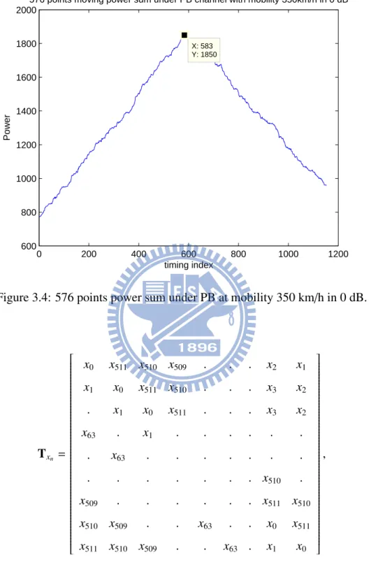
3.4 576 points power sum under PB at mobility 350 km/h in 0 dB. . . 33

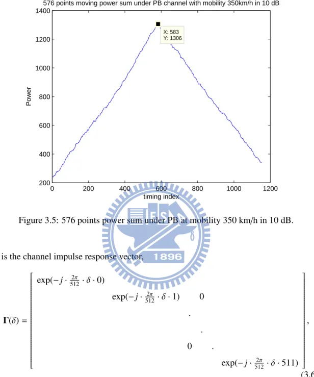
3.5 576 points power sum under PB at mobility 350 km/h in 10 dB. . . 34

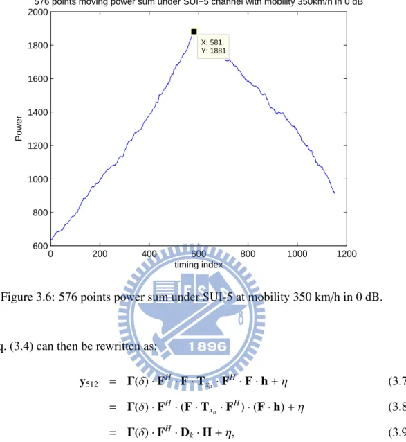
3.6 576 points power sum under SUI-5 at mobility 350 km/h in 0 dB. . . 35

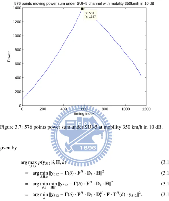
3.7 576 points power sum under SUI-5 at mobility 350 km/h in 10 dB. . . 36

3.8 Channel impulse response of PB channel. . . 37

3.9 Channel impulse response of SUI-5 channel. . . 38

3.10 The estimated CIR with accurate ICFO, 8, compensating and correct PA-Preamble index, 1, under PB channel with 120 km/h, 0dB in SNR. . . 41

3.11 The CIR with the inaccurate ICFO, 6, compensating and incorrect PA-Preamble index, 0, under PB channel with 120 km/h, 0dB in SNR. . . 42

3.12 Block diagram of initial DL synchronization. . . 43

4.1 Histogram of coarse timing estimation under AWGN channel in 0 dB. . . 49

4.2 Histogram of coarse timing estimation under AWGN channel in 10 dB. . 50

4.3 Histogram of coarse timing estimation under PB at 3 km/h in 0 dB. . . 51

4.4 Histogram of coarse timing estimation under PB at 3 km/h in 10 dB. . . . 52

4.5 Histogram of coarse timing estimation under PB at 120 km/h in 0 dB. . . 53

4.6 Histogram of coarse timing estimation under PB at 120 km/h in 10 dB. . . 54

4.7 Histogram of coarse timing estimation under SUI-5 at 3 km/h in 0 dB. . . 54

4.8 Histogram of coarse timing estimation under SUI-5 at 3 km/h in 10 dB. . 55

4.10 Histogram of coarse timing estimation under SUI-5 at 120 km/h in 10 dB. 56 4.11 Simulation results of FCFO estimation under PB, SUI5 and AWGN channel. 57

4.12 Histogram of fine timing estimation under AWGN channel in 0 dB. . . 58

4.13 Histogram of fine timing estimation under AWGN channel in 10 dB. . . . 58

4.14 Histogram of fine timing estimation under PB at 3 km/h in 0 dB. . . 59

4.15 Histogram of fine timing estimation under PB at 3 km/h in 10 dB. . . 59

4.16 Histogram of fine timing estimation under PB at 120 km/h in 0 dB. . . 60

4.17 Histogram of fine timing estimation under PB at 120 km/h in 10 dB. . . . 60

4.18 Histogram of fine timing estimation under SUI-5 at 3 km/h in 0 dB. . . . 61

4.19 Histogram of fine timing estimation under SUI-5 at 3 km/h in 10 dB. . . . 61

4.20 Histogram of fine timing estimation under SUI-5 at 120 km/h in 0 dB. . . 62

4.21 Histogram of fine timing estimation under SUI-5 at 120 km/h in 10 dB. . 62

4.22 Histogram of ICFO estimation under SUI-5 at 120 km/h in 0 dB. . . 63

4.23 Histogram of PID estimation under SUI-5 at 120 km/h in 0 dB. . . 63

4.24 Histogram of timing estimation under AWGN in 0 dB. . . 64

4.25 Histogram of timing estimation under AWGN in 10 dB. . . 64

4.26 Histogram of timing estimation under PB at 3 km/h in 0 dB. . . 65

4.27 Histogram of timing estimation under PB at 3 km/h in 10 dB. . . 65

4.28 Histogram of timing estimation under PB at 120 km/h in 0 dB. . . 66

4.29 Histogram of timing estimation under PB at 120 km/h in 10 dB. . . 66

4.30 Histogram of timing estimation under SUI-5 at 3 km/h in 0 dB. . . 67

4.31 Histogram of timing estimation under SUI-5 at 3 km/h in 10 dB. . . 67

4.32 Histogram of timing estimation under SUI-5 at 120 km/h in 0 dB. . . 68

List of Tables

2.1 PRU Structure for Different Types of Subframes . . . 7

4.1 System Parameters Used in Our Study . . . 46

4.2 SUI-1 Channel Model . . . 46

4.3 SUI-2 Channel Model . . . 46

4.4 SUI-3 Channel Model . . . 47

4.5 SUI-4 Channel Model . . . 47

4.6 SUI-5 Channel Model . . . 47

4.7 SUI-6 Channel Model . . . 48

4.8 ETSI “Vehicular A” Channel Model [8] . . . 48

4.9 Pedestrain B (PB) Channel Model . . . 49

Chapter 1

Introduction

ITU-R defined the criterion of the fourth-generation (4G) mobile communication standard IMT-Advanced formally in June 2003, that the data rate need be higher than 100 Mbps in the environment with the high mobility and 1 Gbps in the static environ-ment. Therefore, IEEE 802.16m Task Group (TGm) has set up the 802.16m (i.e., Ad-vanced WiMAX or WiMAX 2) since December 2006 in order to compete for the fourth-generation standard. The new frame structure developed by IEEE 802.16m is such that it can be compatible with IEEE 802.16e, reduce communication latency, support relay and coexist with other radio access techniques, so that it can become one of the promising candidates of 4G.

In this thesis, we consider the IEEE 802.16m system in time-division duplex (TDD) mode, where downlink (DL) and uplink (UL) transmissions are time multiplexed in each frame. Our study focuses on the techniques of downlink initial synchronization, includ-ing problem formulation, algorithm derivation and computer simulation. In this, we uti-lize the special structure of the primary advanced preamble (PA-Preamble) defined in the draft IEEE 802.16m standard. The synchronization work involves frequency recovery, timing recovery and bandwidth detection, where bandwidth detection is accomplished by identifying the PA-Preamble index. In the procedure that we have developed, channel estimation is also obtained simultaneously.

The contributions of this work are as follows:

timing by the difference of power between the PA-Preamble and other data symbols. • In order to estimate fractional carrier frequency offset (FCFO), we derive a sim-plified maximum likelihood estimation and get a result which is the same with the Moose algorithm.

• From the process of FCFO estimation, we can get the least-square estimation of channel impulse response of the PA-Preamble and utilize its characteristic of power centralization to search integral carrier frequency offset (ICFO), preamble index (PID) and the fine timing offset jointly.

This thesis is organized as follows. We will first introduce the IEEE 802.16m standard briefly in chapter 2. We will analyze the synchronization problems and present the overall procedure in chapter 3. Chapter 4 will discuss the simulation results under the different environments. Finally, the conclusion will be given in chapter 5, where we will also point out some potential future work.

Chapter 2

Overview of the IEEE 802.16m

Standard

The IEEE 802.16m standard is based on orthogonal frequency division multiplex-ing (OFDM) and orthogonal frequency division multiple access (OFDMA). The IEEE 802.16m Task Group intends to complete the first version of the standard in 2010. In this chapter, we first introduce some basic concepts regarding OFDM and OFDMA. Then we give an overview of the draft IEEE 802.16m standard. For the sake of simplicity, we only introduce the specifications that are most relevant to our study.

2.1 Overview of OFDMA [1], [2]

OFDMA is considered one most appropriate scheme for future wireless systems, including 4G broadband wireless networks. In a typical OFDMA system, users simulta-neously transmit their data by modulating mutually exclusive sets of orthogonal subcar-riers, so that each user’s signal can be separated in the frequency domain. One typical structure is subband OFDMA, where all available subcarriers are divided into a number of subbands and each user is allowed to use one or more subbands for the data transmis-sion. Usually, pilot symbols are employed for the estimation of channel state information (CSI) within the subband. IEEE 802.16e and 802.16m are examples of such systems. Figure 2.1 shows an OFDMA system in which active users simultaneously communicate

with the base station (BS).

2.1.1 Cyclic Prefix

Cyclic prefix (CP) or guard time is used in OFDM and OFDMA systems to overcome the intersymbol and interchannel intercarrier problems. The multiuser channel is usually assumed to be substantially invariant within one-block (or one-symbol) duration. The channel delay spread plus symbol timing mismatch is usually assumed to be smaller than the CP duration. In this condition, users do not interfere with each other in the frequency domain when their signal are properly synchronized in frequency and in time.

A CP is a copy of the last part of the OFDMA symbol (see Fig. 2.2). A copy of the last Tg of the useful symbol period is used to collect multipaths while maintaining the

orthogonality of subcarriers. However, the transmitter energy increases with the length of the guard time while the receiver energy remains the same (the CP is discarded in the receiver). So there is a 10 log(1 − Tg/(Tb+ Tg))/log(10) dB loss in Eb/N0.

Figure 2.2: OFDMA symbol time structure (Fig. 428 in [3]).

2.1.2 Discrete-Time Baseband Equivalent System Model

The material in this subsection is mainly taken from [2]. Consider an OFDMA system with M active users sharing a bandwidth of B =1

T Hz (T is the sampling period) as

shown in Fig. 2.3. The system consists of K subcarriers of which Kuare useful subcarriers

(excluding guard bands and DC subcarrier). The users are allocated non-overlapping subcarriers according to their needs.

Let the discrete-time baseband channel consists of L multipath components as

h(l) =

L−1

X

m=0

hmδ(l − lm), (2.1)

where hm is a zero-mean complex Gaussian random variable with E[hih∗_j] = 0 for i , j.

In the frequency domain,

H = Fh, (2.2)

where H = [H0, H1, ..., HK−1]T, h = [h0, ..., hL−1, 0, ..., 0]T and F is K-point discrete fourier

transform (DFT) matrix. The impulse response length lL−1is upper bounded by the length

of CP (Lcp).

The received signal in the frequency domain is given by Yn =

M

X

i=1

Xi,nHi,n+ Vn, (2.3)

where Xi,n = diag(Xi,n,0, ..., Xi,n,K−1) is K × K diagonal data matrix and Hi,n is the K × 1

channel vector (2.2) corresponding to the ith user in the nth symbol. The noise vector Vn

is distributed as CN(0, σ2_I

Figure 2.3: Discrete-time baseband equivalent of an OFDMA system with M users (from [2]).

2.2 Basic OFDMA Symbol Structure in IEEE 802.16m

[3]

The Advanced Air Interface defined by IEEE 802.16m is designed for nonline-of-sight (NLOS) operation in the licensed frequency bands below 6 GHz. The Advanced Air Interface supports time-division-duplexing (TDD) and frequency-division-duplexing (FDD) duplex modes, including half FDD (H-FDD) mobile station (MS) operation. Un-less otherwise specified, the frame structure attributes and baseband processing are com-mon for all duplex modes.

The Advanced Air Interface uses OFDMA as the multiple access scheme in the down-link and updown-link. The material of this section is mainly taken from [3].

2.2.1 OFDMA Basic Terms

We introduce some basic terms in the OFDMA physical layer (PHY) of IEEE 802.16m. These definitions help us understand the concepts of subcarrier allocation and transmis-sion in IEEE 802.16m.

• Physical and logical resource units: A physical resource unit (PRU) is the basic physical unit for resource allocation. It comprises Psc consecutive subcarriers by

Nsym consecutive OFDMA symbols, where Psc = 18 and Nsym = 6 for type-1

subframes, Nsym = 7 for type-2 subframes, and Nsym = 5 for type-3 subframes.

Table. 2.2.1 illustrates the PRU’s sizes for different subframe types. A logical re-source unit (LRU) is the basic logical unit for distributed and localized rere-source allocations. An LRU is Psc· Nsym subcarriers for type-1, type-2, and type-3

sub-frames. The LRU includes the pilots that are used in a PRU. The effective number of data subcarriers in an LRU depends on the number of allocated pilots.

• Distributed resource unit: A distributed resource unit (DRU) contains a group of subcarriers which are spread across the distributed resource allocations within a frequency partition. The size of DRU equals the size of PRU, i.e., Psc subcarriers

by NsymOFDMA symbols.

• Contiguous resource unit: The localized resource unit, also known as contiguous resource unit (CRU), contains a group of subcarriers which are contiguous across the localized resource allocations. The size of CRU equals the size of PRU, i.e., Psc

subcarriers by NsymOFDMA symbols.

Table 2.1: PRU Structure for Different Types of Subframes Subframe Type Number of Subcarriers Number of Symbols

1 18 6

2 18 7

2.2.2 Frequency Domain Description

The frequency domain description includes the basic structure of an OFDMA sym-bol. An OFDMA symbol is made up of subcarriers, the number of which determines the DFT size used. There are several subcarrier types:

• Data subcarriers: for data transmission.

• Pilot subcarriers: for various estimation purposes.

• Null subcarriers: no transmission at all, for guard bands and DC subcarrier. The purpose of the guard bands is to help enable proper bandlimiting.

2.2.3 Primitive Parameters

Four primitive parameters characterize the OFDMA symbols: • BW: the nominal channel bandwidth.

• Nused: number of used subcarriers (which includes the DC subcarrier).

• n: sampling factor. This parameter, in conjunction with BW and Nused, determines

the subcarrier spacing and the useful symbol time. This value is given in Figs. 2.4 and 2.5 for each nominal bandwidth.

• G: This is the ratio of CP time to “useful” time, i.e., Tcp/Ts. The following values

are supported: 1/16, 1/8, and 1/4.

2.2.4 Derived Parameters

The following parameters are defined in terms of the primitive parameters. • NFFT: smallest power of two greater than Nused.

• Useful symbol time: Tb = 1/4 f .

• CP time: Tg = G × Tb.

• OFDMA symbol time: Ts= Tb+ Tg.

• Sampling time: Tb/NFFT.

2.2.5 Frame Structure

The advanced air interface basic frame structure is illustrated in Fig. 2.6. Each 20-ms superframe is divided into four 5-20-ms radio frames. When using the same OFDMA parameters as in Figs. 2.4 and 2.5 with channel bandwidth of 5, 10, or 20 MHz, each

Figure 2.5: More OFDMA parameters (Table 647 in [3]).

Figure 2.6: Basic frame structure for 5, 10 and 20 MHz channel bandwidths (Fig. 430 in [3]).

5-ms radio frame further consists of eight subframes, for G = 1/8 and 1/16. With channel bandwidth of 8.75 or 7 MHz, each 5-ms radio frame further consists of seven and six subframes, respectively for G = 1/8 and 1/16. In the case of G = 1/4, the number

of subframes per frame is one less than that of other CP lengths for each bandwidth case. A subframe forms the unit of assignment for either downlink (DL) or uplink (UL) transmission. There are four types of subframes:

• Type-1 subframe consists of six OFDMA symbols. • Type-2 subframe consists of seven OFDMA symbols. • Type-3 subframe consists of five OFDMA symbols.

• Type-4 subframe consists of nine OFDMA symbols. This type shall be applied only to UL subframe for the 8.75 MHz channel bandwidth when supporting the WirelessMAN-OFDMA frames.

The basic frame structure is applied to FDD and TDD duplexing schemes, including H-FDD MS operation. The number of switching points in each radio frame in TDD systems shall be two, where a switching point is defined as a change of directionality, i.e., from DL to UL or from UL to DL.

A data burst shall occupy either one subframe (i.e., the default transmission time in-terval [TTI] transmission) or contiguous multiple subframes (i.e., the long TTI transmis-sion). The long TTI in FDD shall be 4 subframes for both DL and UL. The long TTI in TDD shall be the whole DL (UL) subframes for DL (UL) in a frame. Every super-frame shall contain a supersuper-frame header (SFH). The SFH shall be located in the first DL subframe of the superframe and shall include broadcast channels.

2.3 Downlink Transmission in IEEE 802.16m [3]

Again, this section is mainly taken from [3]. Each DL subframe is divided into 4 or fewer frequency partitions, each partition consisting of a set of physical resource units across the total number of OFDMA symbols available in the subframe. Each frequency partition can include contiguous (localized) and/or non-contiguous (distributed) physical resource units (PRUs). Each frequency partition can be used for different purposes such as fractional frequency reuse (FFR) or multicast and broadcast services (MBS). Fig. 2.7

illustrates the downlink physical structure in an example of two frequency partitions with frequency partition 2 including both contiguous and distributed resource allocations.

2.3.1 Subband Partitioning

The PRUs are first subdivided into subbands and minibands where a subband com-prises N1 adjacent PRUs and a miniband comprises N2 adjacent PRUs, where N1 = 4

and N2 = 1. Subbands are suitable for frequency selective allocations as they provide a

contiguous allocation of PRUs in frequency. Minibands are suitable for frequency diverse allocation and are permuted in frequency.

The number of subbands reserved is denoted by KS B. The number of PRUs allocated

to subbands is denoted by LS B, where LS B = N1· KS B, depending on system bandwidth.

A 4 or 3-bit field called Subband Allocation Count (SAC) determines the value of KS B.

The remainder of the PRUs are allocated to minibands. The number of minibands in an allocation is denoted by KMB. The number of PRUs allocated to minibands is denoted

by LMB, where LMB = N2 · KMB. The total number of PRUs is denoted NPRU where

NPRU = LS B+ LMB. The maximum number of subbands that can be formed is denoted

Nsubwhere Nsub= NPRU/N1.

Figs. 2.8 and 2.9 show the mapping between SAC and KS B for the 10 and 20 MHz

bands and the 5 MHz band, respectively.

PRUs are partitioned and reordered into two groups called subband PRUs and mini-band PRUs and denoted PRUS B and PRUMB, respectively. The set PRUS Bis numbered

from 0 to LS B−1,and the set PRUMBis numbered from 0 to LMB−1. Equation (2.4) defines

the mapping of PRUs to PRUS B, and (2.6) the mapping of PRUs to PRUMB. Fig. 2.10

il-lustrates the PRU to PRUS Band PRUMBmappings for a 5 MHz bandwidth with KS Bequal

to 3. PRUS B[ j] = PRU[i], j = 0, 1, ..., LS B− 1, (2.4) where i = N1· {{d Nsub KS B e · b j N1 c + bb j N1 c · GCD(Nsub, d Nsub KS Be) Nsub c} mod Nsub} + j · N1 (2.5)

with GCD(x, y) being the greatest common divisor of x and y.

PRUMB[k] = PRU[i], k = 0, 1, ..., LMB− 1, (2.6) where i =                    N1· {dN_Ksub_{S B}·e · bk+L_N1S Bc + bbk+L_N1S Bc · GCD(Nsub,dNsub_{KS B}e)

Nsub c} mod Nsub

+(k + LS B) mod N1, KS B > 0,

i = k, KS B = 0.

(2.7)

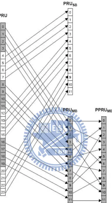
2.3.2 Miniband Permutation

The miniband permutation maps the PRUMBs to Permuted PRUMBs (PPRUMBs) to

ensure that frequency diverse PRUs are allocated to each frequency partition. Fig. 2.11 shows an example. The following gives the mapping between PRUMB and PPRUMB:

PRUMB[ j] = PRU[i], j = 0, 1, ..., LMB− 1, (2.8)

where

i = (q( j) mod D) · P + bq( j)

Figure 2.8: Mapping between SAC and KS Bfor 10 or 20 MHz band (Table 649 in [3]).

Figure 2.9: Mapping between SAC and KS Bfor 5 MHz band (Table 650 in [3]).

P = min(KMB, N1/N2), (2.10) r( j) = max( j − ((KMB mod P) · D), 0), (2.11) q( j) = j + b r( j) D − 1c, (2.12) D = bKMB P + 1c. (2.13)

Figure 2.10: PRU to PRUS B and PRUMB mapping for BW = 5 MHz, and KS B=3 (Fig.

450 in [3]).

2.3.3 Frequency Partitioning

The PRUS Band PPRUMBare allocated to one or more frequency partitions. The

fre-quency partition configuration is transmitted in the SFH in a 4 or 3-bit called the Downlink Frequency Partition Configuration (DFPC) depending on system bandwidth. Frequency

Figure 2.11: Mapping from PRUs to PRUS Band PPRUMBfor BW = 5 MHz and KS B= 3

(Fig. 451 in [3]).

Partition Count (FPCT) defines the number of frequency partitions. Frequency Partition Size (FPSi) defines the number of PRUs allocated to FPi. FPCT and FPSi are determined

from FPC as shown in Figs. 2.12 and 2.13. A 3, 2, or 1-bit parameter called the Downlink Frequency Partition Subband Count (DFPSC) defines the number of subbands allocated to FP, i > 0. Fig. 2.14 continues the examples in Figs. 2.10 and 2.11 and shows how

PRUS Band PPRUMBcan be mapped to frequency partitions.

The number of subbands in the ith frequency partition is denoted by KS B,FPi. The

number of minibands is denoted by KMB,FPi, which is determined by FPS and FPSC fields.

The number of subband PRUs in each frequency partition is denoted by LS B,FPi, which is

given by LS B,FPi = N1·KS B,FPi. The number of miniband PRUs in each frequency partition

is denoted by LMB,FPi, which is given by LMB,FPi = N2· KMB,FPi.

KS B,FPi =          KS B, i = 0, FPS C, i > 0, (2.14)

Figure 2.12: Mapping between DFPC and frequency partitioning for 10 or 20 MHz band (Table 651 in [3]).

Figure 2.13: Mapping between DFPC and frequency partitioning for 5 MHz band (Table 652 in [3]).

Figure 2.14: Frequency partitioning for BW = 5 MHz, KS B = 3, FPCT = 2, FPS = 12,

and FPSC = 1 (Fig. 452 in [3]).

KMB,FPi = (FPSi− KS B,FPi· N1)/N2, 0 ≤ i < FPCT. (2.15)

The mapping of subband PRUs and miniband PRUs to the frequency partition is given by

PRUFPi( j) =          PRUS B(k1), 0 ≤ j < LS B,FPi,

PPRUMB(k2), LS B,FPi≤ j < (LS B,FPi+ LMB,FPi),

(2.16) where

i−1

and k2 = i−1 X m=0 LS B,FPm+ j − LS B,FPi. (2.18)

2.4 Cell-Specific Resource Mapping [3]

The content of this section is mainly taken from [3]. PRUFPis are mapped to LRUs.

All further PRU and subcarrier permutation are constrained to the PRUs of a frequency partition.

2.4.1 CRU/DRU Allocation

The partition between CRUs and DRUs is done on a sector specific basis. A 4 or 3-bit Downlink subband-based CRU Allocation Size (DCASS Bi) field is sent in the SFH

for each allocated frequency partition. DCASS Biindicates the number of allocated CRUs

for partition FPiin unit of subband size. A 5, 4 or 3-bit Downlink miniband-based CRU

Allocation Size (DCASMB) is sent in the SFH only for partition FP0depending on system

bandwidth, which indicates the number of allocated miniband-based CRUs for partition

FP0. The number of CRUs in each frequency partition is denoted LCRU,FPi, where

LCRU,FPi =          CASS Bi· N1+ CASMB· N2, i = 0, CASS Bi· N1, 0 < i < FPCT. (2.19)

The number of DRUs in each frequency partition is denoted LDRU.FPi, where LDRU,FPi =

FPSi − LCRU,FPi for 0 ≤ i < FPCT and FPSi is the number of PRUs allocated to FPi.

The mapping of PRUFPito CRUFPiis given by

CRUFPi[ j] =         

PRUFPi[ j], 0 ≤ j < CASS Bi· N1, 0 ≤ i < FPCT,

PRUFPi[k + CASS Bi· N1], CASS Bi· N1≤ j < LCRU,FPi, 0 ≤ i < FPCT,

(2.20) where k = s[ j − CASS Bi· N1], with s[ ] being the CRU/DRU allocation sequence defined

as

where PermS eq() is the permutation sequence of length (FPSi − CASS Bi · N1) and is

determined by S EED = IDcell · 343 mod 2, DL PermBase is an interger ranging from 0 to 31, which is set to preamble IDcell. The mapping of PRUFPito DRUFPiis given by

DRUFPi[ j] = PRUFPi[k + CASS Bi· N1], 0 ≤ j < LDRU,FPi. (2.22)

where k = sc_{[ j], with s}c_{[ ] being the sequence which is obtained by renumbering the}

remainders of the PRUs which are not allocated for CRU from 0 to LDRU,FPi− 1.

2.4.2 Subcarrier Permutation

The subcarrier permutation defined for the DL distributed resource allocations within a frequency partition spreads the subcarriers of the DRU across the whole distributed resource allocations. The granularity of the subcarrier permutation is equal to a pair of subcarriers.

After mapping all pilots, the remainder of the used subcarriers are used to define the distributed LRUs. To allocate the LRUs, the remaining subcarriers are paired into contiguous tone-pairs. Each LRU consists of a group of tone-pairs.

Let LS C,l denote the number of data subcarriers in lth OFDMA symbol within a

PRU, i.e., LS C,l = PS C − Nl, where nl denotes the number of pilot subcarriers in the

lth OFDMA symbol within a PRU. Let LS P,l denote the number of data subcarrier-pairs

in the lth OFDMA symbol within a PRU and is equal to LS C,l/2. A permutation sequence

PermSeq() is defined by (TBD) to perform the DL subcarrier permutation as follows. For each lth OFDMA symbol in the subframe:

1. Allocate the nl pilots within each DRU as described in Section (TBD). Denote the

data subcarriers of DRUFPi[ j] in the lth OFDMA symbol as

S CFPi

DRU, j,l[k], 0 ≤ j < LDRU,FPi, 0 ≤ k < LS C,l. (2.23)

2. Renumber the LDRU,FPi · LS C,l data subcarriers of the DRUs in order, from 0 to

subcarri-renumbered subcarrier pairs in the lth OFDMA symbol are denoted as

RS PFPi,l[u] = {S CDRU j,lFPi [2v], S CFPiDRU j,l[2v + 1]}, 0 ≤ u < LDRU,FPiLS P,l, (2.24)

where j = bu/LS P,lcandv = {u} mod (LS P,l).

3. Apply the subcarrier permutation formula to map RS PFPi,l into the sth distributed

LRU, s = 0, 1, . . . , LDRU,FPi− 1, where the subcarrier permutation formula is given

by

S CFPi_{LRU s,l}[m] = RS PFPi,l[k], 0 ≤ m ≤ LS P,l, (2.25)

where

k = LDRU,FPi· f (m, s) + g(PermS eq(), s, m, l, t). (2.26)

In the above, 1. S CFPi

LRU s,l[m] is the mth subcarrier pair in the lth OFDMA symbol in the sth

dis-tributed LRU of the tth subframe;

2. m is the subcarrier pair index, 0 to LS P,l− 1;

3. l is the OFDMA symbol index, 0 to Nsym− 1;

4. s is the distributed LRU index, 0 to LDRU,FPi− 1;

5. t is the subframe index with respect to the frame;

6. PermS eq() is the permutation sequence of length LDRU,FPi and is determined by

S EED = {IDcell ∗ 1367} mod 210_{; and}

7. g(PermS eq(), s, m, l, t) is a function with value from the set [0, LDRU,FPi− 1], which

is defined according to

g(PermS eq(), s, m, l, t) = {PermS eq[{ f (m, s) + s + l} mod {LDRU,FPi}]

+DL PermBase} mod LDRU,FPi. (2.27)

where DL PermBase is an integer ranging from 0 to 31(TBD), which is set to preamble IDcell, and f (m, s) = (m + 13 ∗ s)mod LS P,l.

2.4.3 Random Sequence Generation

The permutation sequence generation algorithm with 10-bit SEED (Sn−10, Sn−9, ..., Sn−1)

shall generate a permutation sequence of size M according to the following process: • Initialization

1. Initialize the variables of the first order polynomial equation with the 10-bit seed, S EED. Set d1 = bS EED/25c + 1 and d2 = S EED mod 25.

2. Initialize the maximum iteration number, N = 4.

3. Initialize an array A with size M to contents 0, 1, . . . , M − 1 (i.e., A[i] = i, for 0 ≤ i < M).

4. Initialize the counter i to M − 1. 5. Initialize x to −1.

• Repeat the following steps if i > 0 1. Initialize the counter j to 0. 2. Loop as follows:

(a) Increment x and j by 1.

(b) Calculate the output variable of y = {(d1· x + d2) mod 1031} mod M.

(c) Repeat the above steps (a) and (b), if y ≤ i and j < N. (d) If y ≤ i, set y = y mod i.

(e) Swap the ith and the yth elements in the array, i.e., perform the steps

T emp = A[i], A[i] = A[y], and A[y] = T emp.

(f) Decrement i by 1.

Then PermS eq[i] = A[i], where 0 ≤ i < M.

2.5 Advanced Preamble Structure (A-Preamble) [3]

ondary advanced preamble (Preamble). One PA-Preamble symbol and three SA-Preamble symbols exist within the superframe. The location of the A-SA-Preamble symbol is specified as the first symbol of frame. PA-Preamble is located at the first symbol of sec-ond frame in a superframe while SA-Preamble is located at the first symbol of remaining three frames. Fig. 2.15 depicts the location of A-Preamble symbols.

2.5.1 Primary Advanced Preamble (PA-Preamble)

The length of sequence for Preamble is 216 regardless of the FFT size. PA-Preamble carries the information of ABS type, system bandwidth, and carrier configura-tion.

Take, for example, a 5-MHz system where the subcarrier index 256 is the DC subcar-rier. The set of PA-Preamble subcarriers are given by

PAPreambleCarrierS et = 2 · k + 41, (2.28) where k is a running index from 0 to 215. Figs. 2.16, 2.17, and 2.18 depict the structures of

SU0

SU1

SU2

Superframe : 20ms

F0

F1

F2

F3

TDD frame : 5ms

Superframe Header PA-Preamble SA-Preamble

DL SF DL SF DL SF UL SF UL SF TTG RTG

the PA-Preamble in the frequency domain for systems of different bandwidths. Whatever PA-Preamble occupies the middle 5-MHz bandwidth which center is the DC subcarrier and the outside subcarriers are all zero.

Fig. 2.19 shows the PA-Preamble sequences in a hexadecimal format. The defined series is mapped onto subcarriers in ascending order, obtained by converting the series to a binary series and starting the series from the MSB up to 216 bits with 0 mapped to +1 and 1 mapped to −1.

The magnitude boosting levels for FFT sizes 512, 1024, 2048 are 2.3999, 3.4143, 5.1320, respectively. For 512-FFT, as an example, the boosted PA-Preamble at kth

subcar-rier is

ck = 2.3999 · bk, (2.29)

Figure 2.16: PA-Preamble symbol structure of 5-MHz system (Fig. 501 in [3]).

297 299 301 509 511 513 515 723 725 727 …… _…… DC 297 299 301 509 511 513 515 723 725 727 …… _…… DC

Figure 2.17: PA-Preamble symbol structure of 10 MHz system.

809 811 813 1021 1023 1025 1027 1235 1237 1239 …… …… DC 809 811 813 1021 1023 1025 1027 1235 1237 1239 …… …… DC

640267A0C0DF11E475066F1610954B5AE55E189EA7E72EFD57240F N/A Partially configured 10 D46CF86FE51B56B2CAA84F26F6F204428C1BD23F3D888737A0851C reserved 9 3A65D1E6042E8B8AADC701E210B5B4B650B6AB31F7A918893FB04A reserved 8 DA8CE648727E4282780384AB53CEEBD1CBF79E0C5DA7BA85DD3749 reserved 7 8A9CA262B8B3D37E3158A3B17BFA4C9FCFF4D396D2A93DE65A0E7C reserved 6 7EF1379553F9641EE6ECDBF5F144287E329606C616292A3C77F928 reserved 5 BCFDF60DFAD6B027E4C39DB20D783C9F467155179CBA31115E2D04 reserved 4 6DE116E665C395ADC70A89716908620868A60340BF35ED547F8281 reserved 3 92161C7C19BB2FC0ADE5CEF3543AC1B6CE6BE1C8DCABDDD319EAF7 20 MHz 2 1799628F3B9F8F3B22C1BA19EAF94FEC4D37DEE97E027750D298AC 7,8.75,10 MHz 1 6DB4F3B16BCE59166C9CEF7C3C8CA5EDFC16A9D1DC01F2AE6AA08F 5 MHz Fully configured 0 Series to modulate BW Carrier Index 640267A0C0DF11E475066F1610954B5AE55E189EA7E72EFD57240F N/A Partially configured 10 D46CF86FE51B56B2CAA84F26F6F204428C1BD23F3D888737A0851C reserved 9 3A65D1E6042E8B8AADC701E210B5B4B650B6AB31F7A918893FB04A reserved 8 DA8CE648727E4282780384AB53CEEBD1CBF79E0C5DA7BA85DD3749 reserved 7 8A9CA262B8B3D37E3158A3B17BFA4C9FCFF4D396D2A93DE65A0E7C reserved 6 7EF1379553F9641EE6ECDBF5F144287E329606C616292A3C77F928 reserved 5 BCFDF60DFAD6B027E4C39DB20D783C9F467155179CBA31115E2D04 reserved 4 6DE116E665C395ADC70A89716908620868A60340BF35ED547F8281 reserved 3 92161C7C19BB2FC0ADE5CEF3543AC1B6CE6BE1C8DCABDDD319EAF7 20 MHz 2 1799628F3B9F8F3B22C1BA19EAF94FEC4D37DEE97E027750D298AC 7,8.75,10 MHz 1 6DB4F3B16BCE59166C9CEF7C3C8CA5EDFC16A9D1DC01F2AE6AA08F 5 MHz Fully configured 0 Series to modulate BW Carrier Index

Figure 2.19: PA-Preamble Series (Table 780 in [3]).

where bk represents the PA-Preamble value before boosting (+1 or −1).

2.5.2 Secondary Advanced Preamble (SA-Preamble)

The lengths of sequences for SA-Preamble are 144, 288, and 576 for 512-FFT, 1024-FFT, and 2048-1024-FFT, respectively, where subcarrier indexes 256, 512, and 1024, respec-tively, are the DC subcarrier. The set of SA-Preamble subcarriers are given by

S APreambleCarrierS etn= n + 3 · k + 40 · NS AP 144 + b 2 · k NS AP c, (2.30) where n is the index of the SA-Preamble carrier-set with n = 0, 1, or 2 representing the segment ID, k is a running index from 0 to NS AP − 1 for each FFT size. Fig. 2.20

illustrates the allocation under 512-FFT.

Each cell ID has an integer value IDcell from 0 to 767. The IDcell is defined as

IDcell = 256n + Idx, (2.31)

where n is the segment ID and Idx = 2 · mod (q, 128) + bq/128c with q being a running index from 0 to 255.

40 41 42

……

_……

DC 253 254 255 257 258 259 _{470 471 472} Subcarriers of segment 0 Subcarriers of segment 1 Subcarriers of segment 2 40 41 42

……

_……

DC 253 254 255 257 258 259 _{470 471 472} Subcarriers of segment 0 Subcarriers of segment 1 Subcarriers of segment 2

Figure 2.20: SA-Preamble symbol structure of 5 MHz.

For 512-FFT system, the 144-bit SA-Preamble sequence is divided into 8 main sub-blocks, namely, A, B, C, D, E, F, G, and H. The length of each sub-block is 18 samples (after modulation). Each segment ID has a different set of sequence sub-blocks. Tables 784 to 786 in [3] give the 8 sub-blocks of each segment ID, where 9 hexadecimal numbers are used to represent the 36 bits that are mapped to a QPSK sequence in +1, +j, −1, and − j for each sub-block. Each table contains 128 sequences indexed by q from 0 to 127. The modulation sequence is obtained by converting each hexadecimal number X_i(q) into two QPSK symbols v(q)_2i and v(q)_2i+1, where i=0, 1, ..., 7, 8. The converting equations are as follows: v(q)_2i = exp( jπ 2(2 · b q i,0+ b q i,1)), v (q) 2i+1 = exp( j π 2(2 · b q i,2+ b q i,3)), (2.32) where X_i(q) = 23_{· b}(q) i,0 + 22· b (q) i,1 + 21· b (q) i,2 + 20· b (q) i,3.

The other 128 sequences indexed by q from 128 to 255 are obtained by letting v(q)_k = (v(q−128)_k )∗_{where q = 128, 129, ..., 254, 255.}

Fig. 2.21 shows how the sub-blocks are modulated and mapped (sequentially in as-cending order) onto the SA-Preamble subcarrier-set. For higher FFT sizes, the basic blocks (A, B, C, D, E, F, G, H) are repeated in the same order. For instance, in the case of 1024-FFT, sub-blocks E, F, G, H, A, B, C, D, E, F, G, H, A, B, C, and D are modulated and mapped sequentially in ascending order onto the SA-Preamble subcarrier-set according

Figure 2.21: The allocation of sequence block for each FFT size (Fig. 503 in [3]).

DC (256)

40 43 91 96 99 147 149 152 200 202 205 253

54 54 54 54

54 54 54 54

: SAPreambleCarrierSet0 : SAPreambleCarrierSet1 : SAPreambleCarrierSet2

258 261 309 311 314 362 367 370 418 420 423 471 B 2(120) D 0(012) C 1(201) F 0(012) E 1(201) H 1(201) G 2(120) A 0(012) DC (256) 40 43 91 96 99 147 149 152 200 202 205 253 54 54 54 54 54 54 54 54

: SAPreambleCarrierSet0 : SAPreambleCarrierSet1 : SAPreambleCarrierSet2

258 261 309 311 314 362 367 370 418 420 423 471 B 2(120) D 0(012) C 1(201) F 0(012) E 1(201) H 1(201) G 2(120) A 0(012)

Figure 2.22: SA-Preamble symbol structure for 512-FFT (Fig. 504 in [3]).

For 512-FFT, the blocks (A, B, C, D, E, F, G, H) are subject to the following right circular shifts (0, 2, 1, 0, 1, 0, 2, 1), respectively. Fig. 2.22 depicts the symbol structure of SA-Preamble in the frequency domain for 512-FFT. For higher FFT sizes, the same rule applies.

Chapter 3

Initial Downlink Synchronization

In this chapter, we derive an initial downlink synchronization method for the IEEE 802.16m TDD system.

3.1 The Initial Synchronization Problem

In downlink (DL) signal reception, in principle, the receiver needs to estimate the carrier frequency offset (CFO), carrier phase offset (CPO), sampling frequency offset (SFO), sampling phase offset (SPO), and symbol time offset (STO). Some causes of CFO are mismatch of local oscillators and Doppler shifts due to mobility, and a cause of CPO is an phase mismatch in local oscillators. Different sampling rates in the transceiver and the receiver bring about SFO and different sampling phase in the transceiver and the receiver, SPO. The STO can arise from the unknown propagation delay between the transceiver and the receiver.

If CFO estimation is accurate enough and if STO estimation and correction is con-stantly performed, then SFO estimation is unnecessary, because from the beginning of an OFDMA symbol to the end of it the SPO will change little in this case. The CPO and the SPO can be considered part of channel response and dealt with in channel estimation as a result, only two issues yet need to be solved, i.e., CFO estimation and STO estimation. These are the focus of the present chapter.

the system bandwidth, there is a need to identify it also in the synchronization stage. Our synchronization design thus takes this into consideration also.

3.2 Derivation of the Initial Synchronization Procedure

There are three possible PA-preamble series, as shown in Fig. 2.19. Because the PA-Pramble series are known, we utilize this knowledge to derive the initial downlink synchronization algorithm. Although there are three different PA-Preambles with differ-ent bandwidth, 5-MHz, 10-MHz, and 20-MHz, but the intercommunity is all the three PA-Preamble, which length is all 216-point, locate on the middle part of their own band-width. Therefore, when the MS receives the signal, it can only observe 5-MHz bandwidth because there is not any information out of 5MHz at all, whatever the system bandwidth is. In the other words, we do downsampling from the 10-MHz and 20-MHz to the 5MHz without losing any information.

Fig. 3.1 depicts a model about the 576-points power sum with the window sliding. We know the information of TTG + RTG =165 µs in [3], so it is reasonable to suppose RTG is 45 µs, about 256 sampling periods, and CP factor is 1/8 in our study. We can also know the power of PA-Preamble is larger than the common data symbol because the amplitude of PA-Preamble is boosted before transmitting, and the detail parameter refer to [3].

At first, the received PA-Preamble (include cyclic prefix) can be represented as y576= Γ(δ) · T576· h576+ η576, (3.1)

where y576 = [y448, y449, ..., y511, y0, y1, ..., y511] 0

, the received PA-Preamble symbol, δ is the carrier frequency offset, T576 is the 576 × 576 Toeplitz matrix of the transmitted

PA-RTG PA-Preamble Data Symbol

CP

256 64 512 576

Window size = 576 samples

00…..000000

320 Data Symbol

Window Sliding

Window size = 576 samples

Preamble symbol as T576 =                        x512 0 0 . . . 0 0 x513 x512 0 . . . 0 0 . x513 x512 0 . . . . . . x513 x512 . . . . x575 . . . . 0 . . . . x0 x575 . . . x512 . . . . x1 x0 x575 . . . . . x1 x0 . . . 0 . . . . . x1 . . x574 . . . . x512 0 . . x509 . . . . x575 x574 x573 . . . x512 0 . x510 x509 . . . x0 x575 x574 . . . x513 x512 0 x511 x510 x509 . . x1 x0 x575 . . x515 x514 x513 x512                        , (3.2) h576is the channel response vector,Γ(δ) is the 576 × 576 diagonal matrix summarizing the

effect of the CFO as

Γ(δ) =            exp(− j · 2π 512· δ · 0) exp(− j · 2π 512 · δ · 1) 0 . . 0 . exp(− j · 2π 512 · δ · 575)            , (3.3) , and η576is the additive white Gaussian noise (AWGN) vector.

3.2.1 Coarse Timing Synchronization

When the MS receives the PA-Preamble signal subject to delay, multipath propaga-tion, and additive noise, the first task is to estimate the coarse timing to facilitate later work. Refer to Fig. 3.1, we consider summing the signal power in a 576-point window.

mum power sum. This technique can actually be interpreted as quasi-maximum likeli-hood (ML) noncoherent detection of the preamble timing . We leave detailed treatment to potential future work.

Figs. 3.2 to 3.7 show the results of power sum with the window sliding in 0 and 10 dB of SNR, respectively, under AWGN channel, the pedestrian B (PB) [10] channel, SUI-5 channel with mobility 350 km/h. Note that Rayleighchan, a matlab function we use in our simulation, leads to an initial delay of the generated channel, even if we set the delay of the direct path zero. Figs. 3.8 and 3.9 depict this phenomenon and we must compensate it to our simulation results.

Note that the PA-Preamble timing we get by the above method has an offset to the real PA-Preamble timing due to multipath and noise effects. We will handle these problems in fine timing synchronization.

0 200 400 600 800 1000 1200 600 800 1000 1200 1400 1600 1800 2000 X: 577 Y: 1858

576 points moving power sum under AWGN channel with 0 dB

Power

timing index

0 200 400 600 800 1000 1200 0 200 400 600 800 1000 1200 1400 X: 577 Y: 1376

576 points moving power sum under AWGN channel with 10 dB

Power

timing index

Figure 3.3: 576 points power sum under AWGN in 10 dB.

3.2.2 Estimation of Fractional Carrier Frequency Offset

Eq. (3.1) gives the received PA-Preamble signal. We attempt an ML estimation of δ from it. It turns out that a truly ML estimation is quite complex because T576 is not

circulant. However, if the coarse timing lands us in the CP and if we sacrifice the available signal power in the CP, then we can obtain a reduced-complexity solution. Let y512denote

the received PA-Preamble symbol after removed of the CP. It is given by

y512= Γ(δ) · Txn · h + η, (3.4)

where xn = [x0, x1, ..., x511] 0

, the transmitted PA-Preamble symbol, Txn is a 512 × 512

0 200 400 600 800 1000 1200 600 800 1000 1200 1400 1600 1800 2000 X: 583 Y: 1850

576 points moving power sum under PB channel with mobility 350km/h in 0 dB

Power

timing index

Figure 3.4: 576 points power sum under PB at mobility 350 km/h in 0 dB.

Txn =                  x0 x511 x510 x509 . . . x2 x1 x1 x0 x511 x510 . . . x3 x2 . x1 x0 x511 . . . x3 x2 x63 . x1 . . . . . x63 . . . . . . . . x510 . x509 . . . . x511 x510 x510 x509 . . x63 . . x0 x511 x511 x510 x509 . . x63 . x1 x0                  , (3.5)

0 200 400 600 800 1000 1200 200 400 600 800 1000 1200 1400 X: 583 Y: 1306

576 points moving power sum under PB channel with mobility 350km/h in 10 dB

Power

timing index

Figure 3.5: 576 points power sum under PB at mobility 350 km/h in 10 dB.

h is the channel impulse response vector,

Γ(δ) =            exp(− j · 2π 512 · δ · 0) exp(− j · 2π 512 · δ · 1) 0 . . 0 . exp(− j · 2π 512 · δ · 511)            , (3.6) and η is an AWGN vector. Due to possibly incorrect identification of the PA-Preamble starting time from the coarse timing synchronization, there may be a circular shift of the elements in the h vector from their original positions.

0 200 400 600 800 1000 1200 600 800 1000 1200 1400 1600 1800 2000 X: 581 Y: 1881

576 points moving power sum under SUI−5 channel with mobility 350km/h in 0 dB

Power

timing index

Figure 3.6: 576 points power sum under SUI-5 at mobility 350 km/h in 0 dB.

Eq. (3.4) can then be rewritten as:

y512 = Γ(δ) · FH· F · Txn · F H_{· F · h + η (3.7)} = Γ(δ) · FH_{· (F · T} xn · F H_{) · (F · h) + η (3.8)} = Γ(δ) · FH_{· D} k· H + η, (3.9)

where F is the normalized 512 × 512 FFT matrix, FH_{is the corresponding IFFT matrix, H}

is the channel frequency response vector, and Dkis a diagonal matrix of the PA-Preamble

sequence in the frequency domain, with k being the PA-Preamble index. The likelihood function of y512can be written as:

p(y512|δ, H, k) = 1 (2πσ2 ηn)512 · exp(− 1 2σ2 ηn ky512− Γ(δ) · FH· Dk· Hk2), (3.10)

0 200 400 600 800 1000 1200 0 200 400 600 800 1000 1200 1400 X: 581 Y: 1387

576 points moving power sum under SUI−5 channel with mobility 350km/h in 10 dB

Power

timing index

Figure 3.7: 576 points power sum under SUI-5 at mobility 350 km/h in 10 dB.

thus given by arg max δ,H,k p(y512|δ, H, k) (3.11) = arg min δ,H,kky512− Γ(δ) · F H_{· D} k· Hk2 (3.12) = arg min δ,k minH|δ ky512− Γ(δ) · F H_{· D} k· Hk2 (3.13) = arg min δ ky512− Γ(δ) · F H_{· D} k· DkH· F · ΓH(δ) · y512k2. (3.14)

Note that (3.14) arises because the inner minimization of (3.13) is achieved with H = DH

k · F · ΓH(δ) · y512as can be obtained via standard least-square estimation technique,and

Figure 3.8: Channel impulse response of PB channel. arg min δ ky512− Γ(δ) · F H_{· D} k· DHk · F · ΓH(δ) · y512k2 (3.15) = arg min δ k[I − Γ(δ) · F H_{· D} k· DHk · F · ΓH(δ)] · y512k2 (3.16) = arg min δ y H 512· [I − Γ(δ) · FH· Dk· DHk · F · ΓH(δ)]2· y512 (3.17) = arg max δ y H 512· Γ(δ) · FH· Dk· DHk · F · ΓH(δ) · y512 (3.18) = arg max δ γ H_{(δ) · [Y}H_{· F}H_{· D} k · DHk · F · Y] · γ(δ) (3.19) where γ(δ) = [exp(− j · 2π 512· δ · 0), exp(− j · 5122π · δ · 1), ..., exp(− j · 5122π · δ · 511)] 0 ,and Y is a diagonal matrix whose ith diagonal element is the ith element in y512.

Note that in Eq. (3.19), the quantity Dk · D_kH is the same for all three PA-Preamble

series. Therefore, the bracketed term in (3.19) is a known quantity for a given received PA-Preamble signal. Let M = YH_{· F}H_{· D}

k· D_kH· F · Y. Then the quantity to be maximized

Figure 3.9: Channel impulse response of SUI-5 channel.

γH_{(δ) · M · γ(δ)}

= [1, e−a_{, e}−2a_{, ..., e}−511a_{] ·}

                 m0,0 m0,1 . . . m0,511 m1,0 m1,1 m1,2 . . . m1,511 m2,0 m2,1 m2,2 m2,3 . . . . . . . . . . . . . m509,0 . . . . . m510,0 m510,1 . . m510,511 m511,0 m511,1 m511,2 . . . . m511,510 m511,511                  ·                1 ea e2a . . . e510a e511a                = (m0,0+ e−a· m1,0+ ... + e−511a· m511,0) + (m0,1+ e−a· m1,1+ ... + e−511a· m511,1) · ea

+... + (m0,511+ e−a· m1,511+ ... + e−511a· m511,511) · e511a

= (m0,0+ m1,1+ ... + m511,511) · e0+ (m0,1+ m1,2+ ... + m510,511) · ea+ ... + (m0,511· e511a)

+(m1,0+ m2,1+ ... + m511,510) · e−a+ (m2,0+ m3,1+ ... + m511,509) · e−2a+ ... + (m511,0· e−511a) 511_P

where a = j · 2 · π · δ/512, mp,qis the (p, q)th element of M, Mn =

511_P

n=0mn,n, the sum of the

n − th diagonal of M.

Note that since Dk· D_kHis diagonal, W , FH· Dk· DH_k · F is a circulant matrix. Indeed,

because Dk·DH_k is nearly periodic (with mostly every other element equal to 1 while others

equal to zero) along the diagonal, W is nearly tri-diagonal and so is M. The three diagonal sums are

M0 = 511 X i=0 wi,i· |yi,i|2, (3.21) M−256 = 511 X i=256

yH_i,i· wi,i−256· yi−256,i−256, (3.22)

M256 = 511

X

i=256

yH_{i−256,i−256}· wi−256,i· yi,i, (3.23)

where yi,i is the ith diagonal element of Y, and wi,i is the ith diagonal of W. Note that

M−256 = M∗₂₅₆. Substituting (3.21)-(3.23) into (3.20) with all other terms set to null in

order to resist the effect of noise. We utilize the mathematic format of FFT of these three dominant terms to estimate FCFO by finding the peak value and derive as

X[ f ] = 19999_X n=0 Mn· e− j·2·π·n· f /20000 (3.24) ≈ M∗ 256+ M0· e− j·2·π· f /20000+ M256· e− j·4·π· f /20000 (3.25) = e− j·2·π· f /20000_{· (M}∗ 256· ej·2·π· f /20000+ M0+ M256· e− j·2·π· f /20000) (3.26) = e− j·2·π· f /20000_{· (2 · <{M} 256· e− j·2·π· f /20000} + M0) (3.27) = e− j·2·π· f /20000_{· [2 · (<{M} 256} · cos( 2 · π 20000 · f ) + ={M256} · sin( 2 · π 20000· f )) + M0] (3.28) = e− j·2·π· f /20000_{· [2 ·} q <{M256}2+ ={M256}2· ( <{M256} p <{M256}2+ ={M256}2 · cos( 2 · π 20000· f ) + ={M256} p <{M256}2+ ={M256}2 · sin( 2 · π 20000 · f )) + M0] (3.29) = e− j·2·π· f /20000_{· [2 · ||M} 256|| · (cos(θ − π · f 10000)) + M0], (3.30) where θ = − arctan ={M256} <{M256}

δ · π − ₁₀₀₀₀π· f = 0, and then, δ = 0.0001 · f . Note that the FFT size corresponds to the resolution of estimating δ and the resolution of this derivation is 0.0001. Moreover, we can conclude δ = −1

πarctan

={M256}

<{M256}

, and surprisingly, this final result is the same with the result of “Moose algorithm” [7].

3.2.3 Jointly Integral CFO, PA-Preamble Index, Channel Estimation

and Fine Timing Offset Searching

CFO is separated into two parts, FCFO and ICFO, and the former have been estima-tion in the previous subsecestima-tion. We can expect that the power of channel impulse response (CIR), the inverse fourier transform of H as obtained in (3.14), will be more concentrated if we compensate with the accurate CFO and use the correct one of the three possible PA-Preamble symbols. For example, Figs. 3.10 and 3.11 depict two CIRs obtained from using a combination of correct CFO and correct PA-Preamble index and from using a combination of incorrect values. The simulation environment we choose in Figs. 3.10 and 3.11 is PB channel, 120 km/h, 0 dB in SNR, the correct ICFO 8, the correct PID 1 (10-MHz), the wrong ICFO 6, and the wrong PID 0 (5-MHz). We consider there are 21 possible ICFO explained in the Eq. (3.31), 3 PA-Preamble symbols and 256 timing locations in CIR, therefore, 21 × 3 × 64 = 16128 candidates in total. The method we use here is to do 64 points power sum of CIR for these candidates and find out one which has the maximum of power sum. Eq. 3.31 shows why we choose the searching range of ICFO from -20 to 20. The Maximum mismatch of Local oscillators can reach 80 ppm, so that a wireless system with carrier frequency, 2.5-GHz, has ±18.28 subcarrier offsets in maximum, which is normalized by subcarrier spacing, 10.94-kHz. Therefore, the range of ICFO we choose is reasonable.

2.5G · 80ppm

10.94K ≈ 18.28 , (3.31) For the fine timing, since it is reasonable to assume that the CIR is mostly concentrated over a length not exceeding the CP length, we decide the ICFO, the PA-Preamble index and the fine timing offset by finding which one of all candidates has the maximum power

0 100 200 300 400 500 600 0 1 2 3 4 5 6 7x 10 5

Figure 3.10: The estimated CIR with accurate ICFO, 8, compensating and correct PA-Preamble index, 1, under PB channel with 120 km/h, 0dB in SNR.

sum over the CP length.

3.2.4 Overall Block Diagram

In summary, Fig. 3.12 show the resulting overall block diagram of the derived initial downlink synchronization.

3.3 Identification of the SA-Preamble

The material from Eq. (3.34) to (3.37) in this section is mainly taken from [5]. We consider a common condition that MS accelerates from quiescence to 120 km/h in 10 seconds and the Doppler shift caused by relative motion is calculated as (3.32).

0 100 200 300 400 500 600 0 0.5 1 1.5 2 2.5x 10 5

Figure 3.11: The CIR with the inaccurate ICFO, 6, compensating and incorrect PA-Preamble index, 0, under PB channel with 120 km/h, 0dB in SNR.

∆ fd = Frame Period 10s · 120km/h · carrier frequency · 1 3600 Speed of light = 5ms 10s · 120km/h · 2.5 × 109Hz · 1 3600 3 × 105_km/s ≈ 0.139Hz, (3.32)

On the other hand, the timing offset is calculated as (3.33). ∆t = 120km/h · 5ms · 1

3600 · 3×101 5 · _100ns1

≈ 0.056samples. (3.33) We derive the change of the Doppler shift and timing offset during a frame period in 3.32 and 3.33 and it is not worth mentioning so we can use the CFO and timing estimated by initial synchronization to represent the CFO and timing of the SA-Preamble. The in-formations about BS group ID, BS cell ID and sector ID are described in the SA-Preamble

Coarse timing synchronization Received Signal Quasi-ML Estimation of FCFO FCFO CIR ICFO PA-preamble Index Fine timing Time-Domain Processing Frequency-Domain Processing Hk,ICFO Dk*F* (FCFO+ICFO)*y512 , , ( )[t : t+63] arg max k k D ICFO t

Mean square value of IFFT H

Joint ICFO ,PID and fine timing Searching

≈

y

512

Figure 3.12: Block diagram of initial DL synchronization.

we briefly introduce a common method to do the SA-Preamble estimation, named “dif-ferential correlation method” [5]. First, for 5MHz system bandwidth an example, we find the maximum power of all the subcarriers in the 3 possible carrier-sets which start from the 40th subcarrier, the 41st subcarrier, and the 42nd subcarrier of the received preamble, respectively, and determine the carrier-set used for estimation. Note that the carrier-set we use here has length 144. We derive the differential sequence from this carrier-set by

DR[k] = Re{rkr∗k+1} = rre,krre,k+1+ rim,krim,k+1, (3.34)

where k = 0, 1, ..., 143.

In writing the above, we have slightly abused the index k to let it indicate the kth nonzero preamble subcarrier rather than the kth OFDMA subcarrier. This is because in IEEE 802.16m OFDMA, the nonzero preamble subcarriers are not contiguous but are spaced three subcarriers apart.

Then we derive 256 possible differential sequences from the known preamble se-quences by

Dj[k] = 1 − 2 × qj[k] ⊕ qj[k + 1], (3.35)

where j = 0, 1, ..., 255, k = 0, 1, ..., 143, qj[k] ∈ {0, 1} is the jth binary preamble sequence,