Short Paper
__________________________________________________An Efficient Relay Sensor Placing Algorithm
for Connectivity in Wireless Sensor Networks
JYH-HUEI CHANG Department of Computer Science
National Chiao Tung University Hsinchu, 300 Taiwan
Randomly deployed sensor networks often make initial communication gaps inside the deployed area, even in an extremely high-density network. How to add relay sensors such that the underlying graph is connected and the number of relay sensors added is minimized is an important problem in wireless sensor networks. This paper presents an Ef-ficient Relay Sensor Placing Algorithm (ERSPA) for solving such a problem. Compared with the minimum spanning tree algorithm and the greedy algorithm, ERSPA achieves better performance in terms of the number of relay sensors added. Simulation results show that the average number of relay sensors added by the minimal spanning tree algorithm is approximately two times that of the ERSPA algorithm.
Keywords: relay sensor, connectivity, algorithm, sensor networks, Delaunay
1. INTRODUCTION
Randomly deployed networks often make initial communication gaps inside the de-ployed area, even in an extremely high-density network. In the random sensor network topology, the sensors may be sparsely located and connectivity is not guaranteed. There-fore, it is an important topic for researchers to find an efficient algorithm for improving connectivity in wireless sensor networks, while minimizing the number of relay sensors added.
In a finite domain, the connectivity of a random network depends only on the prob-ability distribution of the critical transmission range. Many studies have tried to find effi-cient algorithms for determining the critical transmission range for connectivity [1-3]. The asymptotic distribution of the critical transmission radius for k-connectivity is derived in [1]. This study proved that the critical transmission range in the unit-area square is rn =
log n (2 k 1) log log n n
ξ π
+ − + where n is the number of network nodes and ξ is a constant.
The critical transmitting range for connectivity in mobile ad hoc networks is proved in [2]. The author showed the critical transmission range (CTR) for a mobility model M is rM =
ln n n
c π for some constants c ≥ 1 where n is the number of nodes in the network. The mobility model M is assumed to be obstacle free, and nodes are allowed to move only
within a certain bounded area. In addition, many studies have focused on maintaining sensing coverage and connectivity in wireless sensor networks [4-7]. The transmission range Rt being at least twice that of the sensing range Rs is the sufficient condition to
en-sure that complete coverage preservation implies connectivity among active nodes [4]. Another study [5] enhanced the work in [4] to prove that the sufficient condition for com-plete coverage implies that connectivity is Rt = 2Rs. In [7], a coverage configuration
pro-tocol is proposed to achieve guaranteed degrees of coverage and connectivity. This work provided different degrees of coverage requested by applications. To measure the cov-erage, the work divides the sensing area into 1m × 1m patches. The coverage degree of a patch is approximated by measuring the number of active nodes that cover the center of the patch.
Note that the above studies [1-7] do not discuss how to place relay sensors to im-prove connectivity for a disconnected ad hoc network. Thus, there are many papers pro-posed for finding the optimal location to place the additional nodes to achieve network connectivity [8-12]. This can be reduced to a minimal Steiner tree problem. In [8], a relay sensor placement algorithm to maintain connectivity is proposed. The authors formulated this problem into a network optimization problem, named the Steiner Minimum Tree with Minimum Number of Steiner Points (SMT-MSP). This study restricts the transmission power of each sensor to a small value and adds relay sensors to guarantee connectivity. Simulation results show that their method can achieve better performance in terms of total consumed power and maximum degree, especially for sparse network topology. However, their algorithm has a time complexity in O(N3). Some heuristic algorithms for the bounded edge-length Steiner tree problem with a good approximate ratio are proposed in [9-12]. Nevertheless, these heuristic algorithms do not consider the heterogeneous transmission ranges of terminal nodes and relay nodes.
Many studies have focused on finding efficient heuristic algorithms to solve the minimal additional nodes placing problem and to prolong network lifetime [13-15]. A heuristic algorithm for the energy preserving problem is proposed in [13]. This algorithm transforms the mixed-integer nonlinear problem into a linear programming problem. This study provides additional energy on the existing nodes and deploys relay nodes into the network to prolong network lifetime. In [14], three heuristic algorithms are proposed for achieving the connectivity of a randomly deployed ad hoc wireless network. This work connects the network with a minimum number of additional nodes and maximizes utility from a given number of additional nodes for the disconnected network. The time complex-ity of the greedy algorithms is O(N2) in a two dimensional space, where N is the number of terminal nodes.
Our motivation is to find an efficient relay sensor placing algorithm to construct a connected communication graph for connectivity, and to minimize the total number of relay sensors. We assume that all terminal and relay sensors have the same transmission range and all sensors are location aware. The simulation results show that the ERSPA algorithm gives better performance in terms of the average number of relay sensors with respect to the minimal spanning tree algorithm and the greedy algorithm [15]. The aver-age number of relay sensors in the minimum spanning tree algorithm is approximately two times that of the ERSPA algorithm. This is because the ERSPA places relay sensors in optimal locations to connect the maximal number of initial connected sub-graphs.
problem formulation and the network model. Section 3 illustrates the details of the ER-SPA algorithm. The simulation results and performance analysis are shown in section 4. Finally, the conclusions are given in section 5.
2. PROBLEM FORMULATION AND NETWORK MODEL
Consider a wireless sensor network. We assume that the sensing area is in a two di-mensional space which is a bounded convex subset R of the Euclidean space. In this sensing area, the initially deployed sensors, referred to as terminal nodes, have been placed and a set of relay sensors is available to be added for connectivity. All terminal nodes and relay nodes are location aware so that the location information can be collected. The set of the terminal nodes is denoted as Nt = {Nt1, Nt2, …, Ntn}. The transmission range of each
terminal node is adjustable. Initially, the terminal nodes can adjust their transmission range to convey their location information to the base station, then limit their transmis-sion range in a bounded value Rt for energy efficiency. The set of locations of n terminal
nodes is denoted as Lt = {pi ∈ R | i = 1, …, n}. The set of the initial network topology is
in the form of an undirected graph denoted as G(Nt, E(Lt, Rt)) where E(Lt, Rt) = {(li, lj) | li,
lj ∈ Lt, i ≠ j, ||li − lj|| ≤ Rt}. In order to construct the connected communication graph, we
can add the relay sensors to connect the initial separated sub-graphs. A solution is a set of locations to place relay sensors, Lr = {qi ∈ R | i = 1, …, r}. The set of relay sensors is
denoted as Nr = {Nr1, Nr2, …, Nrm}. We formulate our problem as follows: A randomly
deployed sensor network with an nRt × nRt sensing area in two dimensional space. Given
Nt and Rt, find the Lr for minimum relay sensor set Nr to make the graph G(Nt ∪ Nr, E(Lt
∪ Lr, Rt)) connected.
3. DETAILS OF THE ERSPA ALGORITHM
The ERSPA algorithm includes the following two phases: (1) Construct Delaunay and find the initial graph G(Nt, E(Lt, Rt)); (2) Add relay nodes. The details of the
algo-rithm are given as follows.
Phase 1: Construct Delaunay and find the initial graph G(Nt, E(Lt, Rt))
Construct the Delaunay by using terminal nodes [16]. The construction of Delaunay is illustrated as follows. Let S be a set of points in a two dimensional space. The Voronoi diagram of S, denoted as Vol(S) which is decomposed into Voronoi cells {Va: a ∈ S} is
defined as Eq. (1).
Va = {x ∈ R2: |x − a| ≤ |x − b| ∀b ∈ S} (1)
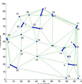
The dual of the Voronoi diagram is the Delaunay triangulation Del(S). Del(S) is geometrically realized as a triangulation of the convex hull of S (see Fig. 1). After con-structing Delaunay, we calculate the length of the three edges of each triangle. If the length of the edge is no more than transmission range Rt, then connect it. As shown in Fig. 1,
Fig. 1. An example of constructing Delaunay using 30 terminal nodes. The thin solid lines represent the edges of the Delaunay triangulation that are not connected. The initial disconnected ter-minal nodes are indicated by the ‘•’-sign. The initial connected sub-graphs are indicated by the thick solid lines.
Fig. 2. An example of Lemma 1.
Phase 2: Add relay nodes
We first illustrate the following lemmas about adding relay nodes.
Lemma 1 One relay node can connect at most five nodes that belong to different sub-
graphs [11].
Proof: We prove this lemma by contradiction. As shown in Fig. 2, if six nodes can be
covered by a minimum circle of radius R where R is no more than the transmission range
Rt, we draw a circle of radius Rt to cover the six nodes centered at o, then draw six lines
from each node to the center of the circle. Assume that the shortest length of the adjacent nodes pair (a, b) is d1. We extend the length of line (a, b) from d1 to d2. That is, nodes a and b are on the circle. If d2 is equal to Rt, each edge of triangle (a, o, b) has the same
length. Angle (a, o, b) is equal to 60°. If d2 is larger than Rt, then the angle (a, o, b) is
lar-ger than 60°. The sum of all six angles is larlar-ger than 360°. It is a contradiction. Therefore, one relay node can connect at most five nodes that belong to different sub-graphs.
(a) (b)
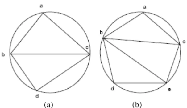
Fig. 3. (a) An example of four nodes covered by a minimum circle of radius R; (b) An example of five nodes covered by a minimum circle of radius R.
Lemma 2 Four nodes a, b, d, c can be covered by a minimum circle of radius R if and
only if all the four triangles (a, b, d), (b, d, c), (d, c, a), (c, a, b) can be covered by a minimum circle of radius R.
Proof: As shown in Fig. 3 (a), triangles (a, b, c) and (b, d, c) form a quadrilateral (a, b, d,
c). From Lemma 8 in [11], four nodes a, b, d, c can be covered by a disc of radius R if all
the four triangles (a, b, d), (b, d, c), (d, c, a) and (c, a, b) can be covered by a minimum circle of radius R.
Lemma 3 Five nodes a, b, d, e, c can be covered by a minimum circle of radius R if
and only if all the four quadrilaterals (a, b, d, e), (b, d, e, c), (d, e, c, a), (e, c, a, b) can be covered by a minimum circle of radius R.
Proof: As shown in Fig. 3 (b), each of the three adjacent triangles (c, a, b), (c, b, e) and (b,
e, d) can be covered by a minimum circle of radius R. We prove this lemma by
contradic-tion. If one of the four quadrilaterals (a, b, d, e), (b, d, e, c), (d, e, c, a) and (e, c, a, b) can not be covered by a minimum circle of radius R, say (e, c, a, b). From Lemma 2, there exists at least one triangle of the four triangles (c, a, b), (a, b, e), (b, e, c), (e, c, a) that cannot be covered by a minimum circle of radius R. Assume that the triangle is (c, a, b). This contradicts our assumption that triangle (c, a, b) can be covered by a minimum circle of radius R. Therefore, five nodes a, b, d, e, and c can be covered by a minimum circle of radius R if and only if all four quadrilaterals (a, b, d, e), (b, d, e, c), (d, e, c, a), (e, c, a, b) can be covered by a minimum circle of radius R.
After Phase 1, we divide the Delaunay triangles into three types. In Type 1, the length of all edges of the triangle is larger than Rt and smaller than 2Rt. In Type 2, the longest
edge of the triangle is at most 4Rt, while the shortest edge is larger than Rt and at most 2Rt.
The properties of triangles different from Types 1 and 2 are defined as Type 3. For the triangles of Type 1, we place the relay nodes as per the following steps. First, we place one relay node to connect five nodes that are formed by three adjacent triangles. Second, we place one relay node to connect four nodes that are formed by two adjacent triangles. Third, we place one relay node to connect three nodes of one triangle. For the triangles of Type 2, we try to place two relay nodes to connect three nodes of one triangle. For the
triangles of Type 3, we add relay nodes to connect the nearest disconnected nodes pair along the edge of the triangle.
The details of adding relay nodes in the ERSPA algorithm are illustrated as follows. (1) Find the initial sub-graphs G(Nt, E(Lt, Rt)), the maximal connected sub-graph, and the
Types 1 and 2 triangles.
(2) Find the point where adding one relay node to connect the nodes in Type 1 triangles yields the maximal increase in the performance metric. The performance metric is the number of relay sensor. Add the relay node to Nr. Maintain the new sub-graphs, and
the maximal connected sub-graph. Repeat this as long as new triangles can be con-nected.
(3) Find the point to add one relay node to connect two different sub-graphs and add the relay node to Nr.
(4) Find the point to add two relay nodes to connect three different sub-graphs and add the relay nodes to Nr.
(5) If the graph G(Nt ∪ Nr, E(Lt ∪ Lr, Rt)) is not yet connected, add relay nodes to
con-nect the nearest disconcon-nected nodes pair along the edge of the triangle.
In step 2 of Phase 2, two adjacent triangles can form a quadrilateral. For example, as shown in Fig. 1, triangle (2, 29, 15) and triangle (2, 29, 22) form a quadrilateral (2, 29, 15, 22). From Lemma 2, if the circumradius of each triangle is at most Rt, then we can place
one relay node in the center of the minimal enclosing circle that covers the four points of the quadrilateral. We select the triangles that belong to the three different sub-graphs. The triangles inside the convex hull of the initial connected sub-graphs are not required to be searched. If the circumradius of the selected triangle is at most Rt, then add a node on the
circumcenter of the triangle. The circumcenter is the intersection of the perpendicular bi-sectors of the sides of the triangle. The circumradius of a triangle is the radius of the cir-cumscribed circle. The circir-cumscribed circle of a triangle is the circle that passes through
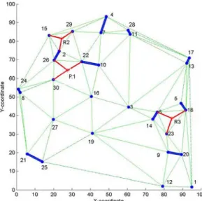
Fig. 4. An example of adding relay sensors after step 2 of Phase 2 for the ERSPA algorithm. Plac-ing one relay node to connect three nodes is indicated by the circle centered at R1, R2 and R3. The relay sensors are indicated by the ‘*’-sign.
Fig. 5. The connected sub-graphs after steps 3 and 4 of Phase 2 in the ERSPA algorithm.
the three vertices of the triangle. For example, as shown in Fig. 4, R1 is the circumcenter of the triangle (30, 26, 22). If the distance from R1 to each apex of the triangle is not lar-ger than transmission range Rt, then add a relay node R1 on the circumcenter. The relay sensors are indicated by the ‘*’-sign. The ‘•’-sign represents the initial disconnected ter-minal nodes, and the initial connected sub-graphs are represented by the thick solid line. After adding a relay node, the edge becomes connected, which is indicated by a thin solid line. The performance metric of step 2 of ERSPA is the number of relay sensor. After step 2, we place one relay node to connect two sub-graphs. For example, as shown in Fig. 5, we place one relay node R4 to connect nodes 10 and 16. After step 3, we place two relay nodes to connect three different sub-graphs. For example, as shown in Fig. 5, we place one relay node R6 to connect nodes R5 and node 3. After step 4, if the graph G(Nt ∪ Nr, E(Lt
∪ Lr, Rt)) is not yet connected, then place K relay nodes to connect two sub-graphs. Step
5 exists here to handle the case of Type 3 triangle.
The number of required relay sensors to add into the edge of the nearest pair of nodes is illustrated as Eq. (2).
K × Rt < d(u, v) ≤ (K + 1) × Rt, K = 3, …, n (2)
where K is the number of relay nodes. d(u, v) is the distance between node u and node v. For example, as shown in Fig. 4, we place two relay nodes to connect nodes 21 and 27. Repeat Phase 2 until the complete communication graph is connected (see Fig. 6).
In Phase 1, constructing Delaunay takes O(N logN) times. Steps 1-2 of Phase 2 cost
O(N) in plane and O(N2) in three-dimensional sensing space. Steps 3-5 of Phase 2 cost
O(N). Therefore, Phase 2 requires O(N) times to add relay sensors in two-dimensional
sensing space and O(N2) in three-dimensional sensing space. The total time complexity of the ERSPA algorithm is O(N2). It is feasible in a two dimensional space.
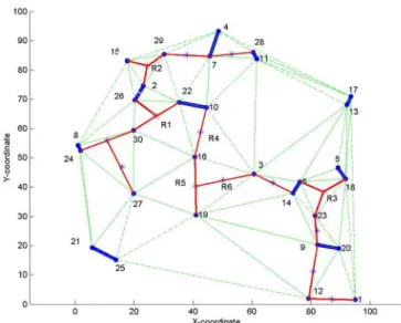
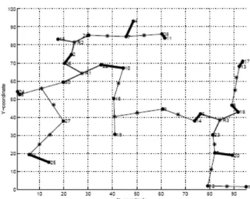
Fig. 6. The final connected communication graph. The transmission range is 10 percent of the side of the square sensing field.
4. SIMULATION RESULTS
4.1 Performance Metrics and Environment Setup
This section presents the performance analysis of the ERSPA algorithm. The metrics for performance are given as follows, (1) Average number of relay sensors: The average number of relay sensors is defined as the required minimal average number of additional sensors to make the network connected; (2) Time complexity: Time complexity is defined as the time to run the algorithm.
The environment setup of the simulation is described as follows. There are different numbers of terminal sensors randomly deployed in a 100 × 100 two-dimensional sensing area. The maximum transmission range is 10 percent of the side of the square sensing field. The network can convey location information of terminal nodes to the base station, then limit the transmission range to a bounded value Rt for energy efficiency.
4.2 Numerical Results
Comparisons of the two performance metrics were made for three schemes: the ER-SPA algorithm, the Minimum Spanning Tree (MST) algorithm and the Greedy algorithm [13]. The MST algorithm has two steps. First, it generates a minimum spanning tree to connect the terminal nodes. Then, it places the relay nodes on the edges of the minimal spanning tree that are longer than the transmission range Rt. The MST algorithm takes
O(N logN) times.
The performance metrics include the total number of relay sensors and the time com-plexity. The details are illustrated as follows,
Nt = 50, Rt= 10% Nt= 90, Rt= 10%
MST Greedy ERSPA MST Greedy ERSPA 24 20 16 12 8 4 0 average nu mber of relay n o d es 24 20 16 12 8 4 0 average numb er of rela y nodes (a) (b)
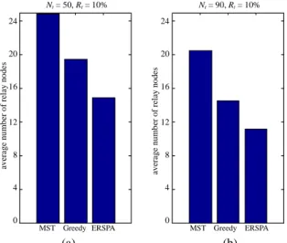
Fig. 7. (a) The average number of relay nodes for connectivity with 50 terminal nodes; (b) The average number of relay nodes for connectivity with 90 terminal nodes. The transmission range is 10 percent of the side of the square sensing field.
Nt = 30, Rt= 10% Nt= 30, Rt= 12%
MST Greedy ERSPA MST Greedy ERSPA 24 20 16 12 8 4 0 av erage num be r of re lay node s 16 12 8 4 0 ave ra g e num ber of rel ay nodes (a) (b)
Fig. 8. (a) The average number of relay nodes for connectivity with 30 terminal nodes. The trans-mission range is 10 percent of the side of the square sensing field; (b) The average number of relay nodes for connectivity with 30 terminal nodes. The transmission range is 12 percent of the side of the square sensing field.
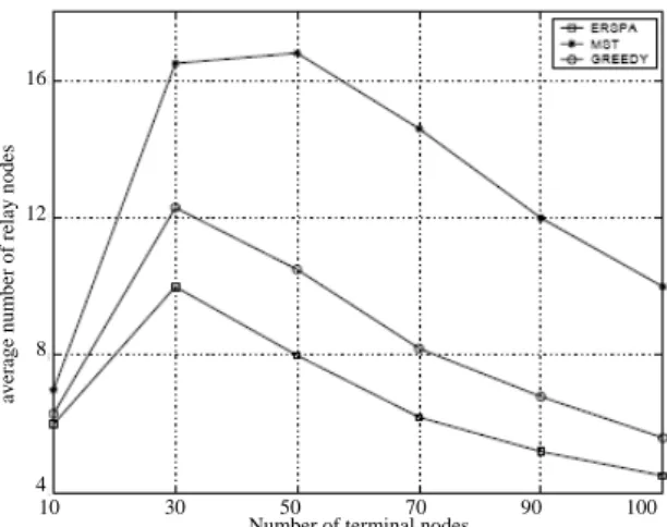
(1) Average number of relay sensors: Fig. 7 shows that the average number of relay nodes of ERSPA is smaller than that of the minimum spanning tree algorithm and the greedy algorithm with different number of terminal nodes. Fig. 8 shows that the av-erage number of relay nodes of ERSPA is smaller than the minimum spanning tree algorithm and the greedy algorithm when Nt is 30 and Rt is different. Fig. 9 shows that
the average number of ERSPA relay nodes is smaller than that of the minimum span-ning tree and the greedy algorithms under different terminal nodes when Rt is 10
relay nodes of ERSPA is also smaller than that of the minimum spanning tree and the greedy algorithms when Rt is 12 percent of the side of the square sensing field. The
average number of relay sensors in MST is approximately two times that of the ER-SPA algorithm. This is because ERER-SPA finds the optimal locations to place relay sen-sors and connects the maximal number of disconnected sub-graphs.
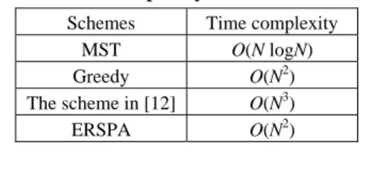
(2) Time complexity: The time complexity of ERSPA algorithm is illustrated as follows. Phase 1 costs O(N logN) times to construct Delaunay triangulations where N is the number of terminal nodes. Steps 1-2 of Phase 2 cost O(N) in plane and O(N2) in three-dimensional sensing space. Steps 3-5 of Phase 2 cost O(N). Therefore, Phase 2 requires O(N) times to add relay sensors in two-dimensional sensing space and O(N2) in three-dimensional sensing space. The total time complexity of the ERSPA algorithm is O(N2). The greedy algorithm takes O(N2) times. The minimum spanning tree takes
O(N logN) times. The scheme in [12] takes O(N3) times. The time complexity of ER-SPA is feasible in a two dimensional space.
10 30 50 70 90 100 Number of terminal nodes
24 20 16 12 8 av er ag e n u m b er o f re lay no d es
Fig. 9. The average number of relay nodes for connectivity under different terminal odes. The trans-mission range is 10 percent of the side of the square sensing field.
10 30 50 70 90 100 Number of terminal nodes
16 12 8 4 aver age nu m b er o f re lay n o d es
Fig. 10. The average number of relay nodes for connectivity under different terminal nodes. The transmission range is 12 percent of the side of the square sensing field.
Table 1. Time complexity of different schemes.
Schemes Time complexity
MST O(N logN)
Greedy O(N2)
The scheme in [12] O(N3)
ERSPA O(N2)
5. CONCLUSIONS
This paper presents an efficient relay sensor placing algorithm for connectivity in wireless sensor networks. Compared with the minimal spanning tree and the greedy algo-rithms, our ERSPA algorithm gives better performance in terms of the average number of relay sensors. This is because ERSPA places the relay sensors in optimal places to con-nect the maximum number of initial concon-nected sub-graphs such that the average number of relay sensors can be minimized. We are confident that ERSPA is an efficient and use-ful algorithm for further wireless ad hoc sensor networks.
REFERENCES
1. R. J. Wan and C. W. Yi, “Asymptotic critical transmission radius and critical neighbor number for K-connectivity in wireless ad hoc networks,” in Proceedings of the 5th
ACM International Symposium on Mobile Ad Hoc Networking and Computing, 2004,
pp. 1-8.
2. P. Santi, “The critical transmitting range for connectivity in mobile ad hoc networks,”
IEEE Transactions on Mobile Computing, Vol. 4, 2005, pp. 310-317.
3. H. Koskinen, “A simulation-based method for predicting connectivity in wireless multihop networks,” Telecommunication Systems, Vol. 26, 2004, pp. 321-338. 4. H. Zhang and J. C. Hou, “Maintain sensing coverage and connectivity in large sensor
networks,” Ad Hoc and Sensor Networks, Vol. 1, 2005, pp. 89-124.
5. D. Tian and N. D. Georganas, “Connectivity maintence and coverage reservation in wireless sensor networks,” Ad Hoc Networks, Vol. 3, 2005, pp. 744-761.
6. H. Gupta, S. R. Das, and Q. Gu, “Connected sensor cover: Self-organization of sensor networks for efficient query execution,” in Proceedings of ACM Symposium on
Mo-bile Ad Hoc Networking and Computing, 2003, http://www.cs.sunysb.edu/~hgupta/
ps/coverage-mobihoc-2003.pdf.
7. X. Wang, G. Xing, Y. Zhang, C. Lu, R. Pless, and C. Gill, “Integrated coverage and connectivity configuration in wireless sensor networks,” in Proceedings of the 1st
In-ternational Conference on Embedded Networked Sensor Systems, 2003, pp. 28-39.
8. X. Cheng, D. Z. Du, L. Wang, and B. Xu, “Relay sensor placement in wireless sen-sor networks,” IEEE Transactions on Computers, Vol. 56, 2001, pp. 1-19.
9. E. L. Lloyd and G. Hue, “Relay node placement in wireless sensor networks,” IEEE
Transactions on Computers, Vol. 58, 2007, pp. 134-138.
10. I. Mandoiu and A. Zelikovsky, “A note on the MST heuristic for bounded edge- length Steiner trees with minimum number of Steiner points,” Information
Process-ing Letters, Vol. 69, 1999, pp. 53-57.
11. D. Chen, D. Z. Du, X. Xu, G. H. Lin, L. Wan, and G. Xue, “Approximations for Steiner trees with minimum number of Steiner points,” Journal of Global Optimization, Vol. 18, 2000, pp. 17-33.
12. X. Cheng, D. Z. Du, L. Wang, and B. Xu, “Relay sensor placement in wireless sensor networks,” Wireless Networks, Vol. 14, 2008, pp. 347-355.
13. Y. T. Hou, Y. Shi, H. D. Sherali, and S. F. Midkiff, “On energy provisioning and relay node placement for wireless sensor networks,” IEEE Transactions on Wireless
Communications, Vol. 4, 2005, pp. 2579-2590.
14. H. Koskinen, J. Karvo, and O. Apilo, “On improving connectivity of static ad-hoc net-works by adding nodes,” Med-Hoc-Net, 2005, pp. 169-178.
15. D. Ganesan, R. Christescu, and B. B. Lozano, “Power-efficient sensor placement and transmission structure for data gathering under distortion constrain,” ACM
Transac-tions on Sensor Networks, Vol. 2, 2006, pp. 155-181.
16. K. Mulmuley, Computational Geometry, Prentice Hall, Englewood Cliffs, NJ, 1994.
Jyh-Huei Chang (張志輝) received his M.S. degree in Computer Science from Na-tional Chiao Tung University, Taiwan in 2002. He is currently working toward the Ph.D. degree in Computer Science at National Chiao Tung University, Taiwan. He is a Ph.D. candidate now. His research interests include wireless networks, wireless sensor networks and mobile computing.