針對多重天線架構下的無線網狀網路計算其輸出上限之演算法研究

國

立

交

通

大

學

網路工程研究所

 

碩 士 論 文

       

針對多重天線架構下的無線網狀網路計算其

輸出上限之演算法研究

An Upper Bound of the Throughput for Multi-Radio

Wireless Mesh Networks

     

研 究 生：黃淑盈

指導教授：簡榮宏 教授

     

中 華 民 國 九 十 八 年 七 月

針對多重天線架構下的無線網狀網路計算其輸出上限之演算法

研究

An Upper Bound of the Throughput for Multi-Radio Wireless Mesh

Networks

 

 

 

研 究 生：黃淑盈 Student：Shu-Ying Huang

指導教授：簡榮宏 Advisor：Rong-Hong Jan

 

 

 

國 立 交 通 大 學

網 路 工 程 研 究 所

碩 士 論 文

A Thesis

Submitted to Institute of Network Engineering College of Computer Science

National Chiao Tung University in partial Fulfillment of the Requirements

for the Degree of Master

in

Computer Science

July 2009

Hsinchu, Taiwan, Republic of China

針對多重天線架構下的無線網狀網路計

算其輸出上限之演算法研究

研究生：黃淑盈      指導教授：簡榮宏  博士 

 

 

 

國立交通大學網路工程研究所

 

 

摘   

 

要 

  無線網狀網路是由網狀節點以及網狀用戶端所組成。網狀節點以無線 方式彼此連結形成網狀骨幹網路以提供網狀用戶端存取網際網路資訊。在 本篇論文中，我們針對沒有訊號干擾的情況之下，給定每一個網狀節點的 位置以及每一個網狀節點所配置的天線個數計算從網狀用戶端到網際網路 入口的最大網路輸出值。我們將這個最大網路輸出值定義成該網路的輸出 上限值。在本篇論文中，我們提出了一個演算法來解網路輸出上限的問題。 我們的方法是將上述的問題轉換成最大流量問題。如此一來就可以透過最 大流量演算法來求解，所花的計算時間椱雜度和多項式成比例。除此之外， 我們利用模擬的方法，探討不同的因素包括網狀節點所放置的位置、網狀 閘道節點的個數以及網狀節點所配置的天線個數對輸出上限值的影響。    

An Upper Bound of the Throughput

for Multi-Radio Wireless Mesh

Networks

Student: Shu-Ying Huang

Advisor: Dr. Rong-Hong Jan

INSTITUTE OF NETWORK ENGINEERING

NATIONAL CHIAO TUNG UNIVERSITY

Abstract

A wireless mesh network consists of mesh routers and mesh clients. Mesh routers form the wireless backbone through wireless links which provides mesh clients connecting to the wired Internet. In this thesis, we consider the following problem: given a deployment of mesh routers and the number of radio interfaces of each mesh router, what is the maximum throughput from mesh clients to the wired Internet under interference-free assumption. We define the maximum throughput of the problem as an upper bound of the throughput for the given wireless mesh network. The proposed problem is transformed into a maximum flow problem and then the problem can be solved by existing maximum flow algorithms. Therefore, an upper bound of the throughput for the given wireless mesh network can be obtained in polynomial time. The simulation results show that the upper bound of the throughput is affected by the deployment of mesh routers, the number of mesh routers which serve as gateway and the number of radio interfaces of each mesh router.

致謝

首先我要先感謝我的指導教授簡榮宏老師，在老師的教導下使我對無 線網路的領域有更深入的了解。除此之外，透過老師的指導讓我學會了如 何明確的定義問題以及正確的解決問題，進而使得本篇論文得以產生。同 時也是由於老師的協助才能使得本篇論文能夠更加的完整而嚴謹。 接著我要感謝實驗室裡的學長姐(安凱、嘉泰、蕙如、鈺翔、奇育、家 瑋、文彬、敬之、宇翔、允琳、佑笙、俊傑)、同學(志賢、子興)以及學弟 妹們(嘉瑋、宇田)讓我的這兩年的研究生生活變得多采多姿，尤其是實驗室 的共同出遊更讓我留下美好的回憶。感謝安凱學長百忙之中能指導我如何 了解一篇論文的重點以及如何報告。 最後要感謝我的家人和朋友，謝謝你們的關心以及鼓勵，使我能夠順 利的完成碩士的學位。

Content

1 Introduction ...1 2 Related Work ...4 3 Problem Definition ...7 3.1 Network Model...7 3.2 Problem Definition ...8 4 Problem Transformation...14

4.1 Transformation Problem P1 into a Maximum Flow Problem ...14

4.2 Illustrated Examples ...20

5 Time Complexity and Numerical Results ...24

5.1 Time Complexity...24

5.2 Numerical Results ...24

6 Conclusion and Future Work ...27

References ...28                            

List of Figures

 

Figure 3.1 A network architecture ...8

Figure 3.2 A graph representing the upload netwok flow ...9

Figure 3.3 The capacity of graph...10

Figure 3.4 The flow on graph ...12

Figure 4.1 A transformation for pure router ...15

Figure 4.2 A transformation for mesh gateway ...17

Figure 4.3 A transformation for mesh AP ...19

Figure 4.4 Example 1 ...21

Figure 4.5 Example 2 ...22

Figure 4.6 Example 3 ...23

Figure 5.1 Throughput upper bound v.s. topology number ...25

Figure 5.2 Throughput upper bound v.s. number of mesh gateways ...26

Figure 5.3 Throughput upper bound v.s. number of backhaul interfaces...26

 

 

List of Tables

  Table 3.1 Meanings of symbols...8

 

Chapter 1

Introduction

A wireless mesh network consists of mesh routers and mesh clients where mesh routers have minimal mobility and form the wireless backbone through wireless links. Other than the routing functionality, mesh routers contains additional functions to support mesh networking. With access point functionality, mesh routers can provide network access for mesh clients within their coverage area. With gateway functionality, mesh routers can connect to the wired Internet [1]. In such networks, traffic is mainly routed by the mesh routers between the mesh clients and the wired Internet.

Wireless mesh networks are attractive to several wireless network applications, e.g., wireless last mile access of ISPs, broadband home networking, community and neighborhood networks, enterprise networking, building automation, and so on. The main reason is the low cost of deployment and maintenance due to the absence of a wired infrastructure. However, wireless communication suffers from interference problem which prohibits simultaneous transmissions in a common neighborhood.

The wireless interference can be alleviated if different node pairs in a common neighborhood use different non-overlapping channels. Fortunately, the IEEE 802.11b/g standard provides 3 non-overlapping channels in the 2.4 GHz spectrum and IEEE 802.11a standard provides 12 non-overlapping channels in the 5 GHz spectrum. However, a single-radio wireless mesh network, i.e., to

equip each mesh router with one radio interface, forces all routers to use the same channel to maintain network connectivity. This architecture poorly utilizes available spectrum and suffers from the well-known capacity scaling problem [12], [13].

We therefore consider a multi-radio wireless mesh network, i.e., to equip each mesh router with multiple radio interfaces, for effective use of available orthogonal channels. This architecture allows multiple simultaneous transmissions within a common neighborhood as long as different radio interface pairs which used for transmissions work on different non-overlapping channels. Thus, it can reduce the wireless interference and increase the network throughput [4], [10].

Two of the most challenging research issues in multi-radio wireless mesh networks are the channel assignment and the routing problems. The channel assignment problem determines an assignment of channels to radio interfaces, while the routing problem determines the routing paths for the flow from source to destination and thus determines the flow on each link. The goal of these two problems is to maximize the network throughput. Unfortunately, the problem of finding optimal throughput is NP-hard [12].

In this thesis, we want to find an upper bound of the throughput for multi-radio wireless mesh networks. More precisely, our problem is that given the deployment of mesh routers and the number of radio interfaces of each mesh router, we want to find the maximum flow from mesh clients to the wired Internet under interference-free assumption. We define the maximum throughput of the problem as an upper bound of the throughput for the given wireless mesh network. Because we assume that interference does not arise and radio interfaces equipped at each router are set to different non-overlapping channels, the capacity of each router is equal to its radio interfaces multiplied by channel capacity. Therefore, for each mesh router, the sum of incoming flows plus the sum of outgoing flows cannot exceed the mesh router’s capacity. We

proposed a transformation method which transforms the proposed problem into a maximum flow problem [14] and then solved it by the existing maximum flow algorithms, e.g., Ford-Fulkerson algorithm [15], Edmonds-Karp algorithm [16], Dinic’s algorithm [17], etc. The contributions of this thesis are listed in the following:

‧ We show that the proposed problem can be solved in polynomial time. In

other words, we can obtain an upper bound of the throughput for the wireless mesh network in polynomial time.

‧ We show that the deployment of mesh routers, the number of mesh routers

which serve as gateway and the number of radio interfaces of each mesh router affect the upper bound of the network throughput.

‧ The resulting flow, i.e., the maximum flow, can provide the basis for

channel assignment, i.e., to assign channels to radio interfaces based on the flow on each link.

Chapter 2

Related Work

The maximum flow problem is to find a feasible flow from the source to the sink in a flow network that is maximized. The maximum flow problem can be mathematically defined as follows. Consider a flow network

which is a directed graph where each edge

) , (V E G= E j i, )∈ ( has a nonnegative

capacity . We distinguish two nodes in the flow network: a source and a sink . A flow in must satisfy the following properties:

0 ≥ ij c s t G V i t i if f t i s i if s i if f x x V k ki V j ij ∀ ∈ ⎪ ⎩ ⎪ ⎨ ⎧ = − ≠ ∧ ≠ = = −

∑

∑

∈ ∈ , , 0 , (1) V j i c x_ij ≤ _ij ∀ ∈ ≤ , , 0 (2) Constraint (1) ensures that for each node, except the source and the sink, the sum of incoming flows is equal to the sum of outgoing flows. Constraint (2) ensures that the flow on each link cannot exceed the capacity of the edge and the flow on each edge is non-negative. Given a flow network with source and sink t, a maximum flow problem is to find a flow from to t

with maximum value without violating above constraints. This problem can be solved by several efficient algorithms, i.e., Ford-Fulkerson algorithm, Edmonds-Karp algorithm, Dinic’s algorithm, etc.

) , (V E

G=

s s

Several studies [2]-[10] have been proposed for multi-radio wireless mesh networks. In [2] and [3], the authors proposed a flow rate computation method

to find a maximum flow from mesh clients to the wired Internet in the absence of wireless interference. Because of maximizing the network flow, this method is not dependent on any particular traffic profile. The authors assume that mesh routers have to forward packets toward the wired network, regardless of which particular gateway is used. In other words, mesh aggregation devices collecting user traffic do not have to forward each packet to a specific mesh gateway, but can direct it to any of the mesh gateways. In this assumption, the problem of maximizing the flow from any source to any sink is a single commodity flow problem with multiple sources and sinks. There is a standard trick to reduce this more general version to the case with a single source and a single sink by adding two extra nodes. That is, two nodes s and t are added to connect to the nodes in and , respectively, with links of infinite capacity, where is the set of mesh aggregation devices and is the set of mesh gateways.

A

V V_G VA

G

V

In [4], the authors proposed 802.11-based multi-channel wireless mesh network architecture and developed an iterative approach to solve the joint routing and channel assignment problem. The goal is to maximize the cross-section goodput over all the source-destination pairs in the network. They start with an initial estimation of the expected load on each virtual link without regard to the link capacity, and then iterate over channel assignment and routing steps until the bandwidth allocated to each virtual link matches its expected load as closely as it can. In [5], the authors presented an algorithm to finds the optimal routes for a given objective of meeting a set of demands in the network using a set of necessary conditions as constraints. They also proposed two link channel assignment algorithms which allow us to schedule flows on the links in the network. In [6], the authors rigorously formulated the joint channel assignment and routing problem as an integer linear program (ILP). Since the ILP problem is NP-hard, they first solve a linear program relaxation of the joint problem. This result provides the flow on the flow graph along with a not necessarily feasible channel assignment for the node radios. The channel

assignment algorithm aims to fix this feasibility. The flow on the graph is then readjusted and scaled to ensure a feasible channel assignment and routing. Besides, a scheduling algorithm is used to produce an interference free link schedule. The goal is to maximize the bandwidth allocated to each traffic aggregation point subject to fairness constraint. In [7] and [8], the proposed channel assignment and routing schemes take into account both network efficiency and fairness, i.e., max-min fairness and proportional fairness. In [9], they balance the load among logical links and provide higher effective capacity for the bottleneck links in wireless mesh networks. In [10] and [11], the authors proposed distributed algorithms to dynamically adjust channel assignment and routing.

Chapter 3

Problem Definition

3.1 Network

Model

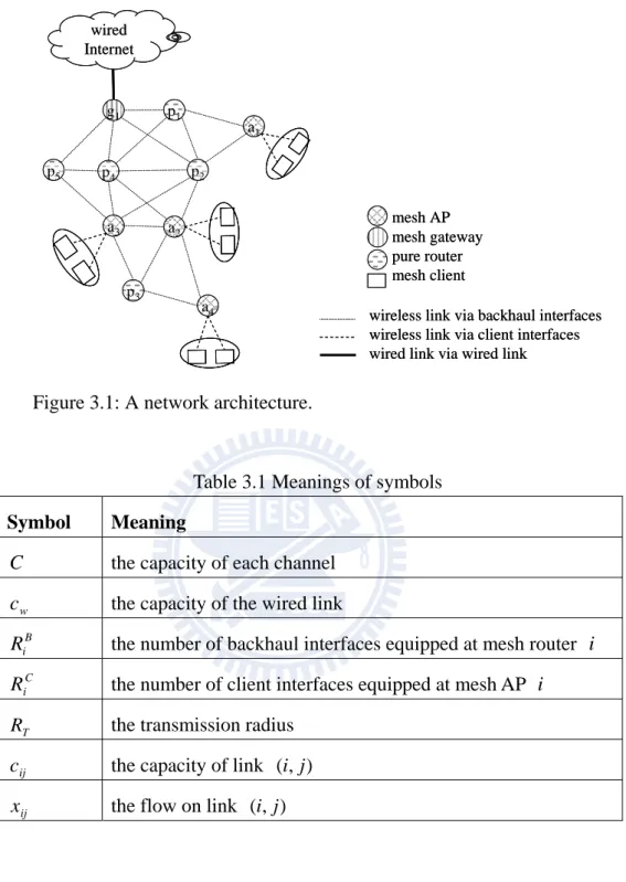
In this thesis, we consider the multi-radio wireless mesh network architecture as shown in Figure 3.1. There are three types of mesh routers, i.e., pure routers, mesh gateways and mesh APs. All of them are equipped with backhaul interfaces which are used for backbone communication. Besides backhaul interfaces, each mesh gateway is equipped with gateway functionality to enable connectivity to the wired Internet via wired link e.g., high-speed Ethernet and each mesh AP is equipped with client interfaces which are used for providing network access for mesh clients within their coverage area. We assume that every mesh router i is equipped with backhaul

interfaces and every mesh AP is equipped with client

interfaces. We also assume that all backhaul interfaces have identical transmission radii (denoted by ). The sets of the pure routers, the mesh gateways and the mesh APs are denoted as , and , respectively..

) 1 ( _iB ≥ B i R R i R_iC (R_iC ≥1) T R P V V_G VA

p5 p4 a₁ p₁ a₂ p₃ g₁ a4 p2 a₃ wired Internet p5 p4 a₁ p₁ a₂ p₃ g₁ a4 p2 a₃ wired Internet mesh AP mesh gateway pure router mesh client mesh AP mesh gateway pure router mesh client

wireless link via backhaul inte wireless link via client interfaces wired link via wired link

rfaces wireless link via backhaul inte wireless link via client interfaces wired link via wired link

rfaces

Figure 3.1: A network architecture.

Table 3.1 Meanings of symbols

Symbol Meaning

C the capacity of each channel

w

c the capacity of the wired link

B i

R the number of backhaul interfaces equipped at mesh router i

C i

R the number of client interfaces equipped at mesh AP i

T

R the transmission radius

ij

c the capacity of link ( ji, )

ij

x the flow on link ( ji, )

3.2 Problem

Definition

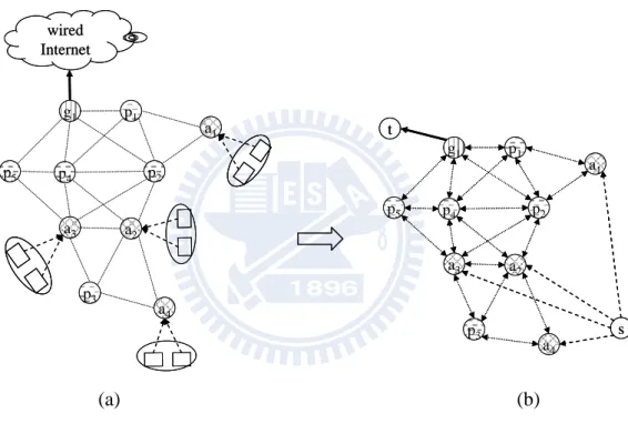
In this thesis we want to find a maximum flow from mesh clients to the wired Internet in the wireless mesh network under interference-free assumption (see Figure 3.2(a)).We model the considered wireless mesh network as a directed graph G =(V,E) shown in Figure 3.2(b), where V is a set of nodes

containing all mesh routers plus a source and a sink t. The source represents all mesh clients and the sink represents the wired Internet. Given any two mesh routers, if the distance between them is less than transmission

s s

t

radius, there are two directed edges with opposite directions between them. We add an edge from to every mesh AP and also add an edge from every mesh gateway to . Formally, the edge set

s t {(i, )| }, } | ) , {( } , }, , { , | ) , {(i j i j V s t i j d_ij R_T s i i V_A t i V_G E = ∈ − ≠ ≤ ∪ ∈ ∪ ∈

where d_ij is the distance between and . i j

wired Internet

Figure 3.2: (a) The network flow from mesh clients to the wired Internet. (b) The corresponding graph G=(V,E), where represents all mesh clients and

represents the wired Internet.

s t

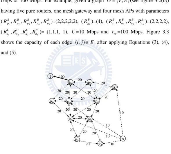
We assign an edge capacity c_ij for each edge (i, j)∈E as follows.

t j s i E j i C R C R c_ij =min( _iB × , _jB× ), ∀( , )∈ ∧ ≠ ∧ ≠ (3) E i s C R c_si = _iC× , ∀( , )∈ (4) E t i c c_it = _w, ∀( , )∈ (5) where is the number of backhaul interfaces of mesh router , is the number of client interfaces of mesh AP , is the capacity of the

) ( B_j B i R R i( j) C i R i c_w (a) (b) p₅ p4 a₁ p₁ a₂ p₃ g1 a₄ p₂ a₃ wired Internet p₁ g1 p₅ p4 a₁ a₂ p₃ a₄ p₂ a₃ t p5 p4 a₁ p₁ a₂ p₃ g₁ a4 p2 a₃ s t p₁ g₁ a₁ p5 p4 p2 a₃ a₂ s p₃ a4

wired link and is the channel capacity. In Equation (3), is the maximum capacity of mesh router and thus we set the capacity of

edge between two mesh routers to the minimum value of

. In Equation (4), we set the capacity of the edge to the number of client interfaces of mesh AP multiplied by channel capacity. In Equation (5), we set the capacity of the edge to the capacity of the wired link. The wired link can be a high-speed Ethernet and it’s capacity can be 1 Gbps or 100 Mbps. For example, given a graph

C R_iB×C(RB_j ×C) ) ( j i j i, ) , (R_iB×C RB_j ×C ( is, ) i ) , ( ti ) , (V E G = (see figure 3.2(b)) having five pure routers, one mesh gateway and four mesh APs with parameters

( , , , , )=(2,2,2,2,2), ( )=(4), ( , , , )=(2,2,2,2),

( , , , )= (1,1,1, 1), =10 Mbps and =100 Mbps. Figure 3.3

shows the capacity of each edge

B p R 1 B p R 2 B p R 3 B p R 4 B p R 5 B g R 1 B a R 1 B a R 2 B a R 3 B a R 4 C a R 1 C a R 2 C a R 3 C a R 4 C cw E j i, )∈

( after applying Equations (3), (4), and (5). p₅ p₄ a₁ p₁ a₂ p₃ g₁ a4 p₂ a3 s t 20 20 20 20 20 20 20 20 20 20 20 20 20 20 20 20 20 20 20 ₂₀ 10 10 10 10 100 p₅ p₄ a₁ p₁ a₂ p₃ g₁ a4 p₂ a3 s t 20 20 20 20 20 20 20 20 20 20 20 20 20 20 20 20 20 20 20 ₂₀ 10 10 10 10 100

Figure 3.3: The capacity for all edge in G.

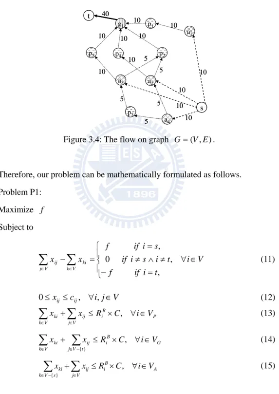
Next, we are going to formulate the proposed problem. The flow on must satisfy two basic constraints as follows. Let denote the flow on edge

. G ij x ) , ( ji

V i t i if f t i s i if s i if f x x V k ki V j ij ∀ ∈ ⎪ ⎩ ⎪ ⎨ ⎧ = − ≠ ∧ ≠ = = −

∑

∑

∈ ∈ , , 0 , (6) V j i c x_ij ≤ _ij ∀ ∈ ≤ , , 0 (7) Constraint (6) ensures that for each node, except the source and the sink, the sum of incoming flows is equal to the sum of outgoing flows. Constraint (7) ensures that the flow on each link cannot exceed the capacity of the edge and the flow on each edge is non-negative. Then, consider the constraint of node’s capacity. For each mesh router, the sum of incoming flows and the sum of outgoing flows must not exceed its capacity, i.e., its backhaul interfaces multiplied by channel capacity. Therefore, we add three constraints as follows:

P B i V j ij V k ki x R C i V x +

∑

≤ × ∀ ∈

∑

∈ ∈ , (8) G B i t V j ij V k ki x R C i V x +

∑

≤ × ∀ ∈

∑

− ∈ ∈ , } { (9) A B i V j ij s V k ki x R C i V x +

∑

≤ × ∀ ∈

∑

∈ − ∈ , } { (10)

Constraint (8) ensures that for each pure router, the sum of incoming flows and the sum of outgoing flows cannot exceed its capacity. Constraint (9) ensures that for each mesh gateway, the sum of incoming flows and the sum of outgoing flows, except the flow to , cannot exceed its capacity. Note that constraint (9) does not consider the flow from mesh gateway to sink because the flow goes through the wired link. Constraint (10) ensures that for each mesh AP, the sum of incoming flows, except the flow from , and the sum of outgoing flows cannot exceed its capacity. Similarly, constraint (10) does not consider the flow from source to mesh AP because the flow goes through mesh APs’ client interfaces. For example, given a graph

t t s s ) , (V E

G = (see figure 3.3) having five pure routers, one mesh gateway and four mesh APs with parameters

( , , , , )=(2,2,2,2,2), ( )=(4), ( , , , )=(2,2,2,2), ( , , , )=(1,1,1,1), =10 Mbps and =100 B p R 1 B p R 2 B p R 3 B p R 4 B p R 5 B g R 1 B a R 1 B a R 2 B a R 3 B a R 4 C a R 1 C a R 2 C a R 3 C a R 4 C cw

Mbps, and the capacity of each edge was applied by Equations (3), (4), and (5). Figure 3.4 shows an example of a feasible flow which satisfies above flow constraints and the total flow out of source is 40Mbps. The goal of our problem is to maximize the total flow out of source.

p₅ p₄ a₁ p₁ a2 p3 g₁ a4 p₂ a₃ 10 10 10 10 10 10 10 5 10 10 10 5 5 5 5 10 40 s t p₅ p₄ a₁ p₁ a2 p3 g₁ a4 p₂ a₃ 10 10 10 10 10 10 10 5 10 10 10 5 5 5 5 10 40 s t

Figure 3.4: The flow on graph G=(V,E).

Therefore, our problem can be mathematically formulated as follows. Problem P1: Maximize f Subject to V i t i if f t i s i if s i if f x x V k ki V j ij ∀ ∈ ⎪ ⎩ ⎪ ⎨ ⎧ = − ≠ ∧ ≠ = = −

∑

∑

∈ ∈ , , 0 , (11) V j i c x_ij ≤ _ij ∀ ∈ ≤ , , 0 (12) P B i V j ij V k ki x R C i V x +

∑

≤ × ∀ ∈

∑

∈ ∈ , (13) G B i t V j ij V k ki x R C i V x +

∑

≤ × ∀ ∈

∑

− ∈ ∈ , } { (14) A B i V j ij s V k ki x R C i V x +

∑

≤ × ∀ ∈

∑

∈ − ∈ , } { (15)

There are several efficient commercial software packages (e.g., CPLEX [18]) that can be applied to solve Problem P1. Most of them use the branch-and-cut algorithm [19]. However, these packages only solve Problem P1 easily in small scale networks. For large-scale networks, finding the optimal solutions for Problem P1 is not trivial.

Chapter 4

Problem Transformation

4.1 Transforming Problem P1 into a

Maximum Flow Problem

In this section, we present how to transform Problem P1 into a maximum flow problem. Comparing Problem P1 to the maximum flow problem, Problem P1 has additional constraints (13)-(15). In the following, we present a transformation method to transform the constraints (13)-(15) into a set of flow conservation constraints and edge capacity constraints.

1) We can rewrite constraint (13) as follows.

P B i V j ij V k ki x R C i V x +

∑

≤ × ∀ ∈

∑

∈ ∈ , )) 11 ( ( , i V byconstraint C R x x _iB _P V k ki V k ki+ ≤ × ∀ ∈ ⇒

∑

∑

∈ ∈ P B i V k ki R C i V x ≤ × ∀ ∈ × ⇒

∑

∈ , 2 P B i V k ki R C i V x ≤ × ∀ ∈ ⇒

∑

∈ , 2 / ) ( (16)

Let flow

∑

∈ = V k ki i i x x out in)( ) ( ' . (17)

Inequation (16) can be rewritten as

P B i i i R C i V x out in ≤( × )/2,∀ ∈ ' ) ( ) ( (18)

Equation (17) can be rewritten as

0 ' ) ( ) ( −

∑

= ∈V k ki i i x x out in (19)

By constraint (11), equation (17) can be rewritten as

0 ' ) ( ) ( = −

∑

∈V iiniout j ij x x (20)

Thus, constraint (13) can be replaced by two flow conservation constraints (constraints (19) and (20)) and an edge capacity constraint (constraint (18)).

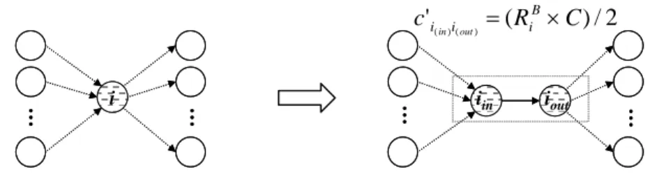
The above transformation can be explained as follows. We split each pure router into and . The node has an edge entering it for every

edge entering . The node has an edge leaving it for every edge

leaving . We add one edge connecting and directed towards

and set the capacity of edge to . See Figure 4.1.

i i_in i_out i_in

i i_out

i i_in i_out

out

i (i_in,i_out) (R_iB×C)/2

Figure 4.1: a transformation for pure router. 2 / ) ( ' ) ( ) ( R C ci_ini_out = iB× … … i … … i …… ii_inin ii_outout ……

2) Constraint (14) can be transformed as follows. G B i t V j ij V k ki x R C i V x +

∑

≤ × ∀ ∈

∑

− ∈ ∈ , } { )) 11 ( ( , } { nt constrai by V i C R x x B _G i t V j ij V j ij + ≤ × ∀ ∈ ⇒

∑

∑

− ∈ ∈ G B i t V j ij t V j ij it x x R C i V x + + ≤ × ∀ ∈ ⇒

∑

∑

− ∈ − ∈ , ) ( } { } { G B i t V j ij it x R C i V x + × ≤ × ∀ ∈ ⇒

∑

− ∈ , 2 } { G it B i t V j ij R C x i V x ≤ × − ∀ ∈ ⇒

∑

− ∈ , 2 / ) ( } { (21)

Note that x_it ≤min(c_it,R_iB×C)

Then, inequation (21) can be rewritten as

G B i it B i t V j ij R C c R C i V x ≤ × − × ∀ ∈

∑

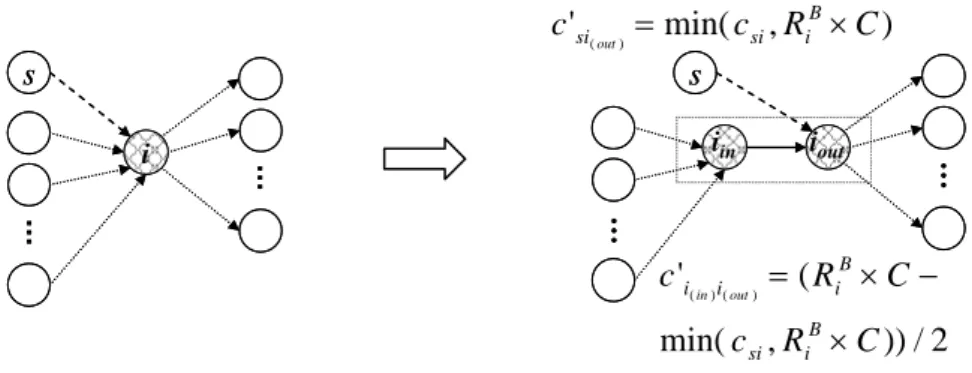
− ∈ , 2 / )) , min( ( } {

Similarly, let two flows

∑

− ∈ = } { ) ( ) ( ' t V j ij i i x x in out , x'i_(in)t =xit.

We replace constraint (14) by a capacity constraint

G B i it B i i i R C c R C i V x' (in)(out)≤( × −min( , × ))/2,∀ ∈

and two flow conservation constraints

0 ' ( )( ) } { = −

∑

− ∈ out ini i t V j ij x x 0 ) ( ) ' ' ( ) ' ' ( } { ) ( ) ( ) ( ) ( ) ( ) ( = + − + = − +

∑

∑

− ∈ ∈ t V j ij it i i t i V k ki i i t i x x x x x x x out in in out in in

That is, we split each mesh gateway into and . The node

has an edge entering it for every edge entering plus the edge .

i iin iout iin

The node has an edge leaving it for every edge leaving except the

edge . We set the capacity of the edge to .

We add one edge connecting and directed towards and set

the capacity of edge to . See

Figure 4.2. out i i ) , ( ti (i_in,t) min(c_it,R_iB×C) in i i_out i_out ) , (i_in i_out (R_iB×C−min(c_it,R_iB×C))/2 2 / )) , min( ( ' ) ( ) ( C R c C R c B i it B i i iin out × − × = , min( ' ) ( c R c_{i t it i}B in = ×C) i … … t i … … t … i_in i_out t … i_in i_out

Figure 4.2: a transformation for mesh gateway.

3) Similarly, constraint (15) can be transformed by two flow conservation

constraints and a capacity constraint as follows.

A B i V j ij s V k ki x R C i V x +

∑

≤ × ∀ ∈

∑

∈ − ∈ , } { )) 11 ( ( , } { on conservati by V i C R x x A B i V k ki s V k ki + ≤ × ∀ ∈ ⇒

∑

∑

∈ − ∈ A B i s V k ki si s V k ki x x R C i V x + + ≤ × ∀ ∈ ⇒

∑

∑

− ∈ − ∈ , ) ( } { } { A B i s V k ki si x R C i V x + × ≤ × ∀ ∈ ⇒

∑

− ∈ , 2 } { A si B i s V k ki R C x i V x ≤ × − ∀ ∈ ⇒

∑

− ∈ , 2 / ) ( } { (22) … t …

Note that x_si ≤min(c_si,R_iB×C)

Then, inequation (22) can be rewritten as

A B i si B i s V k ki R C c R C i V x ≤ × − × ∀ ∈

∑

− ∈ , 2 / )) , min( ( } {

Similarly, let two flows

∑

− ∈ = } { ) ( ) ( ' s V k ki i i x x in out , x'si_(out) = xsi.

We replace constraint (15) by a capacity constraint

A B i si B i i i R C c R C i V x' (in)(out)≤( × −min( , × ))/2,∀ ∈

and two flow conservation constraints

0 ' } { ) ( ) ( −

∑

= − ∈V s k ki i i x x in out 0 ) ' ' ( ) ( ) ' ' ( ) ( ) ( ) ( ) ( ) ( ) ( } { = + − + = + −

∑

∑

− ∈ ∈ out in out out in out i i si s V k ki si i i si V j ij x x x x x x x

That is, we split each mesh AP into and . The node has an

edge entering it for every edge entering except the edge . The

node has an edge leaving it for every edge leaving plus the edge

. We set the capacity of the edge to . We

add one edge connecting and directed towards and set the

capacity of edge to . See Figure

4.3. i i_in i_out i_in i ( is, ) out i i ) ,

(s i_out (s,i_out) min(c_si,R_iB×C)

in

i i_out i_out

) ,

Figure 4.3: a transformation for mesh AP.

Therefore, we construct a new graph G'=(V',E') from the original graph as follows. ) , (V E G= } , { }} , { | , { ' i i i V s t s t V = _{in out} ∈ − ∪ }} , { | ) , {( } ) , ( | ) , {( } ) , ( | ) , {( } ) , ( | ) , {( ' t s V i i i E t i t i E i s i s t j s i E j i j i E out in in out in out − ∈ ∪ ∈ ∪ ∈ ∪ ≠ ∧ ≠ ∧ ∈ = E t i C R c C R c c E i s C R C R C R c c t j s i E j i C R C R c c B i w B i it t i B i C i B i si si B j B i ij j i in out in out ∈ ∀ × = × = ∈ ∀ × × = × = ≠ ∧ ≠ ∧ ∈ ∀ × × = = ) , ( ), , min( ) , min( ' ) , ( ), , min( ) , min( ' ) , ( ), , min( ' ) ( ) ( ) ( ) ( ⎪ ⎪ ⎪ ⎪ ⎩ ⎪ ⎪ ⎪ ⎪ ⎨ ⎧ ∈ ∀ × × − × = × − × ∈ ∀ × − × = × − × ∈ ∀ × = A B i C i B i B i si B i G B i w B i B i it B i P B i i i V i C R C R C R C R c C R V i C R c C R C R c C R V i C R c out in , 2 / )) , min( ( 2 / )) , min( ( , 2 / )) , min( ( 2 / )) , min( ( , 2 / ) ( ' ) ( ) ( 2 / − )) , min( ( ' ) ( ) ( C R c C R c B i si B i i i_{in out} × × = ) , min( ' ) ( c R C c B i si siout = × … i … s … i … s … s iin iout … … s iin iout _…

The Problem P1 can be transformed into a maximum problem as follows. Pro blem P2: Maximize f Subject to ' , , 0 , ' ' ' ' V i t i if f t i s i if s i if f x x V k ki V j ij ∀ ∈ ⎪ ⎩ ⎪ ⎨ ⎧ = − ≠ ∧ ≠ = = −

∑

∑

∈ ∈ ' , , ' ' 0≤ xij≤cij ∀i j∈V

The Problem P1 can be solved through running a maximum flow algorithm on

4.2 Illustrated

Examples

In this section, we give some examples to show how to transfer the original gra

E

new graph G'=(V',E').

ph to the corresponding graph, how to find a maximum flow for the corresponding graph and how to convert the resulting maximum flow to an optimal flow for the original problem.

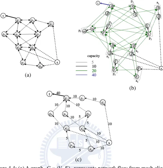
Example 1: Given a graph G =(V, ) representing the network flow from

mes e Figu

)=(1,1,1,1),

The Figure 4.4(b) gives the transform aph

h clients to the wired Internet (se re 4.4(a)). There are five pure routers, one mesh gateway and four mesh APs with parameters (R_pB 1, B p R 2, B p R 3, B p R 4, B p R 5)=(2,2,2,2,2), ( B g R 1)=(4), ( B a R 1, B a R 2, B a R 3, B a R 4)=(2,2,2,2), ed new gr (R_aC 1, C a R 2, C a R 3, C a R 4 C =10 Mbps, and c =100 Mbps. w ) ' , ' ( ' V E G = with edge

capacity. We find a maximum flow through running Edmonds-Karp algorithm [16] on Figure 4.4(b) and then convert the resulting flow to the original graph

) , (V E

G= . Figure 4.4(c) shows the resulting flow on G=(V,E) and the w is 40 Mbps.

(b) in o u t in out in out in ou t

Figure 4.4: (a) A graph G=(V,E) represents network flow from mesh clients The transf

to the wired Internet. (b) ormed new graph G'=(V',E') with edge capacity. The color of edge represents the capacity of resulting flow on the original graph G (V,E)

edge. (c) The

= .

Example 2: Given a graph G =(V,E) representing the network flow from

mes e Figu

)=(1,1,1,1),

This example shows that our transformed method can also be used in the net

h clients to the wired Internet (se re 4.5(a)). There are five pure routers, two mesh gateways and four mesh APs with parameters (R_pB 1, B p R 2, B p R 3, B p R 4, B p R 5)=(2,2,2,2,2), ( B g R 1, B g R 2)=(2,2), ( B a R 1, B a R 2, B a R 3, B a R 4)=(2,2, 2,2), (R_aC 1, C a R 2, C a R 3, C a R 4 C =10 Mbps and c =100 Mbps. w

work with multiple mesh gateways. The Figure 4.5(b) gives the transformed new graph G'=(V',E') with edge capacity. We find the maximum from the

(c) p5 p4 a1 p1 a2 p3 g1 a4 p2 a3 10 10 10 10 10 10 10 5 10 10 10 5 5 5 5 10 40 s t p5 p4 a1 p1 a2 p3 g1 a4 p2 a3 10 10 10 10 10 10 10 5 10 10 10 5 5 5 5 10 40 s t (a) p5 p4 a1 p1 a2 p3 g1 a4 p2 a3 s t p5 p4 a1 p1 a2 p3 g1 a4 p2 a3 s t s in o u t in ou t in o u t in o u_t in o u t in ou t t p₄ p1 a₂ p3 p₅ p₂ a₃ a₄ a₁ in o u t in out in out in ou t s in in ou t in o u t in o u_t in o u t in ou t t p₄ p1 a₂ p3 p₅ p₂ a₃ a₄ o u t a₁ 5 10 20 40 capacity 5 10 20 40 capacity

graph in Figure 4.5(b) and then convert the resulting flow to the original graph )

, (V E

G= . Figure 4.5(c) shows the resulting flow on G=(V,E) and the w is 40 Mbps.

optimal flo

Figure 4.5: (a) A graph G=(V,E) represents network flow from mesh clients to the wired Internet. (b) The transformed new graph G'=(V',E') with edge capacity. The color of edge represents the capacity of resulting flow on the original graph G (V,E)

edge. (c) The

= .

Example 3: Given a graph G =(V,E) (see F

representing the network flow from

mesh clients to the wired Internet

)=(3,3,3,3,3,3,3,3,3), (

igure 4.6(a)). There are two mesh gateway and nine mesh APs with parameters (R_gB

1, B g R 2)=(5,5), ( B a R 1, B a R 2, B a R 3, B B B B B B C C a R 4,Ra5,Ra6,Ra7,Ra8,Ra9 C a R 1, C a R 2,Ra3,Ra4, C a R 5, C a R 6, C a R 7, (b) in o u t in out in ou t s in ou t in o u t in o_u t in o u t in ou t in out p₂ a4 p₁ p4 p5 a₃ a₁ p₃ a2 g₂ in ou t in ou t t g1 in o u t in out in ou t s in ou t in o u t in o_u t in o u t in ou t in out p₂ a4 p₁ p4 p5 a₃ a₁ p₃ a2 g₂ in ou t g1 in ou t t 5 10 20 capacity 5 10 20 capacity a3 p2 g1 p1 p4 p5 a1 g2 p3 a2 a4 10 10 20 10 10 20 10 10 10 10 10 10 10 5 5 5 5 5 10 t s a3 p2 g1 p1 p4 p5 a1 g2 p3 a2 a4 10 10 20 10 10 20 10 10 10 10 10 10 10 5 5 5 5 5 10 t s (c) a3 p2 g1 p1 p4 p5 a1 g2 p3 a2 a4 t a4 a1 p1 g1 p3 p2 a3 s p4 p5 g2 a2 s t (a)

C a R 8, )=(1,1,1,1,1,1,1,1,1), =10 Mbps and =100 Mbps. C a R 9 C cw

This example shows that our transformed method can also be applied to the network with no pure router. In other word, there are two types of mesh routers, i.e., mesh APs and mesh gateways, in this network architecture. The Figure 4.6(b) gives the transformed graph G'=(V',E') with edge capacity. After finding the maximum flow fromG'=(V',E'), we convert the resulting flow to the original graph . Figure 4.6(c) shows the resulting flow on

and the optimal flow is 90 Mbps. ) , (V E G= ) , (V E G=

Figure 4.6: (a) A graph G=(V,E) represents network flow from mesh clients to the wired Internet. (b) The transformed new graph G'=(V',E') with edge capacity. The color of edge represents the capacity of edge. (c) The resulting flow on the original graph G=(V,E).

(a) a2 a7 a9 a6 a4 g2 a1 a5 a8 a3 g1 t s a2 a7 a9 a6 a4 g2 a1 a5 a8 a3 g1 t s (c) a₂ a₇ a₉ a6 a4 g₂ a1 a5 a₈ a3 g₁ 10 20 10 20 20 10 20 10 10 10 10 10 10 10 10 10 10 10 40 50 10 10 t s a₂ a₇ a₉ a6 a4 g₂ a1 a5 a₈ a3 g₁ 10 20 10 20 20 10 20 10 10 10 10 10 10 10 10 10 10 10 40 50 10 10 t s (b) in o u t in ou t in ou t t in ou t in o u t in o u t in ou t in out in ou t in o_u t a7 g₁ a6 a₄ g₂ a₂ a1 a8 a3 a₅ ou t in s a₉ in o u t in ou t in ou t t in ou t in o u t in o u t in ou t in out in ou t in o_u t a7 g₁ a6 a₄ g₂ a₂ a1 a8 a3 a₅ ou t in s a₉ 10 30 50 capacity 10 30 50 capacity

Chapter 5

Time Complexity and Numerical

Results

5.1 Time

Complexity

In this section, we determine the cost of constructing a new graph from the original graph

) ' , ' ( ' V E

G = G=(V,E) and the cost of running a

maximum flow algorithm on the new graph G'=(V',E'). The cost of splitting every mesh router into i iin and iout, to obtain V' is Ο(|V |). The cost of adding a new edge and assigning it capacity, repeated times, is also . The total cost of this construction is therefore

) , (iin iout |V | |) (|V Ο Ο(|V |). Note that | and | 2 |'

|V = V |E|'=|E|+|V |. If we apply the Edmonds-Karp algorithm on

the new graph , the time complexity is . Hence the

total cost of finding a maximum flow in the original graph is . ) ' , ' ( ' V E G= Ο(|V'||E|'2) ) , (V E G= = Ο + Ο(|V |) (|V'||E|'2) Ο(|V'||E|'2)=Ο((2|V |)(|E|+|V |)2)

5.2 Numerical

Results

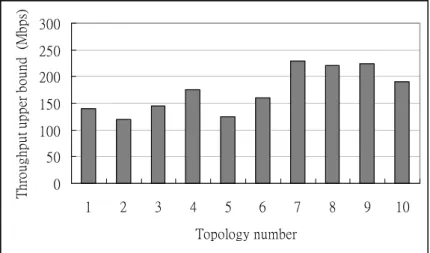
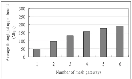
In this section, we consider a 8× grid network. For each topology, we 8 choose 30 mesh APs and 6 mesh gateways randomly. The remaining nodes are pure routers. Each pure router is equipped with 2 backhaul interfaces and each mesh gateway is equipped with 5 backhaul interfaces and each mesh AP is equipped with 2 backhaul interfaces and 1 client interface. The capacity of each channel is 10 Mbps and the capacity of wired link is 100 Mbps. We define the maximum flow of the network as the throughput upper bound. Figure 5.1 shows

the effects of different topologies on the throughput upper bound. In this figure, the largest throughput upper bound and the least throughput upper bound among these topologies are 230 Mbps and 120 Mbps, respectively. It shows that a better deployment of mesh routers is important. Figure 5.2 shows the effects of varying the number of mesh gateways on the average throughput upper bound. Note that each data point is the average over the 1000 topologies. The number of mesh gateways goes from 1 to 6 and the figure shows that the average throughput upper bound increases with the number of mesh gateways. It also shows that the average throughput upper bound only has 190.35 Mbps when there are 6 mesh gateways. That is because every mesh AP and every pure router are only equipped with 2 backhaul interfaces. Figure 5.3 shows the effects of varying the number of backhaul interfaces equipped at each mesh AP and each pure router on the average throughput upper bound. Note that each data point is the average over the 1000 topologies. The number of backhaul interfaces equipped at each mesh AP and each pure router goes from 2 to 5 and the figure shows the average throughput upper bound increases with the number of backhaul interfaces equipped at each mesh AP and each pure router. The average throughput upper bound can reach 281.145 Mbps when 5 backhaul interfaces equipped at each mesh AP and each pure router.

0 50 100 150 200 250 300 1 2 3 4 5 6 7 8 9 10 Topology number T hr oughput u ppe r bound ( M bps )

0 50 100 150 200 250 300 1 2 3 4 5 6 Number of mesh gateways

A ve ra ge thr ou ghput uppe r bound (M bps )

Figure 5.2: Throughput upper bound increases with the number of mesh gateways. Each data point is the average over the 1000 topologies.

0 50 100 150 200 250 300 2 3 4 5

Number of backhaul interfaces equipped at each mesh AP and each pure router

A ve ra ge thr oughput uppe r bound (M bps )

Figure 5.3: Throughput upper bound increases with the number of backhaul interfaces equipped at each mesh AP and each pure router. Each data point is the average over the 1000 topologies.

Chapter 6

Conclusion and Future Work

In this thesis, given the deployment of mesh routers and the number of radio interfaces of each mesh router, we want to find the maximum flow from mesh clients to the wired Internet under interference-free assumption. We define the maximum throughput of the problem as an upper bound of the throughput for the given wireless mesh network. The proposed problem is transformed into a maximum flow problem and then the problem can be solved by existing maximum flow algorithms. Therefore, an upper bound of the throughput for the given wireless mesh network can be obtained in polynomial time. The simulation results show that the upper bound of the throughput is affected by the deployment of mesh routers, the number of mesh routers which serve as gateway and the number of radio interfaces of each mesh router.

Note that the maximum flow of the resulting graph determines a set of routes which forms a subgraph. This subgraph preserves the maximum throughput for the wireless mesh network. In the future, we can consider a channel assignment problem for the wireless mesh networks based on the subgraph which is constructed by the resulting flow graph. If a feasible channel assignment is found, then this assignment is optimal for maximizing throughput.

References

 

 

[1] I.F. Akyildiz, X. Wang, and W. Wang, “Wireless mesh networks: a survey,” Elsevier Computer Networks, vol. 47, pp. 445-487, March 2005. [2] S. Avallone and I. F. Akylildiz, “A channel assignment algorithm for

multi-radio wireless mesh networks,” Computer Communications, vol. 31, pp. 1343-1353, May 2008.

[3] S. Avallone, I.F. Akyildiz and G. Ventre, “A Channel and Rate Assignment Algorithm and a Layer-2.5 Forwarding Paradigm for Multi-Radio Wireless Mesh Networks,” IEEE/ACM Transactions on

Networking, vol. 17, pp. 267-280, Feb. 2009.

[4] A. Raniwala, K. Gopalan, and T.C. Chiueh, “Centralized Channel Assignment and Routing Algorithms for Multi-Channel Wireless Mesh Networks,” ACM SIGMOBILE Mobile Computing and Communications

Review, vol. 8, pp. 50–65, April 2004.

[5] M. Kodialam, T. Nandagopal, “Characterizing the capacity region in multi-radio multi-channel wireless mesh networks,” Proceedings of the

11th annual international conference on Mobile computing and networking,

pp. 73–87, 2005.

[6] M. Alicherry , R. Bhatia , and L.E. Li, “Joint channel assignment and routing for throughput optimization in multi-radio wireless mesh networks,” Proceedings of the 11th annual international conference on

Mobile computing and networking, pp58-72, September 2005.

[7] J. Tang, G. Xue and W. Zhang, “End-to-end rate allocation in multi-radio wireless mesh networks cross-layer schemes,” Proceedings of the 3rd

international conference on Quality of service in heterogeneous wired/wireless networks, 2006

[8] A.H.M. Rad and V.W.S. Wong, “cross-layer fair bandwidth sharing for multi-channel wireless mesh networks,” IEEE Transactions on Wireless

Communications, vol. 7, pp. 3436-3445, September 2008.

Interface Assignment, Channel Allocation, and Routing for Multi-Channel Wireless Mesh Networks,” IEEE Transactions on Wireless

Communications, Volume: 6, pp. 4432-4440, December 2007.

[10] A. Raniwala and T. Chiueh, “Architecture and algorithms for an IEEE 802.11-based multi-channel wireless mesh network,” Proc. IEEE

INFOCOM, vol. 3, pp. 2223–2234, March 2005.

[11] H. Wu, F. Yang, K. Tan, J. Chen, Q. Zhang and Z. Zhang,“Distributed Channel Assignment and Routing in Multiradio Multichannel Multihop Wireless Networks,” IEEE Journal on Selected Areas in Communications, vol. 24, pp. 1972-1983, Nov. 2006.

[12] K. Jain, J. Padhye, V. N. Padmanabhan, and L. Qiu, “Impact of

interference on multi-hop wireless network performance,” Proceedings of

the 9th annual international conference on Mobile computing and networking, pp. 66–80, 2003.

[13] P. Gupta and P. R. Kumar, “The Capacity of Wireless Networks,” IEEE

Transactions on Information Theory, vol. 46, pp. 388-404, Mar 2000.

[14] R.K. Ahuja, T.L. Magnanti, and J.B. Orlin, “Network Flows: Theory Algorithms, and Applications,” Prentice-Hall, Englewood Cliffs, NJ, 1993. [15] L. R. Ford and D. R. Fulkerson, “Flows in Networks”, Princeton

University Press, 1962.

[16] J. Edmonds AND R.M. Karp, “Theoretical Improvements in Algorithmic Efficiency for Network Flow Problems,” Journal of the ACM (JACM), vol. 19, pp. 248-264, April 1972.

[17] E. A. Dinic, “Algorithm for solution of a problem of maximum flow in a network with power estimation,” Soviet Mathematics Doklady, 11(5): 1277–1280, 1970.

[18] “AMPL CPLEX.” http://www.ampl.com/DOWNLOADS/cplex80.html. [19] A. Lucena and J. E. Beasley, “Branch and cut algorithms,” in Advanced in

Linear and Integer Programming, J. E. Beasley, Ed. Oxford University Press, 1996.