行政院國家科學委員會補助專題研究計畫成果報告
※※※※※※※※※※※※※※※※※※※※※※※※※※※※※※※※※※※※ ※ ※ ※ ※ ※個 別 客 戶 忠 誠 度 之 衡 量 :
※ ※購買率層級式貝氏統計分析預測模式之建立
※ ※ ※ ※ ※ ※※※※※※※※※※※※※※※※※※※※※※※※※※※※※※※※※※※※計畫類別:
þ
個別型計畫 □整合型計畫
計畫編號:NSC 89-2416-H-002-055-
執行期間:88 年 8 月 1 日至 89 年 7 月 31 日
計畫主持人:任立中
共同主持人:
本成果報告包括以下應繳交之附件:
□赴國外出差或研習心得報告一份
□赴大陸地區出差或研習心得報告一份
þ出席國際學術會議心得報告及發表之論文各一份
□國際合作研究計畫國外研究報告書一份
執行單位:台灣大學國際企業學系
中 華 民 國 89 年 9 月 20 日
行政院國家科學委員會專題研究計畫成果報告
計畫編號:NSC 89-2416-H-002-055-
執行期限:88 年 8 月 1 日至 89 年 7 月 31 日
主持人:任立中 台灣大學國際企業學系
共同主持人:
計畫參與人員:周建亨 文化大學國際企業研究所
WESTERN DECISION SCIENCES INSTITUTE 20TH
ANNUAL MEETING
A Bayesian Appr oach to Estimating Expected Pur chase Fr equency
in Dir ect Mar keting
by
Lichung Jen
National Taiwan University Department of International Business
50, Lane 144, Sec. 4, Keelung Rd. Taipei, Taiwan
Chien-Heng Chou Chinese Culture University Department of Business Administration
55, Hwa Kang Rd. Hwa Kang, Yang Ming Shan
Taipei, Taiwan
and Greg M. Allenby Ohio State University
2100 Neil Avenue Columbus, OH 43210
April 18-22, 2000
Ritz Carlton Hotel at Kapalua, Island of Maui, Hawaii, USA
A Bayesian Appr oach to Estimating Expected Pur chase Fr equency
in Dir ect Mar keting
Abstract
Direct marketers are often faced with the task of ranking, or scoring individual customers in terms of their expected value to the firm. A critical element of these scoring systems is expected frequency of customer interaction. In this paper the authors develop a hierarchical Bayes model of purchase frequency that combines a Poisson likelihood with a gamma mixing distribution, where is mixing distribution is a function of covariates. The proposed model is evaluated with two direct marketing datasets, and is shown to provide improved estimates of purchase frequency, particularly for customers with short purchase histories or who have infrequent interaction with the firm.
A Bayesian Appr oach to Estimating Expected Pur chase Fr equency
in Dir ect Mar keting
1. Intr oduction
The frequency that a customer interacts with a firm is one of the most important indicators of their financial value. Customers who interact frequently are expected to generate a greater stream of revenue and often have a longer expected life than those who interact infrequently. In direct marketing, the frequency of interaction is an important component of customer scoring algorithms which are used to rank customers in terms of their overall value (see Stone 1994, David Shepard Associates 1995). However, estimates of expected purchase frequency are often very noisy because customer interactions do not follow regular patterns with fixed periods. Orders are often placed at irregular time intervals, and as a result simple estimates of expected frequency based on the number of orders placed during a prescribed period (e.g. the last three or six months) are sometimes unreliable.
In this paper we propose a hierarchical Bayes (HB) approach to estimating expected purchase frequency that are more reliable than simple estimates without placing undue restrictions on their variability. Model-based estimates of purchase frequency typically employ a Poisson distribution for the number of orders placed in a given time period. Heterogeneity in purchase frequency can be incorporated into the Poisson model by relating the intensity parameter (λ) to observed covariates. A drawback of this approach is that firms with equal covariate values (e.g. all large firms) are assumed to have the same purchase frequency.
Random-effect specifications avoid this problem by introducing unobserved heterogeneity into the model specification. The gamma distribution is often used as the random-effects distribution for the intensity parameter in a Poisson model, resulting in the well known negative binomial distribution (see Cameron and Trivedi 1986; Ehrenberg 1988; Morrison and Schmittlein 1988). While the negative binomial model allows for more flexible dispersion of the intensity parameter, it does not provide individual-level estimates of purchase frequency. Although covariates can be incorporated into the resulting negative binomial likelihood, this model suffers from the same problem as the
Poisson model – that is, it produces common estimates for units of analysis (e.g. customers) with equal covariate values.
We propose use of a hierarchical Bayes model of purchase frequency that combines a Poisson likelihood with a gamma distribution of heterogeneity. Our hierarchical Bayes model allows for dispersion in the intensity parameter similar to the negative binomial distribution while producing individual-level estimates of purchase frequency. Further, we show how to introduce covariates into the model specification that serve to shift the location of the random-effects distribution, thus facilitating prediction of purchase frequency for new customers who have a short purchase history, or possibly no history, with a firm.
In the next section we develop a hierarchical Bayes model and compare it to other commonly used methods of estimating purchase frequency. We then apply the model to direct marketing data and compare its performance to traditional methods, followed by some concluding remarks.
2. The Model
Direct marketers routinely collect information about the timing of customer purchases. In the case of business-to-business marketing, customers are individual firms who place orders through time. For consumer markets, customers are individual households that make frequent purchases from various product categories. The Poisson distribution is the simplest approach to modeling the number of purchases within a given time period. This model has been used in a wide variety of applications ranging from studying patent applications (Hausman, Hall and Griliches, 1984) and highway fatalities (Michener and Tighe, 1992) to non-durable purchases (Bucklin, Gupta and Siddarth, 1998). Denote yi as the number of times the i
th
customer interacts with the firm in a time period of length T, which is assumed to be Poisson distributed:
Pr(yi |λi,T) =
i
y iT)
where λi= E(yi)/T is the purchase frequency. Covariates can be introduced into this model
by relating them to the purchase rate through a log linear model: λi = exp(xi′β), where xi
denotes the vector of the ith
subject’s characteristic variables and β is the corresponding coefficient vector of xi. Without loss of generality, we suppress the notation for the time
period, T, in the following discussion and interpret λi as the expected number of customer
orders in a given period.
Although the Poisson regression likelihood offers a simple approach to modeling purchase frequency, the model is restrictive in that it assumes that the mean and variance of the data are equal. In practice, the variance of the data is often greater than the mean, resulting in inconsistent estimates of model parameters when the Poisson likelihood is used (Grogger and Carson 1991; Hausman, Hall and Griliches 1984; Shaw 1988). To accommodate this over-dispersion, a random-effects distribution for λi is assumed instead
of a log linear model. This assumption results in a model capable of reflecting data with greater variation. When the random-effects are assumed to be distributed gamma, the result is the negative binomial distribution (NBD) model.
NBD Model
The NBD model uses the gamma distribution to integrate out the individual λi’s,
resulting in a marginalized likelihood that is a function of the parameters of the gamma distribution (see Ehrenberg 1988, Morrison and Schmittlein 1988):
Pr(yi|α,θ) = θ θ θ θ α λ θ α λ λ + + + − =
∫
( | ) ( | , ) 1 1 11 i y i i i i i i y y d g y p (2)where g(λi|α,θ) is a gamma distribution, α is the shape parameter and θ is the location –
scale parameter. The expected value of λ is equal to αθ. The likelihood of the NBD model is defined as the product of the term on the left hand side over the i customers in the sample. Since Ehrenberg (1959) first introduced this model to marketing literature, it has been used in many studies ranging from predicting new product sales to modeling
inventory control (see Brockett, Golden, and Panjer 1996, Ehrenberg 1988, Massy, Montgomery, and Morrison 1970, Morrison and Schmittlein 1988). The focus of these studies is to describe the distribution of purchase frequencies in particular markets. That is, the NBD model yields estimates of α and θ which describe the distribution of λi, and do not
yield individual-level estimates of λi. This is a shortcoming of the NBD model.
In many direct marketing applications the focus of analysis is on the expected behavior of individual customers. Customers are frequently ranked according to the likelihood of response to a particular offering, or in terms of their expected contribution to the long-term profitability of the firm. Disaggregate estimates of expected purchase frequency for each customer is therefore desired. While it is possible to introduce covariates into the NBD likelihood in equation (2) (e.g. E[λi|α,θi] = αθi = exp(xi′β)) the
model suffers from the same problem identified with the Poisson likelihood. That is, customers with the same covariate values are assigned the same expected purchase frequency. This is so because the NBD model does not yield individual-level estimates of purchase frequency (λi), and the expected purchase frequency for a given vector of
covariates (E[λi|α,xi,β]) is used instead.
Hierarchical Bayes Model
The hierarchical Bayes model combines the Poisson likelihood with the gamma random-effects distribution without integrating out the individual λi’s. In contrast to
equation (2), the gamma distribution is viewed as part of the prior distribution to arrive at the posterior. In general notation, let Θ denote the parameters of a model. Then Bayes rule states that the posterior is proportional to the product of the prior and the likelihood:
π(Θ|Data) ∝ λ (Data|Θ) π(Θ) (3)
where λ denotes the likelihood, π(Θ) is the prior and π(Θ|Data) is the posterior. A Bayesian version of the NBD model then becomes:
where π(α) and π(θ) are prior distributions on the parameters of the gamma distribution, and the last three factors on the right side of the equation form the prior distribution. π(α) and π(θ) are typically specified to have minimal influence on the posterior distribution. Estimates of individual purchase frequency is obtained by integrating the joint posterior density:
π(λj|{yi}) =
∫ ∫
Λ π(α,θ,{λi}|{yi}) dα dθ dλ-j (5)where “-j” denotes “all units except j.”
The result is individual level estimates of purchase timing that reflect both the data from the individual customer (yj) and other customers as expresses through the
random-effects distribution. This combination of information results in individual estimates of purchase frequency that are less extreme than those based on the data alone (equation 2.1). In addition, covariates can be introduced into the model specification by relating them to parameters of the gamma distribution: θi = exp(xi′β).
The evaluation of the integral in (5) has previously been infeasible because of its high dimensions. However, recent advances in Markov chain Monte-Carlo estimation (e.g. Gibbs Sampling) now make this evaluation feasible. Combining the Poisson likelihood with gamma heterogeneity is a relatively straightforward task. The introduction of covariates, however, severely complicates the Markov chain. In the appendix we provide an estimation algorithm in where θ, the location parameter of the gamma distribution, is related to dummy-variable covariates through a link function θi = exp(xi′β).
Markov chain Monte-Carlo estimation is a simulation-based estimation procedure in which random draws are recursively simulated from the full conditional distributions of the model, and are used as conditioning arguments in subsequent draws. Upon convergence, these draws are from the true posterior distribution (Gelfand and Smith, 1990). Details of the computational algorithm are provided in the appendix. In the analysis presented in the next section, we estimate the model using 10,000 iterations of the Markov chain, from which the first 9500 iterations were discarded and the last 500 iterations were used to form
estimates of the posterior distribution of model parameters. Time series plot of the draws indicate that convergence of the chain from multiple initial values.
3. Empir ical Applications.
In this section we compare the in-sample and predictive fits of the hierarchical Bayes model to other methods of estimating expected purchase frequency with two datasets. The first dataset is from an office supply company engaged in business-to-business selling in the United States. The data span a period of three years, providing sufficiently long purchase histories to conduct predictive tests. The sample is comprised of 4795 firms that were randomly selected from company records. Covariates used in the analysis include the geographic region of the firm, the type of business, and the average purchase amount recorded in increments of $50 up to $200 and above. In total, there were ten dummy variables available for analysis (see table 1a). The average purchase frequency across all firms is equal to 4.51 per year.
A direct marketing company, located in Taiwan and specializing in cosmetics, shampoo, toothpaste and food supplements, provided the second dataset. In contrast to the first dataset, purchases are made by individual consumers and not other firms. The average purchase frequency is equal to 22.38 per year, allowing examination of the performance of the hierarchical Bayes model with longer purchase histories. This dataset also spans a three year period, and is comprised of 1725 customers randomly selected from company records. Covariates examined include the gender of the customer, geographic location and the average purchase amount recorded in increments of 5000 NT dollars up to 15,000 NT dollars (see table 1b). In total, there were eight dummy variables available for analysis in the second dataset.
Parameter estimates for the Poisson, NBD and hierarchical Bayes models are reported in tables 1a and 1b. The Poisson and NBD models were estimated by the method of maximum likelihood. Recall that for the Poisson model the intensity parameter, λ, is linked to the covariates through the log linear model λi = exp(xi′β), while for the NBD
model E[λi|α,θi] = exp(xi′β). In the hierarchical Bayes model it is more natural to relate θi,
the scale parameter of the gamma distribution, to the covariates through a log-linear model:
NBD models should agree with each other, but the intercept for the HB model will be different when α is different from one. This is true because in the gamma distribution E[λi|α,θi] = αθi = exp(ln(α) + x′β) implying that slope coefficient estimates should not be
affected.
Across both datasets we find close agreement in the coefficient estimates for the Poisson, NBD and hierarchical Bayes models. The over-dispersion afforded by the NBD and HB models does not lead to tangible differences in the point estimates. Furthermore, we note that the prior distributions used in the Bayesian model (equation 4) do not exert much influence on the posterior estimates relative to estimates based entirely on the likelihood. We conclude that the three models provide equivalent information about the distribution of purchase frequencies and their relationship to the covariates. The advantage of the hierarchical Bayes model, however, is its ability to generate individual-level estimates of purchase frequency.
[Tables 1a and 1b]
Tables 2a and 2b illustrate the difference in in-sample fit of the Poisson, NBD and hierarchical Bayes model. Twelve randomly selected customers (firms and individuals) were selected from each dataset. Customer identification numbers and associated covariates are display on the left side of the table. The observed number of purchases is reported in the center of the table, and the right side of the table contains various estimates of the customer’s expected purchase frequency. Table 2a reports results for the firm engaged in business-to-business marketing, while table 2b reports results for the firm selling consumer products.
The hierarchical Bayes estimates of purchase frequency more closely mirror the observed number of purchases than estimates from the Poisson and NBD models. As stated earlier, these models restrict the variation in the individual-level estimates so that customers with identical covariates have identical expected frequencies. Both the Poisson and NBD model estimates are close to the group mean, defined as the simple average of all purchases for firms with the same demographic variables. The group mean estimate is equivalent to what would be obtained by regressing the observed purchases on the covariates.
In addition to fitting the data better than traditional models, the hierarchical Bayes estimates are less extreme than the observed purchases. This tendency is common with
Bayesian estimates, and is due to the posterior estimates being derived from both the likelihood (the observed purchases) and the random-effects distribution (see equations 4 and 5). The random-effects distribution serves to shrink the individual estimates toward the average purchase frequency. In our application, the mean of the random-effects distribution is related to covariates, so the amount of shrinkage is dependent on the covariate values.
[Tables 2a and 2b]
Summary measures of the in-sample and predictive fit of the various models were calculated by re-estimating the model on a subset of the original data and by using the remainder as a holdout. Both the business-to-business and consumer direct marketing data sets span a total of three years. The first half of each customer’s purchase history (spanning 1.5 years) was used to assess the in-sample fit of the model, and the second half was used to assess out-of-sample fit.
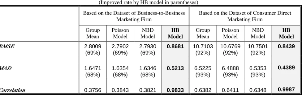
Table 3 reports the in-sample fit of various models used to estimate expected purchase frequency. Two measures of fit are reported, the root mean squared error (RMSE) and mean absolute deviation (MAD) between the fitted values and the observed frequency. Also reported is the correlation between the expected and observed frequencies. This later statistic can be used to assess the accuracy of an implied ranking of the firms based on expected purchase frequency. The results reported in table 3 is consistent with those reported in table 2, indicating that the hierarchical Bayes model produces individual estimates that much more closely mirrors the observed purchase frequencies.
[Table 3]
Table 4 reports out-of-sample fits of the models under various lengths of the customer’s purchase history. We use either the first 6, 12 or 18 months of records in the first half of the customer purchase history to produce estimates of expected purchase frequency, and then compare these estimate to observed frequencies in the second half of the data. We expect that with very limited customer purchase histories, the “group mean”, Poisson, NBD and hierarchical Bayes models to predict with similar accuracy. This is so because the parameter estimates reported in tables 1a and 1b are approximately equal. However, as the length of the purchase history increases from 6 to 18 months, the
hierarchical Bayes predictions will differ from the other models because of its ability to produce posterior estimates of purchase frequency that blend the aggregate level information contained in the hyper-parameters with an individual’s data.
The predictive performance of the Bayes model is slightly better than the aggregate models when there exists limited purchase histories (e.g. 6 months), slightly better than the individual model when there exists long purchase histories (e.g. 18 months), and substantially better than all models in other cases. In comparison to the individual model, which simply equates expected purchase frequency with the observed frequency, the hierarchical Bayes estimates are more accurate when there exists limited individual-level information. For the business-to-business dataset, which has relatively infrequent customer interactions, the HB estimates are 13% more accurate than the individual estimates when forecasts are based on 6 months of buying records. As the length of the purchase history increases, the individual and HB estimates converge, and offer substantial improvement relative to the group mean, Poisson and NBD models.
[Table 4]
The hierarchical Bayes model offers a compromise between an individual model that estimates purchase frequency for each customer in isolation of the others, and standard models (group mean, Poisson and NBD) that pool purchases across customers and relate them to covariates such as demographics. The hierarchical Bayes estimator retains the flexibility of the individual model and produces individual-level estimates without imposing undue restrictions on the variability of these estimates as encountered with the standard models. The HB estimator is a compromise between the other estimators, offering the same in-sample fit as the individual estimates and equivalent predictive fits as the standard models when there is no data available for the new customers. In addition, the HB estimates are shown to be better than either when there exists minimal purchase histories (e.g. 6 or 12 months). The hierarchical Bayes estimator therefore dominates the other estimator in the two datasets examined in this study.
This paper introduces a hierarchical Bayes model of purchase frequency with observed and unobserved components of heterogeneity. Unobserved heterogeneity is captured through a gamma distribution for purchase rates, while observed heterogeneity is introduced by allowing the location-scale parameter of the distribution to depend on covariates. We demonstrate the advantage of using hierarchical Bayes approach relative to the other approaches, and provide algorithms for estimating the model with the Gibbs sampler. The hierarchical Bayes models, when estimated with simulation-based methods such as the Gibbs sampler, are particularly well suited to the analysis of direct marketing problems because they yield individual-level estimates as a by-product of the estimation procedure.
We demonstrate the HB approach to estimating expected purchase frequency in two datasets. Based on these results we expect the proposed methodology to yield improved estimates of expected frequency relative to conventional approaches, particularly when there exists limited information about any particular customer. This is because the hierarchical Bayes estimator augments the limited information contained in the customer purchase history with information from the random-effects distribution.
There are a number of avenues for future work in this area. First, our assumption of exponential interpurchase times may not be appropriate in some direct marketing contexts and may need to be relaxed. The exponential model implies that a constant hazard rate which may be overly restrictive in many circumstances. However, violations of this assumption would require longer purchase histories than that present in the business-to-business direct marketing problem analyzed in this paper (see Allenby, Leone and Jen 1999 for a model of purchase timing spanning six years). Second, we allow the location-scale parameter of the inverse gamma distribution to be related to indicator (dummy) variables. While many covariates used to model observed heterogeneity are measured on a nominal scale, it would certainly be desirable to allow for the location-scale parameter to be directly related to continuous covariates such as age or income. Finally, we note that customer scoring systems in direct marketing also use variables such as the monetary amount of the purchase to estimate the total worth of their customers. Extending the model to include multivariate response variables (e.g. inter-purchase time, monetary amount) would therefor be a fruitful avenue for future research.
Appendix: The Gibbs Sampler for Hier ar chical Bayes Model of Pur chase Rate
Purchases yi during time period T are distributed Poisson with gamma heterogeneity:
likelihood: λ
(
Yi = yiλi,T)
∝λiyie−λiT (A1) mixing distribution: π λ α θ λ α θ α α λ θ ( , ) ( ) i i i i e i i = −1 −Γ where θi =exp(xi′β) (A2)
The Gibbs sampler recursively generates draws from the full conditional distributions of the model. Below we derive the conditional distributions for the Poisson-Gamma model. Estimation Algorithm
1. Gener ate λi, i=1,… N (one unit at a time)
[
]
− − −[
′]
+ − − +[
′]
− − ∝ ∝ 1 1 exp( ) 1 ) exp( 1 , , , , α β λ λ λα λ β λ α λ β λ π i i i i i i i x T y i x i T y i i i iy T x e e eConsequently, λiis generated from a gamma distribution, G(A,B), where
α + =Yi A , and
[
]
1 1 ) exp( − − + ′ = T xi β B for i=1,...,N.2. Gener ate βk, k=1,… ,K (one coefficient at a time)
The posterior distribution of βk, given the other parameters, is
π β λ α( k{ }, ,i ik, ) (λ α βi , k, ik, ) (π βk) i N x T ∝ x T = ∏λ 1
In order to generate βk, we first re-parameterize βk by letting e k
k
β =ϕ and then derive the
posterior distribution of ϕk. We also assume that all the covariates xk, where k∈(1,Κ,K),
are 0-1 dummy variables. Since
ex e e x x j K jx j K i ij j j K j ij ij ' ( ) β = ∑= β = β = ϕ = = ∏ ∏ 1 1 1
The equation can be rewritten as
∏ − = − = ⋅ Γ = ′ ∏ K j ij x j i ij e x K j x j i i i 1 1 1 ) ( )) exp( , ( ϕ λ α α ϕ α λ β α λ π
Define xik N i N k = ∑ = 1 , S(k)={ xik |xik=1, i=1,… ,N}, and ∏ ≠ = = K k j j x j k i ij D 1 ) ( ϕ .
The likelihood of βk in terms of ϕk is
λ(ϕk i,λi, ) ϕ αx ϕ α Λ ϕ α Λ ϕ α i N x i N k x i N K x i N x T ∝ i i ik iK × − = − = − = − = ∏ 1 ∏ ∏ ∏ 1 1 2 1 1 1 2 exp−
(
⋅ ⋅)
− − − − = ∑ϕ1 ϕ2 ϕ ϕ λ 1 1 2 x x k x K x i i N i i Λ ikΛ iK ∝ ∑ ⋅ −( )
+( )
− − − ∈ − ∉ = ∑ ∑ ϕkα x ϕk λi i λ k i S i i k i S ik i N k k D D 1 1 1 1 exp ( ) ( ) ( ) ( ) ∝ ⋅ −( )
− − − ∈∑ ϕkαN ϕ λ k i i k i S k k D exp ( ) ( ) 1 1If the prior distribution of ϕk is Inverse Gamma distribution, IG(ak0, bk0), the conditional
posterior of ϕk is proportional to
( )
π ϕ λ( , , ( ), , , ) ϕ (α )exp ϕ λ ( ) ( ) k i ik i k k k k N a k k i i k i S x D a b T k k b D k 0 0 1 1 10 1 0 ∝ − + − + + − − ∈ − ∑ .then generate ϕk from Inverse Gamma αNk ak bk λi
( )
Diki Sk + + − − ∈ − ∑ 0 01 1 1 , ( ) ( ) 3. Gener ate α
The posterior distribution of α , given the other parameters, is
π α λ β( { },i k, ik, ) (λ α θ π αi , i) ( ) i N x T ∝ = ∏λ 1
Based on the equation (2), the likelihood of α is :
(
)
( )
( )
λα λ θ λ α θ λ θ α λ α α λ θ α λ θ i i i i i N i i i i N T e e i i i i , , ∝ = − − = − = ∏ 1 ∏ 1Γ 1ΓIf the prior distribution of α is Uniform (M), then the posterior distribution of α, given λi and θi, is proportional to ∏ = N i i i poisson continuous 1 θ λ
which is the product of N continuous Poisson distributions.
REFERENCES
Allenby, Greg M., Robert P. Leone and Lichung Jen (1999) “A Dynamic Model of Purchase Timing with Application to Direct Marketing,”Journal of the American Statistical Association, forthcoming.
Brockett, Patrick L., Linda L. Golden, and Harry H. Panjer (1996), “Flexible Purchase Frequency Modeling,”Journal of Marketing Research, 33 (February), 94-107. Bucklin, Randolph E., Sunil Gupta, and S. Siddarth (1998), “Determining Segmentation
in Sales Response Across Consumer Purchase Behaviors,”Journal of Marketing Research, 35 (May), 189-97.
Cameron, A. Colin and Pravin K. Trivedi (1986), “Econometric Models Based on Count Data: Comparisons and Applications of Some Estimators and Tests,”Journal of Applied Econometrics, 1, 29-53.
David Shepard Associates, Inc. (1995), The New Direct Marketing: How to Implement a Profit-Driven Database Marketing Strategy, New York: Richard D. Irwin, Inc. Ehrenberg, A. S. C. (1959), “The Pattern of Consumer Purchases,”Applied Statistics, 8
(1), 26-41.
---(1988), Repeat Buying, 2nd
ed., New York: Oxford University Press.
Gelfand, A. E. and A. F. M. Smith (1990), "Sampling-Based Approaches to Calculating Marginal Densities," Journal of the American Statistical Association, 85, 398-409. Grogger, J. T. and Richard. T. Carson (1991), “Models For Truncated Counts,”Journal of
Applied Econometrics, 6 (3), 225-38.
Hausman, Jerry A., Bronwyn. Hall, and Zvi. Griliches, (1984) "Econometric Models for Count Data With an Application to the Patents-R&D Relationship," Econometrica, 52 (4), 909-38.
Massy, William F., David B. Montgomery, and Donald G. Morrison (1970), Stochastic Models of Buying Behavior, Cambridge, MA: The MIT Press.
Michener, R. and C. Tighe (1992), "A Poisson Regression Model of Highway Fatalities," Externalities, American Economic Review, 82 (May), 452-56.
Morrison, Donald G. and David C. Schmittlein (1988), “Generalizing the NBD Model for Customer Purchases: What Are the Implications and Is It Worth the Effort?”
Shaw, D. (1988), “On-Site Samples’ Regression: Problems of Non-Negative Integers, Truncation, and Endogenous Stratification,”Journal of Econometrics, 37 (February), 211-23.
TABLE 1a
Poisson, NBD, and Hierarchical Bayes Parameter Estimates for Purchase Frequency (Based on the Dataset of Business-to-Business Marketing Firm)
Poisson Model NBD Model HB model
Parameters: Intercept 1.1775850 (0.030287) 1.1714120 (0.044671) 0.7421252 (0.0469742) Northeast -0.0473115 (0.017344) -0.0434026 (0.024860) -0.0439138 (0.0288897) Midwest -0.0461124 (0.021599) -0.0360934 (0.034944) -0.0362610 (0.0399340) South -0.0836994 (0.019296) -0.0906082 (0.028604) -0.0903015 (0.0354891) Insurance-related Firms 0.1550857 (0.071291) 0.1345827 (0.126180) 0.0820847 (0.1226750) Medical Offices 0.4716371 (0.034259) 0.4673243 (0.055080) 0.4103141 (0.0726537) Attorneys 0.3074149 (0.029032) 0.3134243 (0.058330) 0.2921774 (0.0625478) M1a 0.1811062 (0.034122) 0.1980594 (0.044355) 0.1478682 (0.0456894) M2b 0.4416289 (0.029336) 0.4453912 (0.042118) 0.3926779 (0.0335346) M3c 0.3266383 (0.031110) 0.3263928 (0.045612) 0.2724078 (0.0383798) M4d 0.2807466 (0.036344) 0.2927877 (0.046209) 0.2376187 (0.0530984) α 1.6192307 (0.017367) 1.618966 (0.035522) a
M1 dummy variable means average purchase amount less than 50 dollars.
b
M2 dummy variable means average purchase amount less than 100 dollars.
c
M3 dummy variable means average purchase amount less than 150 dollars.
d
M4 dummy variable means average purchase amount less than 200 dollars.
e
TABLE 1b
Poisson, NBD, and Hierarchical Bayes Parameter Estimates for Purchase Frequency (Based on the Dataset of Consumer Direct Marketing Firm)
Poisson Model NBD Model HB model
Parameters: Intercept 3.1740350 (0.013552) 3.1718070 (0.063229) 3.1787885 (0.0579631) Sex -0.0564288 (0.010285) -0.0326018 (0.046062) -0.0258470 (0.0454367) Area1 -0.0139500 (0.015485) -0.0841114 (0.072142) -0.0650743 (0.0692164) Area2 -0.0105712 (0.017424) -0.04119727 (0.086384) -0.0313596 (0.0789550) Area3 -0.0034828 (0.012585) 0.0110694 (0.054018) 0.0092028 (0.0584529) Area4 -0.2327633 (0.027680) -0.2136312 (0.136300) -0.1687566 (0.1096664) M1a -0.8596766 (0.019210) -0.8597417 (0.071179) -0.7633183 (0.0619591) M2b 0.0989403 (0.013993) 0.0967286 (0.066687) 0.1261607 (0.0568964) M3c 0.3855048 (0.015336) 0.3908373 (0.089264) 0.4012189 (0.0768399) α 0.9550396 (0.043521) 0.951763 (0.030209) a
M1 dummy variable means average purchase amount less than 5,000 NT dollars.
b
M2 dummy variable means average purchase amount less than 10,000 NT dollars.
c
M3 dummy variable means average purchase amount less than 15,000 NT dollars.
d
TABLE 2a
Comparison of Individual Purchase Frequency Estimates (Based on the Dataset of Business-to-Business Marketing Firm)
Covariates Expected Purchase Frequency
Group Customer No. Location Business Type Average Purchase Amount Observed Purchase Frequency Group Mean Poisson NBD HB 3808 West Attorneys M1 2 5.4616 5.2915 5.3811 2.7385 4256 West Attorneys M1 6 5.4616 5.2915 5.3811 5.7032 1 4291 West Attorneys M1 15 5.4616 5.2915 5.3811 12.7387 1564 South Insurance M2 1 5.3988 5.4227 5.2634 1.9991 2063 South Insurance M2 7 5.3988 5.4227 5.2634 6.4893 2 2297 South Insurance M2 26 5.3988 5.4227 5.2634 20.8529 2690 Midwest Medical M3 3 6.8040 6.8878 6.8829 3.7210 2706 Midwest Medical M3 7 6.8040 6.8878 6.8829 6.7339 3 3213 Midwest Medical M3 22 6.8040 6.8878 6.8829 18.9612 750 Northeast Others M4 3 4.0905 4.1001 4.1404 3.2876 1797 Northeast Others M4 16 4.0905 4.1001 4.1404 12.4753 4 475 Northeast Others M4 61 4.0905 4.1001 4.1404 44.6723 TABLE 2b
Comparison of Individual Purchase Frequency Estimates (Based on the Dataset of Consumer Direct Marketing Firm)
Covariates Expected Purchase Frequency
Group
Customer
No. Gender Location
Average Purchase Amount
Observed Purchase
Frequency GroupMean
Poisson NBD HB 1723 Male North M1 1 8.9775 9.4308 8.9832 1.7995 1505 Male North M1 9 8.9775 9.4308 8.9832 8.8012 1 475 Male North M1 27 8.9775 9.4308 8.9832 25.4276 175 Female Central M2 25 25.994 26.112 25.212 25.3418 297 Female Central M2 95 25.994 26.112 25.212 92.8335 2 320 Female Central M2 9 25.994 26.112 25.212 9.5047 1628 Male South M3 7 33.381 33.103 34.505 7.6979 1349 Male South M3 28 33.381 33.103 34.505 27.7139 3 1282 Male South M3 37 33.381 33.103 34.505 36.7944 777 Female East M1 32 5.9655 8.0172 8.1534 32.0145 437 Female East M1 20 5.9655 8.0172 8.1534 18.9749 4 1355 Female East M1 6 5.9655 8.0172 8.1534 6.0578
TABLE 3 In-Sample Fit
(Improved rate by HB model in parentheses) Based on the Dataset of Business-to-Business
Marketing Firm
Based on the Dataset of Consumer Direct Marketing Firm Group Mean Poisson Model NBD Model HB Model Group Mean Poisson Model NBD Model HB Model RMSE 2.8009 (69%) 2.7902 (69%) 2.7930 (69%) 0.8681 10.7103 (92%) 10.6769 (92%) 10.7501 (92%) 0.8439 MAD 1.6471 (68%) 1.6354 (68%) 1.6346 (68%) 0.5213 6.5225 (93%) 6.4888 (93%) 6.5353 (93%) 0.4389 Correlation 0.3756 0.3843 0.3821 0.9833 0.6382 0.6411 0.6348 0.9987
TABLE 4
Predictive Performance Based on Different Amount of Information (Improved rate by HB model in parentheses)
Based on the Dataset of Business-to-Business Marketing Firm
Based on the Dataset of Consumer Direct Marketing Firm Individual Model Group Mean Poisson Model NBD Model HB Model Individual Model Group Mean Poisson Model NBD Model HB Model RMSE
1. Based on 6 months buying records 4.3284
(13%) 3.9148 (4%) 3.9183 (4%) 3.9188 (4%) 3.7640 17.4180 (4%) 17.1273 (2%) 17.1429 (2%) 17.3474 (3%) 16.7722
2. Based on 12 months buying records 3.8349
(9%) 3.7162 (6%) 3.7152 (6%) 3.7136 (6%) 3.4848 15.8343 (2%) 16.4412 (5%) 16.4154 (5%) 16.5565 (6%) 15.5510
3. Based on 18 months buying records 3.2134
(2%) 3.6397 (13%) 3.6354 (13%) 3.6340 (13%) 3.1515 14.0963 (1%) 15.6934 (11%) 15.6741 (11%) 15.6934 (11%) 13.9247 MAD
1. Based on 6 months buying records 2.4795
(24%) 2.0360 (8%) 2.0176 (7%) 2.0181 (7%) 1.8812 11.5536 (6%) 11.5652 (6%) 11.4773 (6%) 11.6489 (7%) 10.8358
2. Based on 12 months buying records 1.9572
(16%) 1.8514 (11%) 1.8297 (10%) 1.8261 (10%) 1.6390 10.5035 (3%) 11.1601 (9%) 11.0827 (8%) 11.2290 (9%) 10.1634
3. Based on 18 months buying records 1.5827
(9%) 1.7476 (17%) 1.7214 (16%) 1.7159 (16%) 1.4470 9.2493 (2%) 10.5432 (14%) 10.4779 (14%) 10.5073 (14%) 9.0310