行政院國家科學委員會專題研究計畫 期中進度報告
虛擬實境之多媒體影音控制技術開發(2/3)
計畫類別: 個別型計畫
計畫編號: NSC92-2213-E-009-053-
執行期間: 92 年 08 月 01 日至 93 年 07 月 31 日
執行單位: 國立交通大學電機與控制工程學系
計畫主持人: 林進燈
報告類型: 精簡報告
報告附件: 出席國際會議研究心得報告及發表論文
處理方式: 本計畫可公開查詢
中 華 民 國 93 年 5 月 7 日
虛擬實境之多媒體影音控制技術開發
(2/3)
計畫編號:NSC-92-2213-E-009-053-
執行期限:
92.8.1-93.7.31
主持人:林進燈 國立交通大學 教授
執行機構:國立交通大學電機與控制工程研究所
一、前言
本計畫為「虛擬實境之多媒體影音控
制技術開發」,研發重點在於結合各種
電機資訊與人工智慧等科技,讓虛擬實
境系統具備有智慧型的反應能力,研究
的方向有虛擬實境多媒體系統的影像控
制、音訊控制與通訊等三項技術的開發
與研究。在本期的計畫中,除了已就音
訊控制技術開發的部份,包括「不特定
語者語音辨識系統核心辨識器」與「環
場音效系統之研究」做研究外,這裡將
再針對3D音場技術作探討;此外,就影
像控制技術開發的部分,我們也說明關
於三維立體影像重建之研究。
關於3D音場技術部份,我們嘗試建立
3D環繞音效的系統模型,主要技術包括
以PCA對已有的頭部相關位置脈衝響應
(Heade-Related-Impulse-Response,HRIR)
資料庫作分析及壓縮,同時利用類神經
網路內插的特性將空間中任一位置的
HRIR合成出來,以達成3D音場之重建與
模擬。在三維立體影像重建之研究中,
我們提出一個以類神經網路為基礎的適
應性整合式反射模型。這個類神經網路
自動整合光學成像上的散射與反射成
分,使得我們可以個別考慮物體表面上
每一點的成像特性,並且針對表面不同
反射率的問題加以處理。
以下將分別針對此二主題進行說明。
二、3D 音場技術之研究
AbstractIn this project, we build a virtual 3D environment. We use the MIT head-related impulse responses (HRIRs) as our database. More specifically, it deals with synthesis of 3D moving sound to be supplied binaurally through headphones. Then, we propose an efficient method, which can reduce the
information size and interpolate the nonsampling HRIR while retaining high resolution of localization. First, in this model the HRIRs are expressed as weighted combinations of a set of eigentransfer functions. The weights applied to each eigentransfer functions only of spatial location and are thus termed SCFs (Spatial Characteristic Functions).
The SCFs that we extract, however, are restricted to the specified azimuths and elevations that the HRIR database records. The SCFs for the nonsample spatial location are unknown. So we use the architecture of radial basis function network (RBFN) with Von Mises function as activation functions for classification of the spatial characteristic features. This neural network is called VMBFN (Von Mises Basis Functions Network). The VMBFN used here can solve the problem of approximation and interpolation. When using the orthogonal least square learning algorithm to train VMBFN, the RMSE (Root Mean Square Error) is
minimal. Through convolution the source sound with
the simulated HRIR, we can synthesize the spatial sound over headphone..
1. Introduction
Sound is an extremely useful medium for conveying information. We are focused on study of the head-related impulse responses (HRIRs). In this case, the direction of arrival of the sound can be controlled by filtering the original monaural signal through a proper set of previously measured HRIRs But the database needs a lot of memories to record. It is difficult to allocate such a large memories on the IC. The present work addresses the problem of spatial sound generation at a reduced storage cost. So we propose a neural network model of binaural hearing based on spatial feature extraction of the HRIRs.
As a consequence, estimating the HRIR associated with any desired source location asks for some interpolation scheme. When realizing moving sound, especial care must be taken to avoid audible discontinuities along the required path. So we also concentrate on the issue of the interpolation of HRIRs. Our neural network associated with spatial characteristic functions parameterized by angular positions provides proper localization for each sound source. Given the desired angles, only the corresponding spatial characteristic functions need to be computed. Therefore, this method can be more efficient than conventional HRIRs interpolation when dealing with multi-source synthesis. Furthermore, the method implicitly performs the spatial interpolation of the non-measured HRIRs.
In this project we propose an efficient method, which can reduce the information size and computation while retaining high resolution of localization. First, in this model the HRIRs are expressed as weighted combinations of a set of eigentransfer functions. The weights applied to each eigentransfer functions only of spatial location and are thus termed spatial characteristic functions. Then, we use the architecture of radial basis function network (RBFN) with Von Mises function as activation functions for classification of the spatial characteristic features. This neural network is called VMBFN. The VMBFN used here can solve the problem of approximation and interpolation. Through convolution the source sound with HRIR, we can synthesize the spatial sound over headphone. So we can build a virtual 3D environment.
2. Spatial Feature Extraction
The HMM, which uses probabilistic functions of Markov chains to model random processes, is a model of stochastic process. The effectiveness of this model class lies in its ability to deal with non-stationarity that often appears in the observed data sequences. HMMs usually turn out to be a good model for non-stationary process, such as the sequence of the speech observation vectors.
2.1 Basic Framework
Our goal in this chapter is to reduce the storage for HRIR through the dimension reduction of the data set. We use structural composition and decomposition of the database to compress the database. HRIRs of Kemar are our database. There were 710 measurements taken around the manikin at elevations
ranging from -40 to +90 at one meter in distance. ∘ ∘
Let hj denote the HRIR of location (θj, φj), where the
variable θ and φ correspond to any sample direction in azimuth and elevation, with j=1,2,…P, and P=710. hj is an 128×1 valued vector representing the 128 samples of the HRIR measured at the jth location.
A given normalized HRIR hj is decomposited by
bias i M i ij bias j j Qw h w q h h = + =
∑
+ =1 To reduce the amount of storage of HRIR we only record both the transformation matrix] , ,
[q1 q2 qM
Q= L and
w
j to replace record thedatabase of HRIRs. To accomplish this, we require an optimal linear dimension reduction technique. The method called principal component analysis is employed to get orthonormal transformation Q and the
corresponding
w
j.2.2 Principle Component Analysis
The PCA is used here to express the HRIRs in terms of an orthogonal function expansion. In our application, we derived orthonormal basis functions
from the normalized HRIRs. Let hj denote the HRIR
of location (θj, φj),with j=1,2,…P, and P=710. hj is an
128×1 valued vector representing the 128 samples of the HRIR measured at the jth location. Prior to deriving the basis function, the space sample average was subtracted from each normalized HRIR to remove the direction-independent component. The space
sample average is defined as
(
)
∑
= = P j j j av P h h 1 , 1 θ φis the sample mean and a time autocovariance matrix is then calculated by
(
)
[
]
[
(
)
]
T av j j P j av j j h h h h h P R =∑
− × − = ϕ θ ϕ θ , , 1 1 wh ich is a real valued matrix. The normalized HRIR, which corresponds to P=710 measured samples, areused to determine the
R
h. The eigenvectors of thecovariance matrix
R
h define the unit vectors vlrepresenting the orthogonal directions along which the
variance probes ψ(vl) (i.e., a function of variance)
have their extreme values, for l = 1, 2, … , N, N=128.
The eigenvalues {λ1, λ2, … , λN} define the extreme
values of the variance probes ψ(vl), where
R
hvl = λlvl,for l = 1, 2, … , N and the eigenvalues of
R
h bearranged in decreasing order λ1≥λ2≥...≥λN. This is an application of PCA to dimensionality reduction.
The eigenvectors of Rh are chosen as the
columns of an orthonormal transformation
matrix Q=[q1,q2,LqM] . Applying the PCA
methodology to this 128-dimenional representation for the spatially sampled HRIR, hj can be expressed by the
eigentransfer basis functions
q
i,
i
=
1
,...,
M
. Agiven normalized HRIR hj is represented by
av i M i ij av j j Qw h w q h h = + =
∑
+ =1 Next, we do an experiment for selection of eigenvectors. The eigenvectors of the covariance matrix corresponding to the largest eignvalues are often referred to as principal components in the context of statistical data analysis. The eigenvalues λi ,i=1,…,N represent the sample variance of
(
)
[
h
θ
j,
ϕ
j−
q
0]
, j=1,2,…,P projected onto eacheigentransfer function qi, i=1,…N. That is, the value o
f λi indicates the variability of projection of the data on the corresponding eigentransfer function. Hence, the number of eigenvectors, M, required to achieve a given mean squared error is determined by the relative size of the eigenvalues. The results below indicate that a very percentage of variability in the measured HRIR is represented using a relatively small value of M. Finally we choose M=14 as the number of eigenvectors.
Figure 2.1 Percent of variance as a function of M for Kemar Database 2 4 6 8 10 12 14 16 18 20 30 40 50 60 70 80 90 100 Numbers of M % va r(M )
2.3 Spatial Characteristic Functions The normalized HRIRs, which contain the spectral cues, are expressed as weighted combinations of a set of basis functions. The basis functions are real-valued eigenvectors that are derived from a covariance matrix of the measured HRIRs. The weights applied to each basis function and termed real spatial characteristic functions, define the relative contribution of each basis function to the HRIR and are real-valued functions of the spatial location. Samples of the M SCF at the P measurement locations are obtained from the M eigentransfer functions as
(
)
q[
h(
)
q]
i M j P w H j j i j j iθ ,ϕ = θ ,ϕ − 0, =1,2,..., ; =1,2,..., The eigentransfer functions
q
i,
i
=
0
,
1
,...,
M
onlycontain the temporal information of the HRIR and the
weight vectors
w
i,
i
=
1
,
2
,...,
M
are the spatialcharacter functions (SCF).
Although the HRIRs are the function of both space and time, we can separate the spatial characteristic features from the temporal features through spatial feature extraction. Because the sampling in space is more problematic than sampling in frequency because the spatial bandwidth is unknown, the required spatial sampling density and mathematics for reconstructing the HRIR as a continuous function of θ and φ from samples are unknown. So we don’t know the SCF of HRIR at an arbitrary spatial location that doesn’t sample in the database. The estimates of the SCF applied to each basis function can be obtained by interpolation. We will use neural network to solve the problem of interpolation.
3. Von Mises Basis Function Network The spatial characteristic functions that we extract, however, are restricted to the specified azimuths and elevations that the HRIR database records. The SCFs for the nonsample spatial location are unknown. We need a method to estimates of the spatial characteristic functions using the interpolate method at arbitrary spatial locations. So it is a problem of interpolation. There is a network proposed to solve the two problems of approximation and interpolation. The architecture of the network is similar to radial basis function network.
3.1 Von Mises Function
The Von Mises function is based on a spherical probability density function that was used to model line directions distributed with rotational symmetry. The expression for the Von Mises function, dropping the constant of proportionality and elevational weighting factor from the probability density function, is
( )
[ ( ) ][
π]
β φ[ ]
π θ α φ θ κ φ β θ α φ β 0, , 2 , 0 ,, sin sin cos cos cos 1
∈ ∈
= − + −
e
VMBF
where the variable θ and φ correspond to any sample direction in azimuth and elevation. For each Von Mises function, the parameters α and β correspond to a centroid in azimuth and elevation, and the parameter κ corresponds to a concentration parameter. Applications of the Von Mises function require an azimuthal range
in radians from 0 to 2π and elevational range form 0 toπ. Any sample direction (θ and φ) on the sphere will induce an output from a Von Mises function proportional to the angle between the sample direction and the centroid of the Von Mises function (α and β). The azimuthal periodicity of the basis function is driven by the cos(θ-α) term, which will be maximal when θ=α. The (sinφsinβ) term modulates the azimuthal term in the elevational plane, hence the requirement that φ range from 0 to π. As the sample elevation or the centroid elevation approaches either pole (0 or π), the multiplicative effect of (sinφsinβ) progressively eliminates the contribution of azimuthal variation and the (cosφcosβ) term dominates. The concentration parameter κ controls the function’s shape, where the larger the value the narrower the function width after transformation by the expansive exponential function. Although other spherical functions have been proposed for approximation on the sphere (e.g., thin-plate pseudo-spline), the VMBF serves as a convenient spherical analog of the well-known multidimensional Gaussian on plane. It resembles a bump on a sphere and behaves in a similar fashion to the planar Gaussian with the centroid
corresponding to the mean and κ-1 corresponding to
the SD. It differs from the thin-plate spline in that it has a parameter for controlling the width or concentration of the basis function, which allows the VMBF to focus resolution where needed. A mixture of Gaussians or Gabor functions has been used to model curve on the plane, so can a mixture of Von Mises functions. The parametersα, β and κ for a fixed number of basis functions are “learned” adaptively with a sum-of-squared-error cost function.
We transform the spatial characteristic functions from the Cartesian coordinate to polar coordinate. The shape of spatial characteristic functions in polar coordinate likes the combinations of Von Mises functions. So the spatial characteristic functions can be linear combined with many Von Mises functions. 3.2 Von Mises Basis Function Network
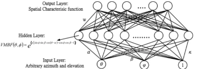
The construction of a Von Mises basis function network (VMBFN) in its most basic form involves three entirely different layers. The input layer is made up of source nodes (sensory units). The second layer is a hidden layer of high enough dimension, which the Von Mises basis function serves as the activation function to conforming to the RBF architecture as shown in Figure 3.1. The transformation from the input space to the hidden-unit space is nonlinear, whereas the transformation from the hidden-unit space to the output space is linear. Hence the reason for making the dimension of the hidden-unit space in an RBFN high. Through careful design, however, it is possible to reduce the dimension of the hidden-unit space, especially if the centers of the hidden units are made adaptive.
The input layer of each network consists of the any location in azimuth and elevation. The input requires an azimuthal range in radians from 0 to 2π and elevational range from 0 to π. The size of the hidden layer is determined as following section. For all experiments, the output layer of each network
consists of 14 nodes, each representing a spatial feature extraction.
Figure 3.1 The architecture of the Von Mises basis function network
3.3 Back Propagation Learning Algorithm for VMBFN
Over the course of iterative training, the centroid(α,β) of each basis function will move on the surface of the sphere, and the concentration κ of the basis function will change progressively. The learning algorithm used here is as follows.
(
n
+
1
)
=
Ω
(
)
+
( )
∆Ω
+
[
Ω
( )
−
Ω
(
−
1
)
]
Ω
n
η
n
µ
n
n
where
Ω
=
[
wt
T,
α
T,
β
T,
κ
T]
The first step in the development of such a VMBFN learning procedure is to define the instantaneous error measure for the pth data pair is defined by
(
)
2 , , , 2 1 p i p i p i t x E = −where
t
i,pis the desire output,x
i,p is the output of VMBFN. The derivative of the above instantaneous error measure with respect to the linear weights is written as( )
[
i i]
(
j j j)
i p t y VMBF w E κ β α φ θ φ θ, , , , , − = ∂ ∂ The derivative of the above instantaneous error measure with respect to the centroid αweights is
(
)
[
]
[
( )
]
(
j j j)
N i i i ij j j j j p VMBF wt y t E κ β α φ θ φ θ α θ β φ κ α , , , , , sin sin sin − ×∑
− × , × = ∂ ∂The derivative of the above instantaneous error measure with respect to the centroid β is
(
)
[
]
( )
[
]
(
j j j)
N i j i i i j j j j j p VMBF wt y t E κ β α φ θ φ θ β φ α θ β φ κ β , , , , , sin cos cos cos sin ,∑
− × × × − − = ∂ ∂ The derivative of the above instantaneous error measure with respect to the concentration κ is
(
)
[
]
( )
[
]
(
j j j)
N i j i i i j j j j j p VMBF wt y t E κ β α φ θ φ θ β φ α θ β φ κ κ , , , , , cos cos cos sin sin ,∑
− × × × + − = ∂ ∂3.4 Orthogonal Least Square Learning Algorithm for VMBFN
For VMBFN with a scalar output, an intelligent learning algorithm has been derived based on the orthogonal least squares method, which constructs VMBFN in a rational way. The algorithm chooses appropriate VMBFN centers one by one from training data points until a satisfactory network is obtained. Each selected centre maximizes the increment to
explained variance of the desired output, and so learning does not suffer numerical ill-conditioning problems. The main attraction of this algorithm is that it can naturally be implemented in a recursive form.
The orthogonal least square algorithm is a structural identification algorithm, and it constructs an adequate network structure in an intelligent way during learning. The task of network learning is to
choose appropriate centres cj and to determine the
corresponding weights θji, based on a given set of
network training inputs To avoid nonlinear learning, the VMBFN centres are to be selected from training data, and this is equivalent to a problem of subset model selection. The full model is defined by considering all the training data as candidates for centres.
Assume that a nonlinearity φ( ) is chosen and a
fixed width σ is given. A candidate centre
c
j=
x
( )
k
gives rise to a candidate hidden node φj in the full
VMBFN network of N hidden nodes. The desired outputs can be expressed as
( )
( )
i( )
o j ji j i t t e t i n d =∑
+ ≤ ≤ = 1 1 θ ϕwhere ei(t) are the errors between the desired outputs and the network outputs. The model in equation above is a linear regression model. φj(t) are known as the regressors, which are some fixed functions of the input vector x(t). By defining
( )
( )
[
]
o T i i i d d N i n d = 1 L 1≤ ≤( )
( )
[
]
o T i i i e e N i n e = 1 L 1≤ ≤( )
( )
[
N]
T j N j j ji = ≤ ≤ Φϕ
1Lϕ
1then for 1≤t≤N, equation above can collectively written as [ ] [ ] [ no] Nno N no N no i d e e d L L M O M L L L 1 1 1 11 1 + Φ Φ = θ θ θ θ or,
more concisely, in the matrix form
E
D=ΦΘ+
The parameter matrix Θ can readily be solved using
the LS principle.
Form a geometric viewpoint, the regressors Φj
form a set of basis vectors. These basis, however, are generally correlated. An orthogonal transformation can
be performed to transfer from the set of Φj into a set of
orthogonal basis vectors. This can be achieved by decomposing Φ into
Φ=WA
where A is an M×M triangular matrix with 1’s on the diagonal and 0’s below the diagonal.
The space spanned by the set of wj is the same
space spanned by the set of Φj, and equation
E
D=ΦΘ+ can be rewritten as
E WG
D= + The orthogonal least square solution is given by
= Nno N no g g g g G L M O M L 1 1 11 and
the ordinary LS solution Θ satisfy the triangular
system
G
AΘ=
Input Layer: Arbitrary azimuth and elevation Hidden Layer:
( ), [sinsincos( )coscos 1] e VMBFθφ= κ φ β θ−α+ φ β− .... ... θ φ 1 κ α β w Output Layer: Spatial Characterisic function
The classical Gram-Schmidt and modified Gram-Schmidt methods can be used to derive A and G,
and thus to solve for the LS estimateΘ.
4. Experiment Result
In the experiments, there were two networks to solve the two problems of approximation and interpolation. These methods are called RBFN and VMBFN. So we can compare the performance of the HRIR system with the RBFN or VMBFN algorithm in this chapter. The modeled binaural HRIRs are used to synthesis that, when presented over earphones. The work described in this project represents our attempt, through the development of a simple binaural model, to simulate 3D audio surround sound.
4.1 Training Result
All the training patterns are randomly picked from the 710 HRIR set. The RBFN parameters are initialized by making sure all the centers are in the input ranges The VMBFN parameters are initialized by positioning the basis functions uniformly on the input space with a small degree of relative overlap and solving the output weights with small pseudoinverse.
In this section, we compare the performance of learning strategy between the back propagation and orthogonal least square on the RBFN. We use 710 training patterns to train the RBFN. Figure 4.1 shows the root mean square error of the RBFN training between back propagation and orthogonal least square learning strategy. And Figure 4.2 shows the root mean square error of the VMBFN training between back propagation and orthogonal least square learning strategy. 0 10 20 30 40 50 60 70 80 90 100 0.04 0.06 0.08 0.1 0.12 0.14 0.16 0.18 0.2
Numbers of Hidden Units (solid curve:RBFN-BP,dash-dot curve:RBFN-OLS)
RM
S
E
Figure 4.1 The root mean square error of the RBFN training between back propagation and orthogonal least square learning strategy.
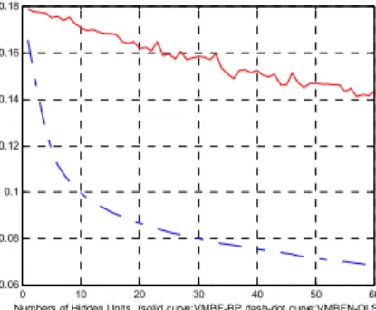
0 10 20 30 40 50 60 0.06 0.08 0.1 0.12 0.14 0.16 0.18
Numbers of Hidden Units (solid curve:VMBF-BP,dash-dot curve:VMBFN-OLS)
Figure 4.2 The root mean square error of the VMBFN training between back propagation and orthogonal least square learning strategy.
From the figures above, the performance of orthogonal least square algorithm is better than the
performance of back propagation algorithm under the same numbers of hidden layer. Because the orthogonal least square method can be employed as a forward regression procedure to select a suitable set of centers from a large set of candidates. At each step of the regression, the increment to the explained variance of the desired output is maximized. So the orthogonal least square approach provides an efficient learning algorithm for fitting adequate RBFN network.
4.2 Testing Result
In the experiments of this section, we use several different numbers of training patterns to train the RBFN and VMBFN with orthogonal least square algorithm. All the experiments use the same numbers of the hidden layer. According the table below, we can find the result in Table 4.1 shows the performance of VMBFN is better than RBFN, even the numbers of the training set are just 310. So we can say that the Von Mises function has the better characters for fitting a spatial characteristic function.
NUMB ERS OF TRAI NING SET RMS ERRO R OF THE SCF USING VMBF RMS ERROR OF THE SCF USING RBFN RMS ERROR OF THE HRIR USING VMBF RMS ERROR OF THE HRIR USING RBFN 700 0.0588 0.0617 0.0213 0.0222 690 0.0824 0.0882 0.0285 0.0303 610 0.0962 0.1017 0.0329 0.0347 510 0.1013 0.1036 0.0346 0.0353 410 0.1052 0.1058 0.0351 0.0355 310 0.1067 0.1069 0.0363 0.0364 Table 4.1 The results of testing error for VMBN with OLS and RBFN with OLS.
4.3 The Implementation of HRIR System According to Figure 4.3, the RMSE of VMBFN is smaller than RBFN. So we use the VMBFN with learning strategy of orthogonal least square to train spatial characteristic functions as our 3D surround system. 0 10 20 30 40 50 60 0.06 0.08 0.1 0.12 0.14 0.16 0.18
Numbers of Hidden Units (solid curve:VMBF,dash-dot curve:RBFN)
Figure 4.3 The root mean square error of training SCFs between VMBFN and RBFN.
We use 60 numbers of hidden units to record our parameters. The original Kemar HRIR database quantity of data is
710 locations × 128 points impulse response = 90880 Then the quantity of our parameters is
60 hidden units × (14 parameters of hidden layer to output layer+3 parameters of inputs layer to hidden
layer)+14×128 eigentransfer functions = 2812 So the compress ratio is
(
)
96.9%90880 2812
90880− =
The simulated HRIR is linear combined with the first fourteen eigentransfer functions and the output from our VMBFN. Then we synthesize the sound. The original sound must be convolved with the appropriate pair of the simulated HRIRs and then presented to the listener binaurally. Usually this is done using headphones. The apparent source position can be changed by selecting the appropriate pair of the simulated HRIRs. However, to prevent clicks in the output, it is necessary to perform some sort of interpolation to smooth the transition. So we must use smaller interval of azimuth and elevation than the interval of Kemar HRIR database as the input of our VMBFN. Then we can synthesize 3D surround sound by out system.
5. Conclusion
A simplified model for HRIR is developed and has been implemented in a network to simulate the sounds. The model avoids minimum phase approximation by directly representing the impulse response of HRTF. Furthermore, the only operations involved in reconstruction of the HRIR are real multiplication and real addition, which means the cost of computation is low. The spatial feature extraction and VMBF network are used to reduce the storage size of HRIRs. Through simple combinations of these extracted parameters, we can get the simulated HRIR. So we believe that our method is an efficient way to virtual acoustic space implementation for human.
二、三維立體影像重建之研究
Abstract
In this project, a neural-network-based adaptive hybrid-reflectance model is proposed for 3-D surface reconstruction. The neural network combines the diffuse component and specular component into the hybrid model automatically. We can consider the characteristic of each point individually and solve the problem of variant albedo. The pixels of the 2-D image are fed into the multi-layer neural network and we can obtain the normal vectors of the surface through supervised learning. Then enforcing integrability method is used for the reconstruction of 3-D objects from the obtained normal vectors. In order to test the performance of our proposed algorithm on the facial images and other images of general objects, we design and construct a photographing environment to satisfy the requirement of the proposed method. To make the strength of different light sources illuminating to the photographed objects equal, the photographing environment is constructed as a hemisphere structure. In order to synchronize the capturing action with the trigger of the electronic flashes, we also design a control board to control the electronic flashes. With this photographing environment, we can modify the direction of illuminant source easily and capture images under variable illumination in a short time. Finally, four
experiments are performed to demonstrate the performance of the proposed method. The advantages of our method are summarized as follows: (1) By the learning ability of neural network, we don’t need to know the illuminant direction in advance. (2) The individual characteristic of each point on the surface is considered. (3) The problem of variant albedo is considered to avoid the distortion of surface reconstruction. (4) According to the experimental results, our neural-network-based adaptive hybrid-reflectance model can be applied to more general objects and achieve better performance for surface reconstruction.
1. Introduction
Shape recovery is a classic problem in computer vision. The goal is to derive a 3-D scene description from one or more 2-D images. The techniques to recover the shape of an object are called shape-from-X techniques, where X is the specific information and can be shading, stereo, motion, texture, etc. Shape recovery from shading (SFS) is a major approach of the computer vision that deals with 3-D shape reconstruction of an object from its gradual variation of shading in 2-D images. When a point light source illuminates an object, since the normals corresponding to different parts of the object’s surface are different, they will appear with different brightness. We make use of the spatial variation of brightness, referred to
shading, to estimate the orientation of surface and then
calculate the depth map of the object. The recovered shape can be expressed in terms of the depth , the surface normal vector , the surface gradient , or the surface slant and tilt.
The SFS approach is firstly proposed by Horn in the early 1970s and is further improved by himself and Brooks. It has received considerable attention and several efforts have been made to improve the performance of recovery.
To solve the SFS problem, it is important to study how the images are formed. A simple model of image formation is the Lambertian model in which the gray intensity of a pixel in the image depends on the light source direction and the surface normal. The classical methods to solve the SFS problem are employing the conventional Lambertian model and minimizing the cost function that consists of the brightness constraint, the smoothness constraint, the integrability constraint, the intensity gradient constraint, or the unit normal constraint. Since solving the nonlinear optimization problem requires a long computational time and it often suffers difficulty in converging to the optimum solution, the approaches of direct shape reconstruction were proposed. All these approaches require an additional smoothness constraint in the cost function.
Ruo Zhang divided the SFS techniques into four groups: minimization approaches, propagation approaches, local approaches, and linear approaches. Minimization approaches obtain the solution by minimizing an energy function. Propagation approaches propagate the shape information from a set of surface points to the whole image. Local
approaches derive the shape based on the assumption of surface type. Linear approaches compute the solution based on the linearization of the reflectance map. Ruo Zhang compared these four kinds of SFS techniques with respect to CPU time and accuracy to realize the advantages and disadvantages of these approaches. It was found that none of the algorithms has consistent performance for all images. They work well for some images, but perform poorly for others. It was concluded that, in general, minimization approaches are more robust, but the other approaches are faster. In order to achieve high performance of 3-D reconstruction, the minimization approach is used in the training stage of our method.
2. Fundamental Reflectance Model There are mainly two kinds of light reflection considered in computer vision: diffuse reflection and specular reflection. Diffuse reflection is a uniform reflection of light with no directional dependence for the viewer. On the contrary, the specular reflection obeys Shell’s law, i.e., the light reaching the surface is reflected in the direction having the same angle.
2.1 Pure Diffuse Reflectance Model
Lambertian surface is the surface having only diffuse reflection, i.e., the surface reflects light with equal strength in all directions, and appear the same brightness in any viewing directions. The brightness of a Lambertian surface is proportional to the energy of the incident light. The amount of light energy falling on a surface element is proportional to the area of the surface element as seen from the light source position (the foreshortened area). The foreshortened
area is a cosine function of the angle θ between the
surface orientation (normal vector) n and the light
source s. The diffuse reflectance model is called
Lambertian model in general and it is used to
represent a surface illuminated by a single point light source as
( ) ( )
(
x,y , x,y)
max{L( ) ( ) ( )
x,y x,y x,y, }Rd n α = α n s 0 .
(2-1)
2.2 Pure Specular Reflectance Model Specularity only occurs when the incident angle of the light source is equal to the reflected angle and this component is formed by two terms: the specular spike and the specular lobe. The specular spike is zero in all directions except for a very narrow range around the directions of specular reflection. The specular lobe spreads around the direction of specular reflection.
The simplest model for specular reflection is described by the delta function:
) ( B Rs= δ θs−2θv , (2-2) where s
R is the speuclar brightness, B is the strength
of the specular component, s
θ is the angle between the light source direction and viewing direction, and
v
θ is the angle between the surface normal and viewing direction.
2.3 Hybrid Reflectance Model
As far as practical application is concerned, it is not enough to considering only the diffuse component
or the specular component single-handedly. In general, most surfaces are neither pure Lambertian nor pure specular, and their reflection characteristic is the mixing of these two reflection components. As a result, hybrid reflectance model was presented. It used a linear combination of the diffuse intensity and the specular intensity by a constant ratio:
R
( )
x,y R( )
x,y ( )R( )
x,y s d hybrid =µ + 1−µ , (2-3) where( )
⋅ hybridR is the total intensity of the hybrid
reflectance model, Rd
( )
⋅ and Rs( )
⋅ are the diffuseintensity and the specular intensity, µ is the
combination ratio for the hybrid reflectance model. 3. The Neural-Network-Based Adaptive Hybrid-Reflectance Model for 3-D Surface
Reconstruction
Although the existing hybrid approaches have already considered the diffuse and the specular reflection, they combine these components by constant ratio for all points on the surface. There are some problems for the conventional approaches. First, they can’t determine the proper ratio between the diffuse and the specular components. In the conventional method, the ratio is obtained by trying in several illuminant conditions and finding an optimal value in the experiments. If the object is changed, then they must try again by the same steps. This may wastes a lot of time and the results may not be correct. If they don’t change the hybrid ratio and use it for all objects, this is unreasonable and it will produce distortion as reconstruction. Second, the characteristic of each position on the surface may not be the same and we should deal with them individually. For example, the brow of human face is usually smooth and flat, and the nose is usually sharp. Thus we should consider different hybrid ratio in these regions. But the conventional hybrid methods use the same hybrid ratio for the whole surfaces, it will lead to ill-reconstruction for complicate surfaces.
Undoubtedly, it is hard to determine the proper hybrid ratio of diffuse and specular components for different surfaces in advance. Therefore, in this project, we propose a novel neural-network-based hybrid-reflectance model and the hybrid ratio of diffuse and specular component is regarded as adaptive weights of neural network. The supervised learning algorithm is adopted and the hybrid ratio for each point is updated in the learning iterations. After the learning process, we will obtain the proper hybrid ratio. In this manner, we will not trouble about the combination and we can integrate diffuse component and specular component intelligently and efficiently.
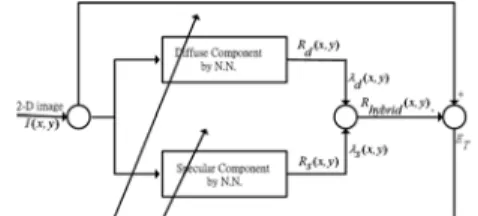
hybrid- reflectance model.
The schematic block diagram of our proposed adaptive hybrid-reflectance model is shown in Fig. 1. The structure diagram consists of the diffuse part and the specular part. They are used to describe the characteristic of the diffuse component and specular component of our adaptive hybrid-reflectance model, respectively, by two neural networks with similar structure of neural network. The composite intensity
hybrid
R is obtained by using the adaptive weights
) y , x ( d
λ and λs(x,y) to combine the diffuse
intensityR and the specular intensityd R . The inputs s
of the system are 2-D image intensity of each point and the outputs of system are the learned reflectance map.
3.1 The Variant Albedo Effect
The conventional SFS methods assume that the object’s surface has constant albedo. When solving the SFS problem, they ignore the effect of the albedo. Consequently, they can’t be applied directly to the images that their object’s surface has variant albedo.
In this project, we calculate the rough-albedo value first for each pixel and adjust the intensity value for each pixel by dividing by the corresponding rough-albedo value. Since the intensity value at each point is just the composite albedo value multiplied by the rest term in the irradiance equation, the effect of albedo variation will be canceled by the intensity adjustment. Then the shape distortion of objects with variant albedo can be solved and obtain the correct depth map.
Fig. 2 shows the reconstructed results of a synthetic sphere with two albedo values on the different regions. The reconstructed result of the conventional method obtains wrong depth estimation as shown in Fig. 2(b). The reconstructed result of the proposed method more approximates to the original shape of the sphere as shown in Fig. 2(c).
Fig. 2 (a) The image with different albedo on the same surface. (b)The reconstructed result by the conventional method. (c)The reconstructed result by the proposed method.
3.2 Diffuse Component of the Hybrid Reflectance Model
The structure of the symmetric neural network used to simulate the diffuse reflection model (as shown in Fig. 3) is proposed. The input and output of the symmetric neural network is like a mirror in the center layer and the number of input nodes is equal to the number of output nodes, therefore, we call it as the symmetric neural network. We separate the light source direction and the normal vector from the input
2-D images in the left part of the symmetric neural network and then we combine them inversely to generate the reflectance map for diffuse reflection in the right part of the network.
Fig. 3 The structure of the symmetry neural network for diffuse reflection model
3.3 Specular Component of the Hybrid Reflectance Model
The energy of specular component is maximum when incident angle of the illumination direction is equal to viewer’s angle and it decreases rapidly when the angle far away the incident angle of the illumination. By physical observation, Phong proposed the reflected intensity function for specular
reflection as (cosφ . When r is larger, the plot of )r
r
)
(cosφ is more closing to the y-axis and the cross
area by the contour of (cosφ is smaller. Therefore, )r
the parameter r is related to the degree of specuarity and it can be use to represent the roughness of the surface. If the surface is rougher, its reflection is approximate to diffuse reflection and its parameter r
should be smaller. Otherwise,
r
should be larger forsmooth surface.
Based on the concept, specular reflection R is s
calculated from normal vector n and half-way vector
h by
( ) ( )
(
)
(
( )
) (
r)
r s x,y , x,y x,y , (x,y) cos R n h = <n h > = φ , (3-1)where
φ
is the angle between normal vector n andhalfway-vector h. If the viewer observes the surface just at the reflected direction, then h equals to n, that
is
φ
=0. In this situation, the observed energy isstrongest and this corresponds to the phenomenon of specular reflection.
3.4 The Adaptive Hybrid-Reflectance Model The complete structure of the adaptive hybrid- reflectance model is shown in Fig. 4. The total intensity of the adaptive hybrid-reflectance model is expressed as the following equation:
,
k k k k d s s d k hybridR
R
R
=
λ
+
λ
(3-2) where k d λ and λskis the adaptive combination ratio between the diffuse and specular intensities in our hybrid model. In order to get the proper ratio of each points,
k
d
λ and λskare regarded as the weights of the
neural network and they can be determined after the training of the network.
Fig. 4 The complete structure of our neural network.
3.5 The Training of the Proposed Model The back-propagation method is used for the supervised learning of our method and our goal is to minimize the error function
(
)
2 1∑
=−
=
m i hybrid i TR
D
E
i , (3-3)where m is the number of total pixels of the 2-D image.
i
hybrid
R is the ith output of the neural network. D is i
the ith desired output and it is equal to the ith intensity of the original 2-D image. For each 2-D image, starting at the input nodes, a forward pass is used to compute the activity levels of all the nodes in the network to obtain the output. Then starting at the output nodes, a backward pass is used to compute
ω ∂
∂ET for the hidden nodes. Assuming that
ω
is theadjustable parameter in the network, the general update rule used is
ω
ω
∂
∂
−
∝
∆
E
T , (3-4)(
)
( )
∂ ∂ − + = +ω
η
ω
ω
t 1 t ET , (3-5)where
η
is the learning rate.3.6 3-D Surface Reconstruction from the Normal Vectors
In general, the surface z(x, y) can be represented as:
(3-6)
where ω=
( )
u ,v is a two-dimensional index wherethe sum is performed, Ω is a finite set of indexes,
and
{
φ(
x ,y ,ω)
}
is a finite set of basis functions which are not necessarily mutually orthogonal. Thepartial derivatives of z , can also be expressed
( )
x yin the same way, that is
(3-7)
(3-8)
where and .
Suppose we now have the possibly nonintegrable )
, (
ˆ x y
zx and zˆy(x,y). We can express these partial
derivatives as
(3-9)
(3-10)
In order to enforce integrability, we would like to find )
, ( yx
zx and zy( yx, )which are a set of integrable
partial derivatives to approximate zˆx(x,y) and
) , (
ˆ x y
zy , respectively. In other words, we want to
solve the equation
(3-11)
If a possibly nonintegrable estimation of surface slopes zˆx
( )
x,y and zˆy( )
x,y is given, a method has been proposed for finding the expansion coefficients c( )
ω as: , for( )
∈Ω = u,v ω , (3-12) whereFinally, the surface depth can be calculated by
performing inverse 2D-FFT on the coefficients c
( )
ω .A schematic block diagram of our method for 3-D surface reconstruction is shown in Fig. 5. The top five blocks of Fig. 5 are corresponding to the learning process of the proposed hybrid-reflectance model and the rest blocks represent 3-D surface reconstruction from the obtained normal vectors. The proposed algorithm corresponding to Fig. 5 for the SFS problem is also summary step by step in Fig. 6.
4. Experimental Results and Analysis Some experimental results are shown in this seciton. First, images of the synthetic objects are used for testing. The estimated depth map is compared with the true depth map to examine the performance of reconstruction.
In the second experiment, images corresponding to real surfaces of human faces are used for testing. Those images are downloaded from the Yale Face Database B. Fig. 7 shows the reconstructed results of the proposed method. Fig. 8 and Fig. 9 show the reconstructed results of human faces and general objects captured by the photographing environment.
( )
x,y c( ) (
x,y,)
, z∑
ωφ ω Ω ∈ = ω( )
x,y c( ) (
x,y,)
, zx ω x ω ωφ
∑
Ω ∈ =( )
x,y c( ) (
x,y,)
, zy ω y ω ωφ
∑
Ω ∈ =(
x y)
( )
x x =∂φ ⋅ ∂ φ , ,ω φy(
x,y,ω)
=∂φ( )
⋅ ∂y( )
x
,
y
cˆ
( ) (
x
,
y
,
)
,
zˆ
xω
xω
ω 1φ
∑
Ω ∈=
( )
x
,
y
cˆ
( ) (
x
,
y
,
)
.
zˆ
yω
yω
ω 2φ
∑
Ω ∈=
. )) y , x ( zˆ ) y , x ( z ( )) y , x ( zˆ ) y , x ( z ( y , x x x y y c min∑
− 2+ − 2( )
(
x
,
y
;
)
dxdy
,
p
x=
∫∫
x 2ω
ω
φ
py( )
=∫∫
y(
x,y;)
dxdy. 2 ω ω φ( )
( ) ( )
( )
( ) ( )
( )
ω ω ω ω ω y x y x p p c p c p c + + = ˆ1 ˆ2 ω ωFig. 5 Block diagram of the proposed reconstructed method.
Fig 6. Summary of the proposed algorithm for SFS problem.
TABLE 1 The absolute mean errors between estimated depth and desired depth of sphere surface. Mean absolut e depth error The diffuse reflectan ce model ([1]) The specular reflectan ce model ([2]) The hybrid reflectan ce model ([3]) Propose d reflectan ce model Consta nt albedo 0.0245 0.0253 0.0240 0.0248 Varian t albedo 0.0286 1.8514 1.7328 0.0283 TABLE 2 The absolute mean errors between the
estimated depth and the desired depth of sombrero and vase.
Mean absolut e depth error The diffuse reflectan ce model ([1]) The specular reflectan ce model ([2]) The hybrid reflectan ce model ([3]) Propose d reflectan ce model Sombre ro 0.0374 1.6823 1.6508 0.0366 Vase 1.2162 0.8937 0.8337 0.0963
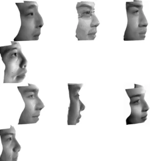
Fig. 7 The reconstructed results of Yale Face Database B by the proposed method.
Fig. 8 The reconstructed results of our laboratory members by the proposed method.
Fig. 9 The images of the first row are the original 2-D images and the images of the second row are the reconstructed results of general objects by the proposed method.
5. Conclusions and Discussions
In this project, a novel 3-D reconstruction method is proposed. This method considers the diffuse reflection component and the speuclar reflection component of the reflectance model simultaneously. We use two neural networks with similar structure to simulate them separately and combine them with the adaptive ratio for each point. The proposed model can be used to generalize the characteristic of the real objects, and the obtained normal vectors of the surface are also applied to 3-D surface reconstruction by enforcing integrability approach.
We also consider the influence of variable albedo and try to reduce the distortion due to variable albedo effects. To cancel the effect of albedo variation, we adjust the intensity value for each pixel by dividing the pixel’s intensity by the corresponding rough-albedo value. Then these intensities are fed into our neural network to learn the normal vectors of the surface by the back-propagation learning algorithm. The critical parameters, such as the light source and the viewing direction and so on, are also obtained from the learning process of the neural network.
In addition, the influence of illuminant positions and angles on the reconstruction performance of our method and how to find the better combination of shaded images for fine reconstruction are also discussed. It is concluded that we should use three images at least for fine reconstruction. However, the reconstructed results that use more than three images are not necessarily better than the reconstructed result that uses three images. Based on the conclusion, we use three 2-D images to reconstruct the surface of a 3-D object in the proposed method and we can reduce the unnecessary calculation.
The contributions of the proposed method are summarized as follows:
1. In the past, we have to know the locations of light sources first for solving the SFS problems. But this is not practical in the real situations. In this project, we used the images under three different light source locations to solve this problem. In our method, we can still obtain a very good result even if the locations of light sources are not given.
2. In this project, we consider the changes of the albedo on the object surface. So, we can also get a good reconstruction results of the human faces and general objects with variant albedo.
3. Applying the proposed model combined with supervised training procedure for solving SFS problems does not need any special parameters and the smoothing conditions. It is easier to converge and make the system stable.
4. The proposed method applies the adaptive combination ratio for each points of the surface to compose the diffuse intensity and specular intensity. In this manner, the different reflecting properties of each point are considered to achieve better performance of surface reconstruction.
From the experimental results, our proposed method can reconstruct the object well and it also indicates that our method is better than the conventional approaches indeed. There are still some aspects to be improved in the future, such as the influence of object size, some critical surface, and so
on. In addition, the present researches considered the
linear combination of the diffuse components and the specular components by some way. In the future, we could study a single nonlinear reflection model to consider these two components efficiently and directly.