An automatic Petri-net generator for modeling a flexible manufacturing system

(1)

An Automatic Petri-Net Generator

for

Modeling

a

Flexible Manufacturing System

Tien-Hsiang

Sun

Li-Chen Fu

Department of Computer Science and Information Engineering

National

Taiwan

University, Taipei, Taiwan,

R.O.C.

Abstract

Petri-Net is widely used in the field of modeling a flexible manufacturing system (FMS) because of its intrinsic features such as concurrency, uynchronization, conflict, and event- triggering. But designing a Petri-Net Model for an FMS is extremely tedious and difficult for debugging. Therefore, an automatic Petri-Net generator which can generate a bug-free model for an FMS is rather useful and practical. In this paper, a systematic method t o construct a Timed Place Petri- Net model for modeling an FMS is proposed, and is imple- mented as an Automatic Petri-Net Generator, with a Graphic User Interface, through which a user can input the system information of a practical FNS, such as the number of automated guided vehicles (AGVs), the number of machines, and their geometric relationship, a8 well as process flows of parts

to be processed. Then, this generator will use these pieces of d ata to generate the corresponding Petri-Net Model.

1 Introduction

Petri-Net has evolved into an elegant and powerful graphi- cal modeling tool for asynchronous concurrent event-driven systems. T h e wide ranging application areas of Petri-Net include communication protocols [IS, 191, distributed s y s terns [20], database [22], multi-processor memory systems

[21], complier and operating system [23, 241, formal languages

[25, 261. In additional, Petri-Net are very useful tool for mod-

eling [4, 5 , 171, simulation [6, 171, and scheduling [?] of dis-

crete event systems, such as flexible manufacturing systems, and also for designing and implementing controllers for man- ufacturing [11, 121. In the earlier work of our laboratory, a Petri-Net model is built to model the detailed behavior of an

FhfS and a schedule is generated by running an A* search on the Petri-Net model. T he result is quite satisfactory.

However, designing a Petri-Net model for an FMS is ex- tremcly tedious and difficult for debugging. For this reason, it is extremely necessary to have a Petri-Net generator to generate a bug-free Petri-Net model for an FMS. A genera-

to1 is a program that can generate some specified program

or da t a structure from the relevant system information input

by uscrs. For example, in a UNIX system, there are Yacc as

Pasei Generator and Lex as Scanner Generator. And there is

also some similar software in the context of Petri-Net, for example, Design/CPN is an interactive computer tool for per- forming modeling and simulation with Color Petri-Net In this paper, a systematic method to construct a Timed Place

Petri-Net (T PPN) model for modeling an FMS is proposed, which inherits some excellent features in modeling from our early work but is now more thoroughly and systematically refined. This systematic modeling method is implemented as an automatic Petri-Net generator (APNG). The term “Auto- matic” means that users d o not need to design the Petri-Net model by themselves, but the Generator will create

dl

kinds of Petri-Net model of any

FMS

subject t o users definition. By using such a generator, building a Petri-Net model of a FMS is no longer a difficult and time-consuming task. User only need to input the system information of a practical FMS, such as the number of automated guided vehicles (AGVs), the number of machines, and their geometric relationship, as well

as process flows of paxts to be processed. We also develop a graphic user interface to help user input these information more easily.

The organization of this paper is described as follows. In Section 2, the detailed systematic Petri-Net modeling method will be introduced. In Section 3, a practival example of using the proposed machinery will be presented. FinalIy, conclu- sions are provided in Section 4.

2 Systematic Modeling Method

In this paper, we select the Timed place Petri-net (TPPN), in which time is associated only with places and all transitions are instantaneous, to model our manufacturing systems. Because the markings of the TPPN are deterministic during the evolution of the firing sequence from initial marking, we can undoubtedly use the markings of the T P P N to describe the states of the system and all the reachable markings can represent the state space of the modeled system

Fig. 1 shows the hierarchical view of the entire system model, which contains two major sub-models. One is called

TI ansportation Model and the other is called Process-Flow Model. Th e objective of the Transportation Model is to model the behavior of the AGV traveling from the current stop to its destination stop, and that of the Process-Flow Model is to describe the behavior of the part routing and rehource assignment. The two sub-models, of course, are interactive with each other to undertake the necessary actions in response to the triggering from another.

The Transportation Model is decomposed into several sub-

modules, each with different characteristics. One is Trans- pcrrtat,ion Layout Module, which models the relative positions

oI AGV stop points and the path segments connecting adjacent stop points, and the other is Movement Control Module,

(2)

which models the routing control rule of an AGV moving from one stop point to another. However, if there is more than one

AGV in the system, the Push Control Module has to be additionally included in order to avoid the AGV collision problem. Each of the above modules is further composed of several micro modules called Transportation Unit Module, Movement Control Unit Module, and Push Control Unit Module. Sim- ilarly, the Process Flow Model is compesed of various unit modules : (1)

AGV

Link Unit Module is used when a part need t o b e transported by AGVs. (2) Cell Link Unit Module is t o describe t h e cell material handling system (robot, rail guided vehicle) when the system consists of several machine cells. (3) Virtual Link Unit Module characterizes the situation where two adjacent operations can be processed by th e same machine, (4) Job Start & End Module describes the pool of readily processed parts and of finished parts of a job.

( 5 ) Buffer Link Unit Module is used to represent the situa-

tion where a part is moved from a machine input buffer into the machine for processing and a processed part is moved out from the machine to its machine output buffer.

Th e entire model is synthesized by these sub-modules or modules and micro modules which are in conjunction with one another using common places, and hence every place in the model will be associated with a unique name.

2.1 Modeling

of

a Transportation

Sys-

tem

T he Transportation Model can be decomposed into several micro-models (called modules), each with different characteristics, one is Transportation Layout Module and the other is Movement Control Module. However, the Push Control Module has t o be additionally included if the number of t h r material handling carriers is greater than one, i.e., if a multiple-AGV system is installed. The following are detailed descriptions of each of these micro-models and we will provide algorithms t o show how the Petri-Net generator can automatically generate each of these micro-models.

Transportation Layout Module

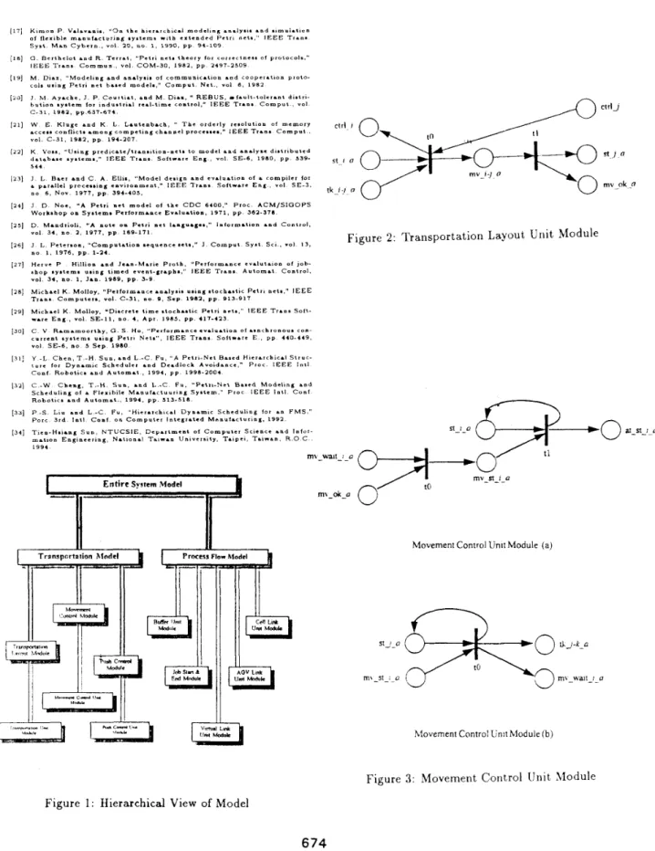
T h e purpose of the Transport Layout Module is to model the layout of the transportation system. The basic concept of this model is described as follows. When an AGV needs t o move from the current stop t o the next adjacent stop, it needs

to receive a ‘ticket’ of movement first to know its destination and then acquires the control right of the next adjacent stop to make sure that stop is free a t the moment. If both of these conditions are satisfied, it can thus start its traveling to the next adjacent stop. At the same time, the control right of the current stop will be released to allow another AGV to use it

as a destination or pass-by stop.

Algorithm 1 shows how the generator can automatically generate the full Transportation Layout Module. Some con- stants used in the algorithms of this paper are described as

follow :

0 N - S P is the total number of stop points of the trans-

portation layout of an FMS.

0 N A G V is the total number of AGV of an FMS.

0 S-ARC is the

of an FMS. set of arcs of the Layout Directed Graph

Algorithm 1

: Construct-Transportationlrayout-Module Step 1:

FOR

(I = 1 T O N A G V Step 2: Step 3: Step 4: NEXT Step 5: NEXT

FOR

every (i, j ) E S A R C

Construct a Transportation Layout Unit Module

(as shown in Fig. 2)

Th e notation of places used in Fig. 2 are explained as fol-

1) st-La, represents the stop at a workstation. A to-

ken in s t i a means AGV a is now staying at stop lows:

1.

2) ctrl-i, represents the control right of stop a . 3) tk -i - ja , represents a ticket t ha t drives AGV a to

4) m v-i - j a, represents the moving of AGV a from

5) mv-oka represents the status of completing the move from stop i to stop 1.

stop i to j.

AGV movement along a segment path.

It is noteworthy that up t o now the Transportation Model has already embedded a control rule into it so that no vehicle collision problem will ever occur.

Movement Control Module

Th e Movement Control Module corresponds to the decision- making Petri-Net model for AGV routing. Each time when AGV a wants t o move from the current stop to some other stop, it must determine its route of movement first. The determined route can be sent t o the Transportation Layout Module through ‘ticket’ places tk-a-ja to entail the AGV a to move along that route. Therefore, for each stop, we need to have a corresponding Petri-Net model to take care of the routing decision, guiding the traveling path from other stops to it.

Because there may be more than one path from stop point

J to stop point i, the Petri-Net generator must find all paths

from each stop point to a specified stop point. This can be done by traversing the Layout Directed Graph, and algorithm

2.1 shows how this is done by the generator and Algorithm

2.2 describes the procedure of generating Movement Control Module.

Algorithm

2.1

:

FindAllPath-To-StopPoint(i)

Step 1: ARRAY S t a t u s [ l , .

. .

, N S P ]

Step 2: MATRIX A n s w e r [ l , .

. . ,

N S P ] [ I , . .

.

,

N - S P ]

Step 3: Initialize STACK

Step 4: Initialize Status[1, .

. . ,

N S P ]

=

0

Step 5: Initialize Answer[l,.

. .

, N S P ] [ a , . .

.

,N-SP]

=

0

Step 6: PUSH i into STACK Step 7: Status[i]

=

1

Step 8: WHILE STACK is not empty Step 9:

Step 10: Statuslj] = 2

P O P j out of STACK

(3)

Step 11: Step 12: Step 14: Step 15: A n s w c r [ k ] b ] = 1 Step 16: END

IF

Step 17: NEXT Step 18: END WHILE Step 19: RETURN Answer

FOR

k

= 1 T O N - S P

IF (t,j) E S A R C AND Status[t]

=

0 THEN

Step 13: Stalus[k] = 1

PUSH

k

into STACK

The meaning of the array Stafus and the matrix Answer

0 Siatus[i]

=

are respectively described as follows :

0 : point i has not been traversed;

1 : point i has been traversed but not expanded yet;

2 : point i has been traversed and expanded.

0 Anawer[i][i] =

0 : there is no arc from point i to point j or the arc is no use for the traversal;

1 : the arc from point i to point j is useful in the traversal

The notations of places which are different from those in the Transportation Layout Unit Module are described as follows.

1) Th e place m v s t - i a represents the request of AGV

a moving from the current stop to stop i.

2) The place atst-i-o represents the request of AGV movement from the current stop t o stop i is fulfilled.

3) The place mv-wait-ia means a waiting for the mv-ok-a condition to generate a ‘ticket’ for the next segment path.

Note that m v s t - i n and a t s t i - a places are both control places that are used t o iniorm the Transportation Model to move an AGV to stop i arising from the request made by Pro- cess Fluw Model and then to resume the processing of parts in F’rocess-Flow Model, respectively. The palce mv-wait-i-a is an intermediate place and is used only to wait for the place mv-ok-a to be marked in the Transportation Layout Module after interior firing.

Algorithm 2.2

:

Const ructmovement XontrolModule

Step 1 : MATRIX Path[l,

. .

,

N S P ] [ l , . .

,

N S P ]

Step 2: FOR a

=

1 T O N A G V Step 3 : Step 4: Step 5: P a t h = FindAll-Path-ToStop-Point(:) Step 6: Step 7: FOR i

=

1 T O N S P

Construct a Movement Control Unit Module (a) (Fig. 3 (a))

FOR every 3, k

E

( 1 , .

. .

,

N - S P }

I F P a t h l j ] [ k ] = 1 THEN Construct a

Movement Control Unit Module (b) (Fig. 3 ( b ) ) Step 8: NEXT

Step 9: NEXT Step 10: NEXT

P u s h Control Module

In a production system, the transporting system may have more than one carriers which transport materials among different workstations. Though, there no longer exist collision problems, the traffic j a m problems due to multiple carriers must be considered and solved. The objective of the Push Control Module

is

again t o introduce a control method into the Petri-Net model with an aim to guaranteeing the jam-free condition among carriers.

The method we provide is a way called purh-AGVstrategy, whose basic idea io described aa iollows. When a busy AGV found that a stop on its traveling route was occupied by another freed (idle) AGV, it will send a push command to that idle AGV to ask it to leave that stop. After a ’ticket’

is

sent to that idle AGV, it starts to move to its next adjacent stop and releases the occupancy of its previously residing stop. When that stop

is

completely released, the busy AGV can resume its traveling on the same route path.

The Push Control Module can be constructed based on Push Control Unit Modules, as shown in Fig. 4. Consider every three adjacent stop points. If AGV a

is

a t stop i and AGV b is at stop 3 and AGV a wants t o move to stop j while AGV b is idle, then AGV b will be pushed by AGV a to the other stop point, e.g. stop k. So, this module sends a token to the place tk-j-k-b in the Transportation Layout Module and, when AGV b completes its movement, the module will send a token to m v a k J so as to inform AGV a to start its movement. Algorithm 3 summarizes the procedure of generating the Push Control Module.

Algorithm

3 :

Construct Push-ControlNodule

Step 1: FOR every (i,3)

E

S - A R C

Step 2: Step 3: Step 4: Step 5 : FOR every k

E

(1,.

. .

,

N S P )

IF

( I , k )

E

S - A R C THEN FOR every a, b

E

{ l , .

.

,

N A G V ) , 18

#

b

Construct two Push Control Unit Modules (Fig. 4) : one for AGV a pushing AGV b and the other for AGV b pushing AGV a

Step 6: NEXT Step 7: END

IF

Step 8: NEXT Step 9: NEXT

2.2 Modeling

of

a

Process

Flow

A process flow in manufacturing can be seen as a sequence of part transportations by the material handling system and the transporting system among different workstations, and part processing on numerically controlled NC machines. The

Petri-Net model we proposed to represent the process flow of each part type is called Process-Flow Model, which models the technological precedence constraints for processing parts and normally provides more than one alternative route to accomplish the processing.

There are five micro modules that we use to generate the Process Flow Model, while we now introduce one by one in the following.

(4)

AGV Link Unit Module : is used for describing the situation where a part is transported via the AGV system,

which starts from a call of an AGV to the source stop point, then the loading operation] and commanding the AGV to the goal stop point, and finally ends with the unloading operation. The behaviors of AGV Link Unit Module is that, when a part needs a service of an AGV at stop point t and if there is a freed AGV as well as the target resource (resource-2) is free, then the mod- ule issues a moving command to the Movement Control Module of the Transportation Model by placing a token in the place ''mvst-id' to drive AGV a t o move to the source stop point at which the part is residing. When the movement is complete, the Movement Control Module will then place a token in the place 'at-st-in" and then starts the loading operation, which takes some time. Once the loading operation is done, this module will send another moving command to the Move- ment Control Module by placing a token in the place " m v s t - j a to drive AGV a to move to stop point j and at the same time release the resource-1. Similar to the above description, when the movement is done, there is a token in the place " a t s t - j a " , which is then followed by the unloading operation. Finally, when the unloading operation is completed, the mission for the AGV in the AGV Link Unit Module is considered accomplished.

Cell Link Unit Module : is used for describing the situation where a part is transported by the Cell Material Handling System, e.g. (Robot or RGV), when a part in the Cell needs to be transported from a location to another location in the cell.

Vh-tual Link Unit Module : is used €or describing a situation where a part can be processed with two successive operations in the same machine.

J o b S t a r t & End Module : is used to symbolize the start- ing and the ending of a Job.

Buffer Unit Module : is used for describing the situation

where a part is passed from the machine input buffer into the machine for operation, and is then passed to the machine output buffer when the operation is done.

By using these five unit modules, a process flow of a job can be easily mapped to the corresponding Petri-Net. The algorithm to build the Process Flow hlodel, because of the limiting space, is not presented here and can be found in [34]

3 Implementation

The implementation of the systematic Petri-Net modeling method is through a program called Automatic Petri-Net Generator. By further, we also combine the generator with a search based scheduling method which is proposed by our earlier work [32]. The integrated version of the above mod- eling as well as scheduling programs is design by an Object- Oriented method and programming with

C++.

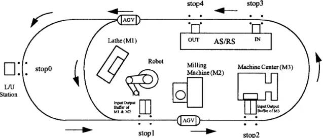
Compilation is done via G N U C++ Vex 2.5.7 on Sun SPARC I1 Worksta- tion.

of Department of

Me( hanical Engineering at National Taiwan University as our target system. The components of this

FMS

contains an L / U

station, a robot, an AS/RS, a Lathe machine, a Milling ma- chute, a Machine Center and two AGL's The layout of this

We use an FhiS in Autoniatioir Lab.

target system is shown in Fig. 5. Note that, the Machine chine are in the robot cell and has no input and output buffer, each of them using the common input and output buffer of the robot cell. T h a t is, parts which enter or leave Lathe or Milling machine must be transfered by robot. Table 1 r e p resents the job requirements of an example. By the running the Automatic Petri-Net Generator, the final Petri-Net model contains of 377 places, 429 transitions, 838 transition output arcs, 802 transition input arcs. After the model is generated, the search algorithm next searches on the reachability graph, and finally the program outputs a schedule.

Center has input and output buffer, Lathe and Milling ma-

4 Conclusion

In this paper, we proposed a systematic Petri-Net modeling for an FMS. Th e entire model is composed of two sub-model, one is Transportation Model and the other is Process Flow model. The objective of Transportation Model is to model the behavior of AGV traveling from the stop a t which i t cur- rently stays to its destination stop, which must also ensure that the collisions are avoided. And, the Process-Flow Model is used to model the behavior of the part routing and resource assignment several algorithms are used to construct both Transportation Model and Process Flow Model, which then comprise the Automatic Petri-Net Generator (APNG). An A' search based scheduling method was also proposed to provide an appropriate schedule.

References

C. A . Petri, "Kommw.ikaIiom mil Automaten," P b D thesis, Umive*.ily 01 Boa., Oermrmy. 1962.

1. L . P e t c r . ~ . , "Pelri nets." C o m p u l . Surrey., vol. 9 , S e p . 1977

T . Murat., "Petri Nets i Properties, Ana1y.i. and Applis.liani." P m c . IEEE. v o l PORC-77. no. 4 , p p . 541-580, Apr. 1989

Y . Narahrri and N. V i . r a n r d h a m , " A Pelri net a p p t o r c h l o modelimg and anr1y.i. of flexible manmfacluring bystem." A n n . Operatio. R e i . . vol. 3, 1985, p p . 449-473.

C h i n - J u n g T , Li-Chen F . and Y r n g - J c m H . , "Modolims and Simulrliom l o r F l e i i b l e Mamufac1uri.S S y s l e m . *sing Petri Net", T h e s e c e n d Inltrnalional Caoferemcr om Aulom.1ion Technology. pp.31-30. v o l . 4 , 1993.

K . Vcnkalemb, 0. M ~ S O I Y , rnd I . Wu, 'Simulrtion r a d robot scheduling o l a

lust-im-time flexible r u l o m a l o d s y s t e m maims l i m e d Petri Net.". T h e second Imlernrlionrl Comf. Automation Techmology. r o l 4 , p p 75-79, July 1993. C . F . 0 . Bispo, J . J . S. Senlieiro. a n d R. D . Hibbcrd. "Adaptive scheduling for higb-volume .hops*. IEEE Trrn.. R o b o t . Automat , pp.696-706. vol.1.

D e c . 1992.

C . Bispo rmd 1 . Semltciro. " A n cxlemded borison .chcduling d g o r i l h m for t h e job-.hop problem." Porc. 1.1 1.1. Conf. CIM. May 1988.

L. E. Hollorry. 8 . H . K r o g h . uSynlhe.i. of feedback control losic lor L cia..

01 Controlled Pelri Nets". IEEE Trans. A u t o m a t . Conlr , ro1.35. pp.514-523, Mry 1990

L. E. Hollorry, F . H o w r i n . "Feedbrck Conlrol lor s e q u e n c i n g specificrlions

in C o n l r d l r d Petri N e t s " . Proc. IEEE Con(. Robotic. amd A u l o m r t i o n . p p . a + a - a s i . i s a .

D. C r o c k e l l . A . Derrocbers. F . DiCemrc, r n d T Ward " l m p l c m c n l r l i e n 01 r Petri mcl conlrollcr for mashime r o r h l a l i o n , " in P r o c IEEE Roboltc. Automat. C o n t . , 1907. p p . 1061-1067.

M. C. Z h o n . F DiCemrre. r i d D . Rudolph, "Control 01 flexible manulrc- luring syntcm using Petri act.." i n Proc. IFAC Congr , r o l 9. 1990, pp 4 3 - 4 c

E . Kaslurir, F . D C e * r r . and Dcsrocher., "Real-time cumlrol d mmltilevel mrmufrcluring aystem# mains colored Petri met.." in P i o c . IEEE Robotic.

A u t o m a l . Con<., 1980. p p . 1114-1119.

K t i . Lee r m d 1. favml. "Hierrrchicrl redaction m e t h o d lor rnrlyoia and decomposition 01 Pclri n e t s . " IEEE Trans. Sy.1 M a n Cyberm , r o l SMC-15.

K. H . Lee. 1. Favrcl, and P B a p t i s l e . "Generali%cd Petri met rcductiom method," IEEE Tr&ns. S y s l . M a n C y b e r n . . vol. 17, 110 1 , 1917. p p . ?97-

303.

a . 1915, pp. a7a-280.

J . C Gcnlinil a o d D Corbcel, "Coloted r d r p l i v e slruclcd Petri n e t : A 1001

for l h e .ulomaled s y n t h e m ot hier.rchic.1 sonlrol 01 flrribls manutrsluring .y.tcm.,' i n Proc IEEE Robotic. A u t o m r l C o a l . 198-. p p . 1166-1173

(5)

K i m n n P. V d a v a m i . . *'an t h e h i e r a r c h i c a l m o d c l i n g a n d y s i . a n d . ~ m u l r t i c n

o i flexible m a n u f a c t u r i n g aystems w i t h e i t e n d c d P e t r i net.." I E E E T r a n s

Sy.1 M a n C y b c r n , v o l 1n, n o I , 1 9 9 0 , p p 94-109 G . B c r t h c l o l a n d R . T c r r a t , ' " P e t r i n e t . t h e c r y l o r c o r r e c l n e s s o i ~ ~ D I o c o I ~ , ' ' I E E E T r a n s C o m m u n , v o l . C O M - 3 0 , 1 9 8 2 , p p 2497.a509 M . D l a r , "Modclrog a n d an.lyii. 01 ~ o m i n u n i ~ a t i o n a n d c o o p e r a t i o n p ~ o t o - c o l i u s i n g P e t r i a c t based model.," C o m p u t N e t . . v o l 6 . 1 9 8 2 I b u t i o a s y s t e m l o r i o d u . t r i d r e a l - t i m e c o n t r o l , " I E E E Tree. C o m p u t , Y O I C - 3 1 , 1981, p p . 6 3 7 - 8 7 4 .

W E K l u g e and K L. Lautenbach, '' T h e orderly r e ~ o l u t i o n o i memory L C C ~ ~ S c o n i l i c t i a m o n g c o m p e l i n s ch.olrel procca.e.," l E E E T r i o . C a m p u t ,

"01. C - 3 1 , 1982, p p 194-207.

K Vasa, " U a i n g p r c d ~ c r t e / t r ~ n ~ ~ l ~ a n - n e t . t o m o d c l a n d a n ~ l y i e dts1rhbut.d database s y . t e m . . " I E E E Trans. S o f t r a r e E n & , v o l SE-6, 1980, p p . 539-

544

J L B s e r a n d C A. Ellis, "Modcl design and e v d u . t i o n 01 L c o m p i l e r lor

a p a r a l l e l p r c c e . m n ~ e n v i r o n m e n t , " I E E E Trans S o i t r r r c Eng , v o l SE-3, n o 6 , N o v . 1 9 7 7 , p p . 394-405,

J D N o e , " A P e t r i mct m o d c l o f t h e C D C 6 4 0 0 , " P r o c . A C M / S I Q O P S

W o r k s h o p om System. Pcrlormance E v d u r l i o n , 1 9 7 1 , p p 362.378 D. M a n d r i o h . "A n o t e o m P e t r i net I.n&u.&'.," l n l o r m & l t o n and C o n t r o l ,

hl A y a c h e , J . P. C o u r t i a t , rmd M . D i r s , " R E B U S , i a u l t - t o l e r a n t d i s t r b -

3 4 , 10 9 . 1 9 7 7 , p p 189-171.

J L . Pctcrsom, " C o m p u t a t i o n s e q u e n c e n ~ 1 1 , " I C o m p u l Sy.1 Scr , "01 1 3 ,

n o I , 1 9 7 6 , p p . 1-24.

H e r v e P H t l l i o m a n d J e a n - M a r i e P r o t h , " P c r i o r m a n c e c v a l u t * a o n of l o b - s h o p system, u i i n g t t m e d event-graph.," I E E E T r a n s . A u t o m a t Control.

v o l . 3 4 , no. 1. I a n . 1969. p p . S-9

M i c h a e l K . Molloy, '*Periormaoce an.1y.1. u.iog . l o c h a n t i c P e t r i n e t * , " I E E E T r a n s C o m p u t e r . , v o l . C-31, n o e , S c p . 1982. p p . 913-917 M l c h i c l K M o l l o y . 'Discrete l i m e s t o c h a s t i c P e t r i n e t . . " I E E E T r a n s Soft- V L ~ C E n s , vol. S E - 1 1 , no. 4 , A p r . 1 9 8 5 , p p . 417-423 c V Ramnmoarlby, G S H o , " P c r i o r m . n c e ~ v d u a t i o o o i a s n c h r o o o u . c o n - c u r r e n t s y i t e m s u u n g Petri N e t , " , I E E E T r a n s S o l t w r r c E , p p 440-449, v o l S E - 6 , n o 5 S c p 1980 Y .L C h c n , T - H S u n , a n d L -C F u , " A P e t r i . N e t Based H i c r a r c h i c . 1 S t r u c - t u r e for D y n a m i c S c h c d u l e r .nd D e a d l o c k A v o i d a n c e , " P r o c . I E E E l n l l C o n f . Robotic. and A u t o m a t , 1 9 9 4 , p p . 1990-2004 C - W C b e n g , T.-H. S u n , a n d L - C F u , " P e l r t - N r l B a a e d Modelin& a n d Schedulraig o f a F i e x i b i l e M . o u l . c t u u r i n g Syntem," P i o c I E E E l n t l C o n i Robotic. and A u t o m r l . . 1 9 9 4 , p p . 5 1 3 - 5 1 6 .

P - S L i u and L - C . F u , " H i e r a r c h i c a l Dynamic Scheduling l o r r n F M S , "

Porc 3 r d l o l l C o n i o n C o m p u t e r I n t e g r a t e d M a n u i . c t u r r n g , 1 9 9 2 .

T l c n - H . i r n s S u n , N T U C S I E , D e p r r t m r n t oi C o m p u t e r S c i e n c e & a d l n i o r m a t i o n Engineering, N ~ t i o n i l T a i w a n University, T u p e k , T a x r a n . R.0 C 1994

Entire System Madcl

Figure 2: Transportation Layout Unit Module

Movement Control Unit Module (a)

Movement Control Unit Module (b)

Figure 3: Movement Control IJnit Module Figure 1: Hierarchical View of Model

(6)

0:

I

A

J

Station

Figure

4: Push

Control

Unit

Module

Machine Center

(M3)

stop 1

stop2

Figure

5:

System Layout

for

Example

I

Job 1

1 r

Job 2

1

~~~ ~

Table 1 :

Job Requirement for Example 1