3D Indoor Virtual Environment Modeling via Vehicle Navigation and Multi-Camera Image Data Fusion

全文

(1)3D INDOOR VIRTUAL ENVIRONMENT MODELING VIA VEHICLE NAVIGATION AND MULTI-CAMERA IMAGE DATA FUSION Hui-Ping Fan and Wen-Hsiang Tsai Department of Computer & Information Science National Chiao Tung University, Hsinchu, Taiwan, R.O.C Email:whtsai@cis.nctu.edu.tw. Abstract. plication researches have developed techniques for mod-. In applications of virtual reality, it is often required to. eling environments using a variety of sensors and a spec-. usually. trum of techniques. Illingworth and Hilton [1] introduced. time-consuming. In this study, an offline automatic ap-. the principles and methodologies to build a 3-D model. proach to 3-D indoor virtual environment modeling by. world using a variety of sensors and a spectrum of tech-. the way of autonomous land vehicle (ALV) navigation is. niques. For 3-D indoor environment modeling, Lebègue. proposed. An ALV is first driven manually along a path. and Aggarwal [2,3,4,5] developed an integrated system. by a driver to collect environment data using three cam-. to generate architectural CAD models using a mobile. eras mounted on the ALV. The system then generates the. robot. The system consists of a segment detector, a. environment model by a data fusion approach using the. tracker, and a CAD modeler optimized for environments. model learning result from the multiple-view data, per-. with prominent 3-D orientations. Takeshi Shakunaga [6]. forms intelligent post-processing works to create a more. proposed a method by which specific corridor models. complete model, and uses the VRML language to con-. can be recovered from a single image made by a. struct a corresponding 3-D virtual reality (VR) model. well-calibrated camera. The recovery is based on a ge-. automatically. Good experimental results prove the fea-. neric corridor model that covers a wide variety of corri-. sibility of the proposed approach.. dors. Also, Egazzar, et al. [7] investigated modeling of. establish. environment. models,. which. is. Fusion,. indoor environments using a low-cost, compact, ac-. Multi-Camera, Indoor Environment Modeling, Computer. tive-range camera, known as BIRIS, mounted onto a pan. Vision, Virtual Reality. and tilt motor unit. Pan and Tsai [8] proposed an inte-. Keyword:. Vehicle. Navigation,. Data. 1. Introduction Autonomous land vehicles (ALV’s) have attracted intensive research effort in recent years because of its versatile applications. With recent development of computer vision and image processing techniques, more applications of ALV’s have become feasible. Many applications of ALV navigation in environments require a dependable model of the world. However, establishment of environment models is really a time-consuming work. Also, recent interests in virtual reality and multimedia have provided a great impetus to the development of automatic techniques for building graphical models and environments by sensing the real world. Learning of models in these ways is essential, particularly in terms of production times and attaining high fidelity. Many ap-. grated approach to automatic model learning and path generation for vision-based ALV guidance in building corridors.. In. Chen. and. Tsai. [9],. an. incre-. mental-learning-by navigation approach to vision-based ALV guidance in indoor environments was proposed. The proposed learning approach is reliable because of the robustness of the use of the proposed MWGHT (Multi-Weighted Generalized Hough Transform) matching scheme. And the learned environment model can be updated after each navigation session. A new approach to vision-based unsupervised learning of unexplored indoor environments for ALV navigation was also proposed by Chen and Tsai [10]. The ALV can conduct automatic learning of navigation environments without human involvement..

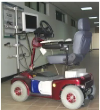
(2) chitecture, as shown in Figure 2.2, including four major. 2. Overview of Proposed System. components, namely, a vision system, a central process-. 2.1. System Configuration An ALV with smart, compact, ridable characteristics, as shown in Figure 2.1 is used as a test bed for this study. It is a commercial motor-driven vehicle modified by adding sensors, electronic controls, an on-board PC, and several power conversion equipments. The ALV can be switched between the manual operation mode or the computer operation mode by the user.. ing unit (the Intel Pentium II 450MHz PC mentioned above), a motor control system, and a DC power system. The vision system consists of the three cameras, a color monitor, and an image frame grabber. The motor control system consists of a main control box with the controller and the motor driver mentioned previously, and two motors. 2.2. Brief Description of Proposed System The goal of this study is to construct an appropriate 3-D model of the indoor environment using the images taken by three cameras mounted on an AVL. The 3-D model data may be used to build a virtual reality environment for many applications (e.g., navigation, visualization, and so on). The proposed approach consists roughly of three stages. The first stage is initial learning, in which the ALV is driven manually along a path decided by a driver. Three images are captured simultane-. Figure 2.1 The ALV used in the experiments.. ously from the three cameras and the control status data In the experiments of this study, we use three cameras. are recorded in each navigation cycle. Then, a certain. to take images with a resolution of 640×480 elements.. off-line procedure is performed to construct the initial. These cameras are mounted at fixed positions on the. model. This is accomplished by calculating the relations. cross-shaped racks of the ALV. More specifically, there. between the ALV and the environment features observed. are two cameras on a crossbar. One camera is attached to. in each learning cycle, and by matching the features with. the left position and the other is attached to the right po-. the partially learned model, followed by the step of fus-. sition, of the crossbar. The third camera is on another. ing the processed data from the three cameras. The sec-. crossbar and is attached to the middle position of that. ond stage is to refine the observed 3-D raw data pro-. crossbar. The lower two cameras are used to grab images. duced by imperfect matching and image processing techniques using data extracted from limited camera views. The third stage is to connect different corridors to. Main Computer. CCD. PentiumⅡ450MHz 128MB RAM 6.4 GB Hard Disk. CCD. complete the model by performing a line-pattern match-. command RS232. Control Box. status. Matrox Frame VGA Display. CCD Video. Grabber. Card. Feedback Signal. ing algorithm and to build the 3-D VR environment. Control Signal. model, using the refined 3-D data. 2.3. Procedure of System Operations. Display Signal. TFT Display. M. M. Rear Wheel. Front Wheel. The system operations are based on a hierarchical approach, which include the following steps: (1) Perform camera calibration for each camera.. Figure 2.2 System structure of the left and the right baselines of the wall in the building corridor, and the upper one is used to grab images of the ceiling of the corridor. The ALV is computer-controlled with a modular ar-. (2) Grab an image from each of the three cameras and save them as an initial model at the initial location. (3) Drive the ALV manually from the initial location and grab three images of the current environment scene. (4) Record the environment images, the counter values of.

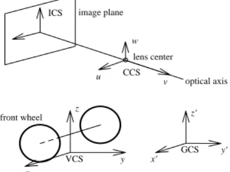
(3) the odometer, and the turn angles of the front wheels. (5) Manually drive the ALV a certain distance and make appropriate turns to keep it in the middle of the corridor. (6) If the ALV reaches the destination, go to (8) to perform off-line processing; else, go to (3) for the next cycle.. model. 3.2. Coordinate System Transformation Four coordinate systems and coordinate transformations are defined here for use in the following sections. They include the camera coordinate system (CCS), the. (7) Perform image processing.. image coordinate system (ICS), the vehicle coordinate. (8) Perform model learning.. system (VCS), and the global coordinate system (GCS).. (9) Generate the overall 2-D environment model.. These coordinate systems are shown in Figure 3.1. Since. (10) Construct a corresponding 3-D VR model.. the origins of the ICS, CCS, and VCS are attached to some points on the ALV, the ICS, CCS, and VCS are. 3. Detection of Environment Features for Model Learning. moving with the vehicle during navigation. On the contrary, the GCS is fixed all the time, and is defined to be coincident with the VCS when the ALV is at the starting. 3.1. Introduction Selecting stable environment features and developing. position in the initial model learning stage.. effective methods to extract these features are the most. The location of the vehicle can be assured once the. important keys to successful model learning. In this study,. relation between the VCS and the GCS is found. Since. the selected environment features come from the base-. the vehicle is on the ground all the time, the z-axis and. lines and ceiling information in building environments.. the z'-axis can be ignored.. Some advantages of selecting features from these sources are listed in the following:. The transformation between the two 2D coordinate systems x-y and x'-y' can be written as follows:. Baselines: baselines are abundant and easily visible in buildings;. (x '. y ' 1) = ( x.  cosω y 1) − sin ω   0. where. (x′ , y′ ). is the translation vector from the ori-. Ceiling information: ceiling information are seldom disturbed and usually are with uniform patterns. In the proposed system, computer vision techniques. p. p. sin ω cosω 0. 0  1  0  0  1  x ′p. 0 1 y ′p. 0  0 1. are employed to locate environment features. At first,. gin of x'-y' to the origin of x-y and ω is the relative rota-. visual features are found by image processing techniques.. tion angle of x-y with respect to x'-y', as shown in Figure. Next, the locations of the features are calculated by. 3.2. The translation vector. computer vision techniques. At last, a model-matching. (x′ , y′ ) p. p. and the rotation. algorithm for line segments and corners is proposed to. angle ω of the ALV in the x'-y' coordinate system deter-. find the correspondence between the sensed local model. mine the position and the direction of the vehicle in the. and the learned global model. The matching results then. GCS, respectively.. are used to locate the ALV and construct the environment. The transformation between the CCS and the VCS can be written in terms of homogenous coordinates as:. ICS.  1  0 (u v w 1) = ( x y z 1)  0  − x d. image plane w lens center u. CCS v. z. optical axis. z'. front wheel. GCS VCS. y. x'. x. Figure 3.1 Coordinate Systems.. y'. 0 1 0 − yd. 0 0 1 − zd. 0  r11 0 r21  0 r31  1  0. r12 r22 r32 0. r13 r23 r33 0. 0 0  0  1. r11 = cos θ cos ϕ + sin θ sin φ sin ϕ , r12 = − sin θ cos φ , r13 = sin θ sin φ cos ϕ − cos θ sin ϕ , r21 = sin θ cos ϕ − cos θ sin φ sin ϕ , r22 = cos θ cos φ , r23 = − cosθ sin φ cos ϕ − sin θ sin ϕ ,. where.

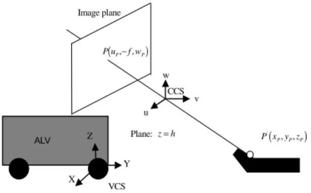
(4) r31 = cos φ sin ϕ , r32 = sin φ , r33 = cos φ cos ϕ ,. calculating the VCS coordinates of the ceiling lamp information, including the line segments and the corners, is similar to the method described above. In addition, the. and θ is the pan angle, φ the tilt angle, and ϕ the swing angle, of the camera with respect to the VCS; and. ( xd , y d , z d ). height between the floor and the ceiling is known in advance.. is the translation vector from the origin of. 4. Matching Features with Learned Model. the CCS to the origin of the VCS. The values of θ, φ, ϕ,. x d , y d , and z d are measured by performing camera. There are several existing algorithms for line-pattern and point-pattern matching. For example, the General-. calibration.. ized Hough Transform (GHT) is a popular approach to. 3.3. Locating Environment Features. arbitrary pattern matching. It also works for this study.. One selected environment feature is the baseline on. However, the GHT is time consuming. Thus it is desired. the building wall. On the abstract level, these visual fea-. to use a faster and simpler matching method for applica-. tures can be categorized into two classes, straight lines. tions. Another problem arises when computer vision in-. and corners of line segments. In this section, the geomet-. accuracy and image processing errors are involved. This. ric properties of the baseline, whose height is fixed and. makes perfect matching impossible, so a fault-tolerant. known in advance, are used to calculate the VCS coor-. matching algorithm is required. Furthermore, sometimes. dinates of the baseline segments detected in an input. the newly detected features in the local model may not. image. The method for calculating the VCS coordinates. exist in the learned global model, so the algorithm should. of a corner point, which is located on a baseline, is de-. also be capable of partial matching.. scribed in the following.. There is a basic assumption for the experimental en-. As shown in Figure3.3, the height of the baseline is. vironment: the objects, namely, the walls and doors, and. known in advance, after back-projecting a point P in the. the ceiling lamps, in the environment are all in two or-. image into the VCS, we can get P'.. thogonal directions. With this assumption, the environ-. Another type of selected environment feature comes. ment features can be treated as a set of orthogonal line. from the boundary information of ceiling lamps. Note. segments. In this study, we use two matching algorithms,. that just one set of parallel lines on the ceiling in the ac-. one for line-segment matching [8] and the other for cor-. quired image is utilized. The reason is that we view a. ner-matching [10] to meet the above three requirements.. ceiling lamp as a rectangle, so one set of parallel lines are enough to describe the characteristics of it. In this study, we select the left and the right boundaries of the. Image plane. ceiling lamp as our features. The way we employ for y. P(uP ,− f , wP ). x. w. VCS. CCS. ω. y'. ALV. v. u Plane: z = h. Z. ALV. P' ( x P , yP , zP ). (xp',y p'). Y. GCS. X. x'. Figure 3.2 The relation between 2D coordinate systems x-y and x'-y' represented by a translation vector (x ′p , y ′p ) and a rotation angle ω.. Figure 3.3. VCS. Configuration of the system for finding. the back-projection point for an image pixel..

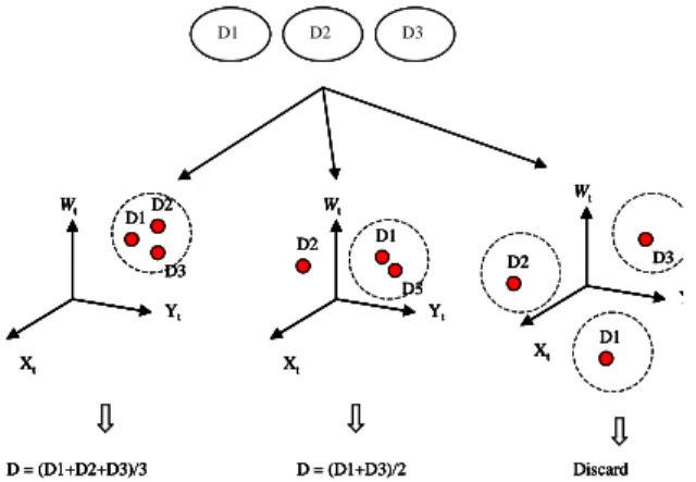
(5) 5. Side-View Model Learning. ALV location after performing the side-view model. The goal of the proposed model learning method in. learning procedure described in section 5. Ideally, all the. this study is to construct environment models from col-. three displacements must be identical. Unfortunately,. lected data automatically. Because of the inaccuracy of. because of image processing and vision computation. control actions, the estimated location of an ALV is not. errors, they might be different. This is undesirable.. very accurate. Correcting the position of ALV is a neces-. Therefore, we have to merge the model learning results. sary work for building an accurate environment model.. from the three cameras for building the top view of the. This can avoid error accumulation in a long learning. environment model. The data-fusion idea for generating. process. As shown in Figure 3.2, the ALV location is D1. described by the ALV slant angle ω and the ALV position. D2. D3. (x, y). We first correct the slant angle of the ALV. Then a model-matching approach is used to correct the position Wt. of the ALV. The learning procedure is described as fol-. D1. D2 D2. low.. Wt. Wt D1. D3. D2. D3 D3 Yt. Step 1. Set the initial global model as empty. Step 2. Extract environment features from the captured image.. Xt. Y. Yt Xt. Xt. D1. Step 3.Calculate the estimated position and orientation of the D = (D1+D2+D3)/3. ALV by the control data [12]. Calculate VCS coordinates of the extracted environment features. Step 4. Adjust the turn angle of the ALV by input features and re-compute ALV location. Step 5. Calculate the GCS of the detected environment features by the re-computed ALV location. Step 6. Set up a local model by collecting the data of the local features computed in Step 6.. D = (D1+D3)/2. Discard. Figure 6.1 Decide a universal position vector. the environment model using the learning result from the multiple data is shown in Figure 6.1. In each learning cycle, three sets of image data are collected, and each yields a position vector (xt, yt, ω) for computing an accurate ALV location after performing the matching step in the side-view model learning procedure.. Step 7. If the global model is non-empty, match the local model. The three displacements, D1, D2, and D3, presumable. with the global model by using the line-segment or cor-. should be identical. But due to image processing and. ner-matching scheme; else, go to Step 10.. vision computation errors, they might be different, and it. Step 8. Recalculate the accurate ALV location. Then recalculate. is undesirable. We propose here a method to decide the. the accurate position of the local features by the match-. single displacement, D, from the multiple-view data for. ing result and the recalculated ALV location.. use in all the three side views (the two corridor sides and. Step 9. Attach the local model to the global model.. the corridor ceiling). The distance “Dis” between two. Step 10. Repeat Steps 2 through 10 for the next learning cycle.. position vectors, (x1, y1, ω1) and (x2, y2, ω1), is defined as following.. 6. Data Fusion for Generating Overall Environment Model. Dis =. (x1 − x2 )2 + ( y1 − y2 )2 + (ω1 − ω 2 )2. As shown in Figure 6.1, if any two displacements of 6.1. Generating Environment Model Using Multiple. the three are separated by a distance which is smaller. Image. than a pre-selected value T, then we decide that the three. At each model learning cycle, there are three sets of. position vectors are similar enough. Then, we use their. independent image data grabbed from the three cameras. average as the desired single position vector. If two of. at the same instance. From each image data, there yields. these displacements whose distance is closed enough (<T). a position vector (xt, yt, ω) for computing an accurate. and the third one is far away from the two, then we use.

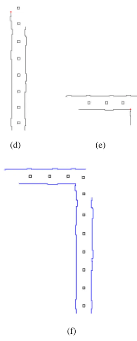
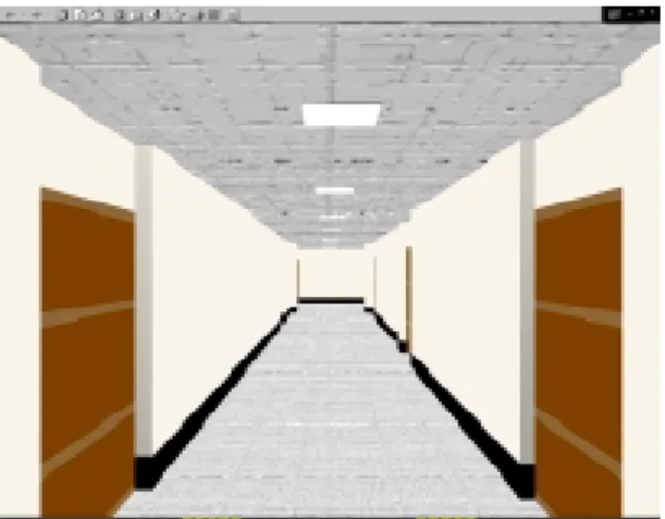
(6) the average of the two similar position vectors as the. The final step of this study is to process 3-D data. desired vector. Otherwise, if the three position vectors. building a VR environment model. The result is com-. are all mutually dissimilar, i.e., if the distance between. posed of a set of planar surfaces, represented as polygons,. any two of them is larger than a pre-selected value T,. in 3-D space. These polygons are defined using the vir-. then we discard all of them, ignore the result of this. tual reality markup language (VRML). To view a VRML. learning cycle, and go to the next learning cycle.. document, a plug-in application should be installed to the. 6.2. Restoration of 2-D Environment Model. browser. This plug-in application allow users to access. As shown in Figure 6.2, some features cannot be. VRML worlds with their current browser technologies.. modeled accurately by the ALV because of the limit. Our program will generate VRML document automati-. viewed of the cameras. In the example, each corner is. cally depending on the 3-D environment data acquired. marked by a small black spot, and each unseen feature is. by the method described in section 6. The result can be. marked by a dash line. The ALV cannot observe the cor-. used for various applications such as ALV navigation,. ner C, and the two neighboring lines of C are also hidden. exhibit houses on world wild web, in which users can. partially. Therefore, restoring these unseen features is. have a better feeling of involvement in the VR environ-. necessary to make the acquired 2-D environment model. ment.. more completely.. 8. Experimental Results The experiments of ALV model learning and 3-D VR environment reconstruction were performed in the corridor of a building in National Chiao Tung University. Figure 6.2: An example of senses out of sight. 6.3. Merge of Data of Distinct Corridor Sections. Figure 8.1(a) shows a top view of real corridor data acquired by the model learning scheme. Figure 8.2 (b) shows restoration of a corridor data of Figure 8.1(b).. If more than one corridor exists in the indoor envi-. Figure 8.2 is an illustrative example of corridor section. ronment, or more specifically if there exist crossings in. merging. The corresponding points of the two corridors. the environment, the proposed method, which performs. are drawn with points. Figure 8.3 is a complete model of. model learning for each corridor separately, is insuffi-. Figure 8.2(f). Figure 8.4 and Figure 8.5 shows a result of. cient. Instead, merging of data of distinct corridor sec-. 3-D indoor VR model reconstruction of Figure 8.3.. tions is necessary for constructing a complete environment model. An assumption made in this study is that for. 9. Conclusions. any two neighboring corridor sections there must exist a certain overlapping area. This assumption is reasonable. In this paper, we have proposed a system for learning. because data collection is involved by human beings.. environment models and reconstructing corresponding. After traveling through the entire environment, the rela-. 3-D VR models by ALV navigation and computer vision. tion between two corridors is known. To merge the two. techniques. Certain assumptions about the scene struc-. sections, we can find the corresponding points of the two. ture are utilized to reduce the complexity of the system.. corridors. Using the relation between two corresponding. The system not only collects the information of the en-. points, we can merge two distinct corridor sections.. vironment features to build up a top-view environment model but also reconstructs a corresponding 3-D VR. 7. Construction of 3-D Indoor VR Environment Model. environment model by performing some post-processing works to the observed 3-D data. For environment learning, an algorithm for orthogonal-line-segment and cor-.

(7) ner-pattern matching and a systematical algorithm for constructing. the. learned. environment. model. by. multi-camera image data fusion have been utilized to improve the system performance. Because of the limit of the camera view and defective matching results, a scheme for restoring the observed 3-D data has also been proposed. Furthermore, a scheme to reconstruct 3-D VR environment models by using the virtual reality markup language (VRML) has been proposed. The proposed. (d). (e). learning and reconstruction system has been implemented on a prototype ALV. Successful reconstruction of 3-D VR environment models in indoor corridor environments confirms the feasibility of the proposed approach.. (f) Figure 8.2 An illustrative example of corridor section merging. (a) One corridor model. (b) A neighboring corridor model of (a). (c) Translate view point of (b). (d) and (e) Corresponding point in (a) and (c). (f) Result of merge. Figure 8.1: An example of restoration of a corridor in real environment. (a) Before restoration. (b) After restoration. The corners are marked by a small black spot.. (a). (b) Figure 8.3 A complete model of Figure 8.2(f) which is the result of restoration. The border line are added to made the model more complete (c).

(8) Takeshi Shakunaga“3-D Corridor Scene Modeling from a Single View under Natural Lighting Conditions” IEEE Transactions on Pattern Analysis and machine intelligence, Vol. 14, No. 2, pp. 293-298, February 1992. [7] Shadia Elgazzar, Ramiro Lisscano, François Blais, and Andrew Miles,“ Active Range Sensing for Indoor Environment Modeling”, IEEE Transactions on Instrumentation and Measurement, Vol. 47, No. 1, pp. 260-264, February 1998. [8] F. M. Pan and W. H. Tsai,“Automatic environment learning and path generation for indoor autonomous land vehicle guidance using computer vision techniques”, Proc. of 1993 National Computer Symposium, Chia-Yi, Taiwan, Republic of China, pp. 311-321, 1993. [9] Guan-Yu Chen and W. H. Tsai, “ An Incremental-Learning-by-Navigation Approach to Vision-Based Autonomous Land Vehicle Guidance in Indoor Environments Using Vertical Line Information and Multi-Weighted Generalized Hough Transform Technique ” , IEEE Transaction on System, Man and Cybernetics-Part B: Cybernetics, Vol. 28, No. 5,pp. 740-748, October 1998. [10] Guan-Yu and W. H. Tsai, “A New approach to vision-based unsupervised learning of unexplored indoor environment for autonomous land vehicle navigation”, Robotics and Computer Integrated Manufacturing 15 (1999) pp. 353-364. [11] Zhi-Fang Yang and W. H. Tsai,“Viewing Corridors as Right Parallelepipeds for Vision-Based Vehicle Location”, IEEE Transactions on Industrial Electronics, Vol. 46, No. 3, June 1999. [12] P. Y. Ku and W. H. Tsai,“Model-based guidance of autonomous land vehicle for indoor navigation”, Proceedings of Workshop on Computer Vision, Graphics and Image Processing, Taipei, Taiwan, Republic of China, pp 165-174, Aug. 1989.. [6]. Fig. 8-4 The reconstructed 3D-VR Model.. Figure 8.5: 3-D VR model of Figure 8.4 from different viewpoint.. References [1]. [2]. [3]. [4]. [5]. J. Illingworth and A. Hiton, “Looking to build a model world: automatic construction of static object models using computer vision,” Journal of Electronics& Communication Engineering, June 1998. X. Lebègue and J. K. Aggarwal, “Extraction and Interpretation of Semantically Significant Line Segments for a Mobile Robot,” Proc. of 1992 IEEE Intl. Conf. on Robotics and Automation, Nice, France, pp. 1778-1785, May 1992. X. Lebègue and J. K. Aggarwal, “Significant Line Segments for an Indoor Mobile Robot,” Proc. of 1993 IEEE Transactions on Robotics and Automation. Vol. 9, No. 6, pp 801-815, December 1993. X. Lebègue and J. K. Aggarwal, “Generation of Architectural CAD Models Using a Mobile Robot,” Proc. of 1994 IEEE Intl. Conf. on Robotics and Automation, San Diego, California, U.S.A., Vol. 1, pp. 711-717, May 1994. X. Lebègue and J. K. Aggarwal, “Automatic Creation of Architectural CAD models,” CAD-Based Vision Workshop, 1994., Proceedings of the 1994 Second, page(s) 82-89..

(9)