國
立
交
通
大
學
統計學研究所
博
士
論
文
最高密度顯著性檢定
Highest Density Significance Test
研究生:陳弘家
指導教授:陳鄰安教授
中 華 民 國 九 十 六 年 六 月
最高密度顯著性檢定
Highest Density Significance Test
研 究 生:陳弘家 Student:Hung-Chia Chen
指導教授:陳鄰安 Advisor:Lin-An Chen
國 立 交 通 大 學
統 計 學 研 究 所
博 士 論 文
A ThesisSubmitted to Institute of Statistics College of Science
National Chiao Tung University in partial Fulfillment of the Requirements
for the Degree of Ph. D. in Statistics June 2007 Hsinchu, Taiwan
中華民國九十六年六月
最高密度顯著性檢定
學生:陳弘家
指導教授:陳鄰安
國立交通大學統計學研究所 博士班
中文摘要
顯著性檢定是一種藉由計算p值的方法,用於衡量是否違反虛無假設的統計 證據,傳統的顯著性檢定選擇一個統計量T = t(X),同時決定一個極端的集合, 此集合包含比觀測值 t(x0)極端或相當的所有點。但是,這個方法有可能無法找 到一個合適的統計量,或者不存在一個普遍性的最佳性質來支持既存的顯著性檢 定。因此,我們提出一個新的顯著性檢定,設定極端集合包含所有發生機率比觀 測值x0機率小的點,稱為最高密度顯著性(HDS)檢定。此方法應用到較小的機率 顯示存在更強的證據否定虛無假設的概念,且將一個樣本X藉由機率比分為極端 與非極端的兩個集合。在相同的p值檢定中,我們發現HDS檢定的非極端集合體 積最小,此為一最佳性質。我們更進一步延伸HDS檢定來建立控制圖,同時監控 所有的參數,並且能精準的達到第一類誤差的機率。藉由監控樣本點的機率來辨 識是否受到控制,不像傳統的控制圖是依據樣本平均和全距來監控。 關鍵詞:控制圖,最高密定顯著性檢定,p 值,最小體積Highest Density Significance Test
student:Hung-Chia Chen
Advisor:Dr. Lin-An Chen
Institute of Staistics
National Chiao Tung University
Abstract
The significance test is a method for measuring statistical evidence against null hypothesis H0 by computing p-value. The classical significance test chooses a test
statistic T = t(X) and determines the extreme set representing the sample set with values t(x) greater than or equal to t(x0), where x0 is the observed sample. It may be
difficult to choose a suitable test statistic for the test, or there is no generally accepted optimal theory to support the existed significance tests. Now, we propose a new significance test, called the highest density significance (HDS) test, setting extreme set including those sample points with probabilities less than or equal to it of x0. It
applies the concept that the smaller probability of an observation X = x0 reveals
stronger evidence of departure from H0. This test virtually classifies the sample space
of random sample X into extreme set and the non-extreme set through a concept of probability ratio. We also show that this test shares an optimal property for that it has smallest volume among the class of non-extreme sets of significance tests with the same p-value. Further, we extend HDS test to set up a control chart which can monitor all the parameters simultaneously and the probability of type I error is precisely attained. Unlike the classical control charts that track statistics such as sample mean X or sample range R, it is tracking the density value of the sample point to classify if it is in control.
Contents
1 Introduction 1
1.1 Point Estimation . . . 2
1.2 Hypothesis Testing . . . 3
1.2.1 Neyman-Pearson Formulation . . . 4
1.2.2 Significance Hypothesis Test . . . 4
1.3 Interval Estimation . . . 6
1.4 Control Chart . . . 7
1.5 Summary . . . 7
2 Probability and Plausibility 9 2.1 Concepts of Probability and Plausibility . . . 9
2.2 Probability and Plausibility Principles . . . 15
3 Highest Density Significance Test 19 3.1 Definition and Properties . . . 20
3.1.1 Likelihood-Based Significance Test . . . 20
3.1.2 Smallest Volume Non-Extreme Set significance Test . . . 22
3.2 HDS Test for Continuous Distributions . . . 24
3.3 HDS Test for Discrete Distributions . . . 28
3.4 The Best Significance Tests . . . 33
3.5 Some Further Developments of HDS Test . . . 39
3.5.1 Approximate HDS Test . . . 39
4 Control Charts 49 4.1 Density Control Charts . . . 50 4.2 Density Control Charts for Some Distributions . . . 52 4.2.1 Density Control Charts for Normal Distribution . . . 52 4.2.2 Density Control Charts for Negative Exponential Distribution . . . . 60 4.3 Approximate Density Control Charts . . . 66 4.3.1 Approximate Binomial Density Control Charts . . . 68 4.3.2 Approximate Gamma Density Control Charts . . . 69
5 Future Study 71
5.1 Nuisance Parameters . . . 71 5.2 Significance Test for Hypothesis of Distribution Function . . . 71 5.3 Incomplete Data . . . 72
Appendix: p-values for Binomial HDS Test 74
List of Figures
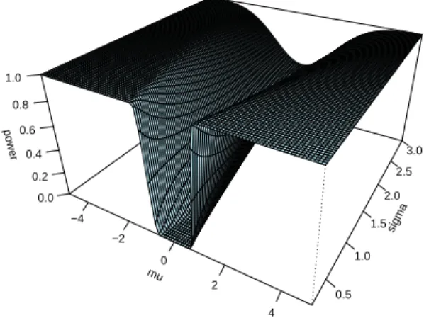
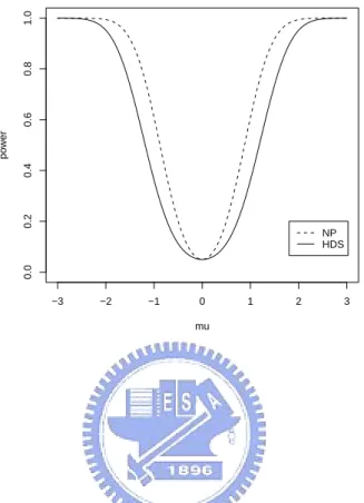
1 Power of HDS test and n=5 . . . . 44
2 Power of Neyman-Pearson test and n=5 . . . . 44
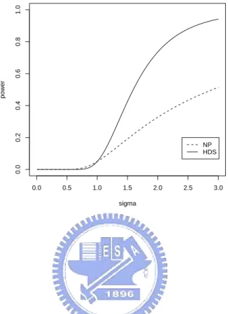
3 Powers of the two tests as σ2 = 1 and n=5 . . . . 45
4 Powers of the two tests as σ2 = 2 and n=5 . . . . 45
5 Powers of the two tests as σ2 = 3 and n=5 . . . . 46
6 Powers of the two tests as σ2 = 0.5 and n=5 . . . . 46
7 Powers of the two tests as µ = 0 and n=5 . . . . 47
8 Powers of the two tests as µ = 1 and n=5 . . . . 47
9 X chart for Vane Opening . . . .¯ 54
10 R chart for Vane Opening . . . . 54
11 X chart for Vane Opening,revised limits . . . .¯ 55
12 R chart for Vane Opening, revised limit . . . . 55
13 Log-density control chart for Vane Opening . . . 56
14 Log-density control chart for Vane Opening, revised limits . . . 57
15 Log-density control chart for Vane Opening, twice revised limits . . . 58
16 A control parabola for normal distribution. . . 59
17 Parabola control chart for vane opening . . . 60
18 Log-density control chart for Particle Count . . . 64
19 Log-density control chart for Particle Count, revised limit . . . 64
20 χ2 control chart for negative exponential distribution. . . . 65
List of Tables
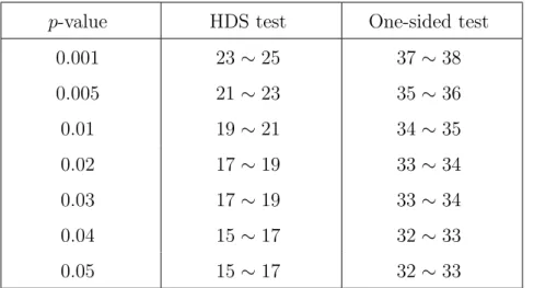
1 Numbers of non-extreme points for HDS test and one-sided Fisherian
signifi-cance test with approximated equal p-value. . . . 31
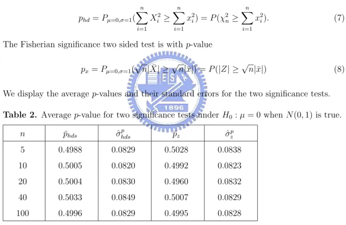
2 Average p-value for two significance tests under H0 : µ = 0 when N(0, 1) is true. . . 36
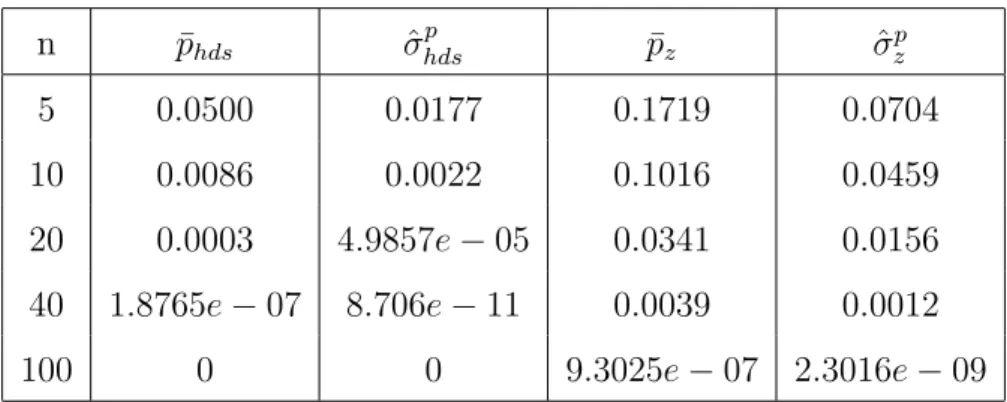
3 Average p-value for two significance tests under H0 : µ = 0 when N(0, 4) is true. . . 37
4 Average p-value for two significance tests under H0 : µ = 1 when N(0, 4) is true. . . 38
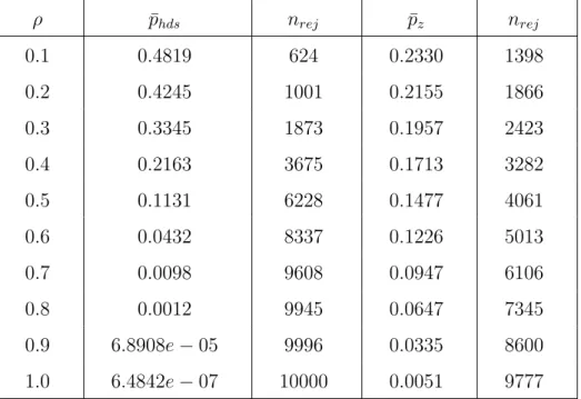
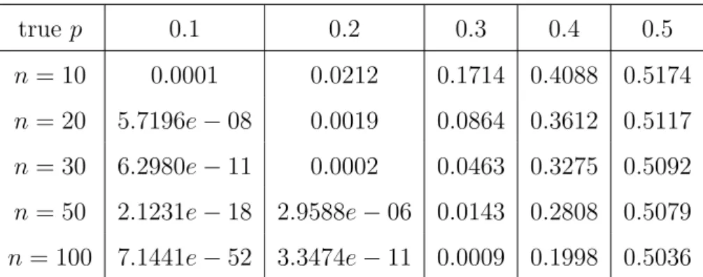
5 Average p-value for two significance tests under H0 : µ = 0 when AR(1) is true. 39 6 p-value of approximate HDS test for binomial distribution under H0 : p = 0.5. 41 7 Approximate HDS test for Cauchy sample when null hypothesis is true. . . . 42
8 Approximate HDS test for Cauchy sample when µ = 1. . . . 42
9 ARL for the mean and location shifts. . . 62
10 Lower control limit and sample values of the test statistic function. . . 63
11 ARLexact ARLappro for normal distribution (n = 5). . . . 68
A.1 p-value for binomial distribution under H0 : p = 0.5 (n = 2, ..., 5). . . . 74
A.2 p-value for binomial distribution under H0 : p = 0.5 (n = 6, ..., 10). . . . 74
A.3 p-value for binomial distribution under H0 : p = 0.5 (n = 11, ..., 15). . . . 74
A.4 p-value for binomial distribution under H0 : p = 0.5 (n = 16, ..., 20). . . . 75
A.5 p-value for binomial distribution under H0 : p = 0.5 (n = 21, ..., 25). . . . 75
1
Introduction
With great application in numerous different fields such as natural science, social science, or some others, statistics is frequently used to interpret characteristics of some phenom-ena involving randomness and variability. It plays a key role in information extraction and drawing conclusions for characteristics of the phenomena when a data set is collected from ex-periments or field studies. Information extraction includes data reduction and summarizing statistics from the raw data. Statistics not only analyze the observed data from experiments, but also assists designing the experiments. Prior to analysis of statistics, the practitioners or scientists should establish a statistical model that describes the data generation mechanism, and this is for developing statistical methods to condense the information for further making statistical inferences.
The simplest generic form of a statistical model, which was formulated by Fisher and may be seen in Azzalini(1996) and Spanos(1999), contains a probability model and a sampling model, and it purports to describe the population and its variation for data reduction. The probability model represents a probability space assigning a probability distribution Pθ on S where θ ∈ Θ is parameter point and S is the sample space. The sampling model is
viewed as the realization of the probability model or events drawn from the population. A generalized statement of statistical model including regression related models may be seen in McCullagh(2002) which is extended from Spanos(1999). Generally, the true parameter
θ of the probability model is usually unknown, but the parameters or the distributional
characteristics may be drawn conclusions from the observed data via statistical approaches. The efficiency of a statistical approach relies on the amount and appropriateness of the information being captured from the data. For specific, in-appropriateness of choosing sta-tistical model will never collect full information for stasta-tistical inferences. On the other hand, with a specified statistical model, various principles of information extraction resulted in var-ious information sets. Then the usefulness of the information will depend on the preferences of the practitioners or scientists for model and principle selection. The fact of statistical inferences in the literature, point estimation and Neyman-Pearson framework of hypothesis testing are solved respectively with solutions supporting with some desirable optimal prop-erties. However, as interpreted in Birnbaum(1962) “method such as significance tests and
interval estimates are in wide standard use for the purposes of reporting and interpreting the essential features of statistical evidence.” These two important statistical inference
prob-lems are not solved with solutions supported with desirable properties( Detailed description of these points will be stated latter).
Eventually, the practitioners or scientists would pay attention on what they should do, what they should believe, or what the data does tell, and all of these problems depend on the assumed statistical models and the ways of the data collection. Each specific inference problem require a specific amount of information, i.e., there is no principle that provides amount of information enough for every inference problem. For significance test problem, we will study what an amount of information is appropriate and how it does to reveal a desirable optimal property. Before to do this, we will review statistical inference problems. The following sections will contain three categories which are the most parts of statistical inference, point estimation, interval estimation and hypothesis test in statistical inference.
1.1
Point Estimation
Point estimation tries to present a value based on the observation to estimate the unknown parameter (or distributional characteristics) which often represents a location point or scale for the distribution. In point estimation with a mass data set, data reduction helps in information condensation that help practitioners summarizing useful statistics. When a summarized statistic is used for estimation of the unknown parameter, it is called an esti-mator of θ. Although computational easiness and naivety often be factors for data reduction to the practitioners, however, estimators developed from these considerations may not be efficient for statistical inferences.
With a great effort for efficient estimation technique, there are many approaches proposed for point estimation, for examples, the method of moments, maximum likelihood estimator, Bayes estimators, or EM algorithm, etc. For selection of estimators, criterions for evaluating estimators have also been proposed in literature. Some important ones are mean squared error, best unbiased, equivariance, average risk optimality, minimaxity, admissibility and asymptotic optimality (see Lehmann and Casella(1999) or Casella and Berger(2001)). In the literature, it has been done in deriving estimators supported with optimal properties
such as the uniformly minimum variance unbiased estimator, uniformly most powerful test, Bayes estimator etc. With this achievement, we will not spend any effort on point estimation to seek for any other optimality. However, the maximum likelihood estimator does provide interesting information in the statistical model that is helpful for other statistical inference problems.
For technique with asymptotic optimality, a widely adopted estimator in the parametric model is maximum likelihood estimator which can be traced back to Fisher(1912, 1922a, 1922b, 1925a, 1925b, 1935). The maximum likelihood estimator is derived from solving a parameter point with highest likelihood. It represents the most likely value in the parameter space for which a sample point has already occurred. The use of most likely value leads the maximum likelihood estimator to be not only consistent but also efficient. Besides from estimation for estimators, the Fisher information revealed in the efficiency of the maximum likelihood estimator has been applied in construction of other inference techniques such as the score test and Wald’s test. This concept of most likely values may also be interesting for some unsolved statistical inference problems.
1.2
Hypothesis Testing
In the topic of hypothesis testing, there are two important categories for hypothesis speci-fication, the significance test and the Neyman-Pearson formulation. The Neyman-Pearson formulation considers a decision problem which is composed by two components, null hy-pothesis and alternative hyhy-pothesis. On the other hand, the significance test considers only one hypothesis, the null hypothesis H0. The significance test may occurs that H0 is drawn
from scientific guess and we have no idea on assumption about alternative hypothesis when the null hypothesis is not true. Another case is that the model is developed to be checked with new data by a selection process on a subset when H0 is true. Then the problem for
significance test is more general than the Neyman-Pearson formulation in that when H0 is
1.2.1 Neyman-Pearson Formulation
The hypothesis testing for Neyman-Pearson formulation considering a null hypothesis H0and
an alternative hypothesis H1 is different from significance test which considers only the null
hypothesis. The theory of Neyman-Pearson lemma applies the ratio of the likelihoods with one that H0is true and one that H1is true. This leads to the result of most powerful test when H0 and H1 are both simple and uniformly most powerful test for some composite hypotheses
and some specific distributions. Hacking(1965) interpreted the the law of likelihood in the following:
If one hypothesis, H1, implies that a random variable X taking the value x with
prob-ability is f1(x), while another hypothesis, H2, implies that the probability is f2(x),
then the observation X=x is evidence supporting H1 over H2 if f1(x) > f2(x), and the
likelihood ratio, f1(x)/f2(x), measures the strength of the evidence.
The law of likelihood gathers the information of likelihoods for that H0 and H1 are true and
use the likelihood ratio to help statisticians in drawing conclusion of acceptance or rejection of null hypothesis.
Besides that it has been with derived optimality, the Neyman-Pearson hypothesis testing can be solved with sample size determination to have a desired power. The significance test is not available in justifying the sample size for the fact that anything is possible when H0 is
not true. There is one other advantage for the Neyman-Pearson hypothesis testing. The use of likelihood ratio will automatically derive the test statistic. This desired property is not shared with most other hypothsis testing problems. With the interesting results including the optimal property, samples size determination and test statistic derivation, the theory of Neyman-Pearson lemma provides us a desired test when an alternative hypothesis may be specified. However, in many practical situations, to specify an alternative hypothesis is not appropriate. In this case, what can we do?
1.2.2 Significance Hypothesis Test
For developing more than 200 years, the significance test has been popularly used in many branches of applied science. Some earlier applications of significance test include Armitage’s
(1983) claim finding the germ of the idea in a medical discussion from 1662 and Arbuth-not’s(1710) observation that the male births exceeds the female births. Some important significance tests developed latter include the Karl Pearson’s(1900) χ2 test and W.S.
Gos-set’s (1908) student test , the first small-sample test. Significance tests were given their modern justification and then popularized by Fisher who derived most of the test statistics that were broadly adopted in a series of papers and books during 1920s and 1930s. Tradi-tionally, a significance test is to examine whether a given data is in concordance with H0.
The practitioners generally formulate a null hypothesis of interest and specify a test statistic to interpret if the observation provides evidence against H0. Then, the p-value is determined
as the probability of the sample set for that the test statistic is at least as extreme as its observed value when H0 is true:
p = P r(T at least as extreme as the value observed |H0).,
where T represents the test statistic.
A significance test always drawn conclusion in terms of p-value. It interprets the p-value as evidence for that the data is consistent with the null hypothesis by concluding that the hypothesis is significant or not to be true. This is different from the Neyman-Pearson framework which always draws conclusion of acceptance or rejection of null hypothesis. The significance test is often being criticized for that it is hard to provide acceptable reason in supporting the chosen test statistic although the sufficient statistic is usually recommended. There is other way in the interpretation of the p-value by saying that it represents the strength of evidence against null hypothesis. From this point, the extreme set has to contain sample points which are at least as large as the observed value or absolute value of the test statistic (see this point in Schervish(1996) and Sackrowitz and Samuuel-Chan (1999))
Schervish(1996), Royall(1997) and Donahue(1999) argued that the typical p-value couldn’t completely interpret the statistical evidence. With this concern, the p-value has been re-defined as the probability of the extreme points determined by the joint density function. In the empirical studies, Hung et al.(1997), and Donahue(1999) proposed modifications for significance test based on the Neyman-Pearson approach where two hypotheses are assumed. They discussed p-value in the class of Neyman-Pearson formulation regardless of no
alter-native assumption. In other words, they connect the Neyman-Pearson formulation to the significance test. This argument is different from the approach that we will introduce.
It is known that the likelihood function has been recognized as a mathematical represen-tation of the evidence (Birnbaum 1962). However, without consistent technique to defining evidence, the classical approaches for the discipline of the significance test really make users confused for that the hypothesis may be significant for one test statistic and insignificant for the other one. Thus, there needs one approach to interpret the statistical evidence that is more convincing than the existing approaches. Hopefully there are interesting properties for this new approach.
1.3
Interval Estimation
Point estimation is always criticized for reporting only a single value for the unknown param-eter to the practitioners without flexibility presenting the description of variability. There are two techniques to overcome this drawback. One is a range or interval containing the parameter that contains a specified level of probability or confidence. The other one is hy-pothesis testing which provides a tool with decision, either determining to reject or accept
H0 or reporting a p-value.
The techniques of interval estimation are always with close relation to them for point estimation and hypothesis test. The interval with confidence level 1 − α may be derived from the inversion of a level 1−α acceptance region of hypothesis testing. Interval estimation may also be derived from which Bayesian approaches which one is criticized for the reason of its determination of subjectively prior distribution. Mood (1974) also categorized the methods of parametric interval estimation into two main techniques. One is based on the pivotal-quantity, and the other is based on the statistical method. Statistical method constructs the confidence interval from the distribution of a statistic. The pivotal-quantity method is the most popular one to derive the confidence interval. But, it requires the existence of a pivotal quantity. However, the pivotal quantity is frequently absent. When this happens, the alternative methods would be the statistical method or the inversion of hypothesis test. Most of the methods stated above are connected with point estimation. They consider the interval as a set composed by two points involving parameters, and they estimate the two
points via point estimation.
Without using point estimation, Hyndman (1996) proposed the highest density regions consisting of parameter points of relatively high density due as the confidence set for the parameters. Formulated from likelihood function, the highest density region has the property of smallest volume in sample space which will be discussed in latter section.
1.4
Control Chart
The control charts in Statistical Process Control (SPC) are useful tools to monitor whether various production processes in industry are in statistical control or not. A process is in statistical control when the probability distribution of a random variable which represents the characteristic of the process is unchanged in time. It is often that the distribution involves several parameters. The general way to treat this process is to construct a control chart for each parameter,for example, the ¯X and R charts. As we have done for a process
with several characteristics(values), the most popular way to monitor the process is to draw conclusion through the results from several control charts.
According to the fact that conclusion from a combination of control charts for variables, it may lead to incorrect control (probability) limits. This drawback has been received extensive attention in literature (Mason, et al. (1997) and Wierda (1994)). Incorrect control limits happen not only in a multivariate variable case but also in the case of univariate variable with distribution involving several parameters. Why not we construct a control chart to assure that the control limits are correct for this circumstance? This problem is similar to test several hypotheses simultaneously. Hence we could consider all of them in a single hypothesis which could interpret if a process is in statistical control.
1.5
Summary
Started from introducing of statistical model, we reviewed the statistical inference approaches in previous sections. The approach with techniques based on likelihood function is espe-cially interesting. The use of maximum likelihood estimation leads to the desired property of asymptotically attaining Cramer-Rao lower bound. On the other hand, the use of
likeli-hood ratio results the most power test. In the following sections, we will study a point in statistical inference that is somehow different from the sufficiency and conditionality. We will investigate the information that is contained in the statistical model and introduce two statistical principles. Then we will follow these principles to define a new extreme set and conduct a new significance hypothesis test, highest density significance test, in section 3 and 4. Further, we will develop several different control charts for different distributions in section 5.
2
Probability and Plausibility
2.1
Concepts of Probability and Plausibility
Birnbaum(1962) proposed that “report of experimental results in scientific journals should
in principle be descriptions of likelihood functions, when adequate mathematical-statistical models can be assumed, rather than reports of significance levels or interval estimates.” The
likelihood function formulated from statistical model has been broadly applied with a long history in statistical inference. The simplest form of the statistical model is the case that there existed a random sample X1, ..., Xn drawn from a distribution with pdf f (x, θ), x ∈ Rx, θ ∈ Θ where Rx is sample space of variable X and Θ is the parameter space.
Most statistical inference problems in parametric model arise from the fact that we do not know the true parameter θ as we have the observations. According to the occurrence of the observation, we wish to infer something requested from problems concerning about the true parameter. For dealing with the raised statistical problem, we generally want to summarize important and necessary information to develop a statistical procedure with desired property. Among many available procedures, we expect a desired one to achieve the followings: (a) Generally accepted criterion of optimal procedures.
(b) Demonstrate that the best procedure is possible, i.e. the best one is obtainable.
Various statistical problems need various amount of information to accomplish the achieve-ment. For a general study, it is interesting to observe that the total amount information is contained in the statistical model postulated by Fisher as
Γx = {f (x, θ)x ∈ Rx, θ ∈ Θ, X = (X1, ..., Xn) is a random sample}. (1)
For aiming in solving various statistical problems, there are several techniques implemented for data reduction, which are proposed trying to gather possible information for inference of θ. With disciplines of statistical problem, it has not been known if there is a technique of data reduction that may accomplish our goal for dealing with various statistical inference problems. The reason raising this question is related to the concept of the sufficiency which was introduced by Fisher(1922). This concept is now played a central role in frequency based inferences and then many frequentist approaches are recommended to rely on the
sufficient statistic. It is general in literature that we define a statistic S(X) to be sufficient for the family {f (x, θ), θ ∈ Θ} if the conditional distribution of the random sample X given a value of S(X) does not depend on θ (see, for example Spanos (1999, p627)). Suppose that the sufficient statistic provides enough information for dealing with all statistical inference problems. We must see that there is a statistical technique involving sufficient statistic for every inference problem is shown to have some desirable properties. However, this is not true in some important statistical inference problems.
Sufficient statistic perhaps plays the most important part in developing minimum variance unbiased estimator. Let’s see its role in some other statistical inference problems. Mainly due to Barnard (1949,1980), the pivotal quantity, an elegant technique, has been very popularly applied for constructing the confidence interval. On the other hand, a significance test, formulated by Fisher (1915), is a method for measuring statistical evidence against a null hypothesis H0 and is done by selecting a test statistic T and computing the probability
of the tail area of the distribution of T beyond its observed value which is called the p-value. The pivotal quantity for confidence interval and the test statistic for significance test are generally recommended to be constructed involving the sufficient statistic without any careful justification. Unfortunately, the statistical procedures based on them are not justified with any desired optimal properties. It may be that the sufficient statistic, especially the minimal one, condenses the information in the statistical model Γx so much that it is not
appropriate to be applied to all statistical problems.
Vapnik (1998, p12) argued the techniques for problems in statistical inferences that a restricted amount of information only can solve some special problems and it can never solve all different statistical problems with effective procedures. In interval estimation and significance test, the lack of optimal properties reveals that there must have interesting evidence that can’t be discovered in a sufficient statistic. Silvey (1975) and Lindsey (1996) both pointed out that many frequentist theory and techniques for confidence sets appear ad hoc because they are not wholly model-based, relying on the likelihood function, and other single unified principle. It is lack a technique that can capture useful information embedded in the data and the model for construction of inference methods.
Without applying the likelihood function, the techniques for confidence interval in liter-ature are not convincing in terms of plausibility which has the information represented by
the size of the likelihood function L(θ, x) when X = x is observed. This indicates that we should be careful in using sufficient statistic to construct confidence interval. The problem raised by Silvey(1975) and Lindsey(1996) also occurs in the significance test problem. With assuming that H0 is true, the existed significance tests do not restrict the set of probable
non-extreme points. This results that the p-values computed from these significant tests not appropriate as evidence against H0.
Let’s examine the concern of Silvey (1975) and Lindsey (1996) about plausibility and probability of sufficient-statistic based on confidence interval and significance test. When vector X = x is observed , we say that θ1 is more plausible than θ2 if L(x, θ1) > L(x, θ2),
where L(θ, x) is the likelihood function for random sample X. Regarding to the null hy-pothesis H0 : θ = θ0, we may say that sample point x1 is more probable than another point x2 if L(x1, θ) > L(x2, θ). Suppose that C(X) is a 100(1 − α)% confidence interval for θ and A(x0) is the non-extreme set for a significance test. The likelihood sets corresponding with
confidence interval C(X) and significance test when X = x0 is observed are, respectively, LSC = {L(θ, x) : θ ∈ C(x), x ∈ Rnx} for confidence interval, and
LSA(x0) = {L(θ0, x) : x ∈ A(x0)} for significance test.
For interval estimation, the likelihood set is set of plausibilities values for a confidence interval. As we have discussed above, a set to be more plausibility may be more suitable to play as a confidence interval or significance test. Thus we have to choose a confidence set whose corresponding likelihood set stay away from zero. On the other words, we want to construct a confidence interval which includes the most plausible points. The likelihood sets of some typical confidence intervals will be shown in the following examples.
Example 2.1. Let X1, ..., Xn be a random sample drawn from the normal distribution N(µ, σ2). First we consider the confidence interval for mean µ with known variance σ = 1
for convenience, and then the sample space is Rx = R. The popularly used 100(1 − α)%
confidence interval based on sufficient statistic ¯X for µ is
( ¯X − zα/2 1 √ n, ¯X + zα/2 1 √ n).
Three facts are employed in deriving the likelihood set. (1). ¯x − zα/2√1n ≤ µ ≤ ¯x + zα/2√1n
if and only if n(¯x − µ)2 ≤ z2
α/2. (2). n
P
i=1
(0, ∞). (3). ¯X and Pn i=1
(Xi− ¯X)2 ∼ χ2(n − 1) are independent. The following we derive its
corresponding likelihood set.
LSC = {(2π)1n/2e− n P i=1(xi−µ) 2 2 : µ ∈ (¯x − zα/2√1 n, ¯x + zα/2√1n), x1 ... xn ∈ R n} = { 1 (2π)n/2e −1 2( n P i=1 (xi−¯x)2+n(¯x−µ)2) : µ ∈ (¯x − zα/2√1n, ¯x + zα/2√1n), x1 ... xn ∈ R n} = { 1 (2π)n/2e− 1 2(y1+y2): 0 ≤ y2 ≤ z2 α/2, 0 < y1 < ∞} = { 1 (2π)n/2e− 1 2y : 0 ≤ y < ∞} = 1 (2π)n/2(0, 1].
In this example, it has been shown that the likelihood set includes zero which indicates that this confidence interval is implausible.
Similarly, the popularly used significance test based on sufficient statistic Pn
i=1
Xi when X = x0 is to compute p-value P (
√
n| ¯X| ≥√n|¯x0||µ = 0) where µ = 0 representing that H0
is true. By denoting ¯x0 as the sample mean of vector x0, the likelihood set of the significance
test derived in the following
LSA(x0) = { 1 (2π)n/2e− n P i=1 x2i 2 : |¯x| ≤ |¯x0|, x1 ... xn ∈ R n} = { 1 (2π)n/2e −1 2( n P i=1 (xi−¯x)2+n¯x2) : |¯x| ≤ |¯x0|, x1 ... xn ∈ R n} = LSC.
is identical to it for the confidence interval for mean.
Next, we consider the confidence interval for variance σ2 where µ = µ
0 is also assumed
to be known. With sufficient statistic Pni=1(xi = µ0)2, the widely adopted 100(1 − α)%
confidence interval for σ2 is
( n P i=1 (xi− µ0)2 χ2 1−α/2 , n P i=1 (xi− µ0)2 χ2 α/2 ).
With σ2 restricting to the inequality, χ2 α/2 ≤ n P i=1 (xi−µ0)2
σ2 ≤ χ21−α/2 and each xi may take any
value in R, the likelihood set is
LSC = {(2πσ12)n/2e − n P i=1(xi−µ0) 2 2σ2 : x1 ... xn ∈ R n, n P i=1(xi−µ0) 2 χ2 1−α/2 ≤ σ 2 ≤ n P i=1(xi−µ0) 2 χ2 α/2 } = (0, ∞).
The result is also shown that the likelihood set includes zero and its neighbors. The confi-dence interval for σ is not a desired conficonfi-dence interval in sense of plausibility.
Example 2.2. (Likelihood set for confidence interval based on sufficient statistic) Let
X1, ..., Xn be a random sample drawn from the negative exponential distribution with pdf f (x, θ) = e−(x−θ)I(θ < x < ∞). The typical confidence interval for θ is constructed by the
pivotal quantity Y1 = X(1)− θ which has distribution Y1 = Gamma(1,1n) which uses the the
sufficient statistic X(1). Let a and b be two positive constants satisfying 1 − α = P (a < Y1 < b), and then a 100(1 − α)% confidence interval for θ is
(X(1)− b, X(1)− a). (2) Since n P i=1 (Xi−X(1))
n ∼ Gamma(n − 1,n1) and it is independent of X(1)− θ, we may derive the
likelihood set for confidence interval (2) as
LSC = {e −Pn
i=1(xi−θ)πn
i=1I(θ < xi < ∞) : θ ∈ (x(1)− b, x(1)− a),
x1 ... xn ∈ R n} = {e−[ n P i=1(xi−x(1))+n(x(1)−θ)]I(θ ≤ x (1)) : a < x(1)− θ < b, 0 < n P i=1 (xi− x(1)) < ∞} = (0, 1).
Similarly, it also happens in the case that using only the sufficient statistic makes able to stay from zero. It also happens for a confidence interval which has likelihood set including less plausible points.
In the case of null hypothesis H0 : θ = θ0, suppose that the observation of the random
significance test defines the p-value as P (X(1) ≥ x0(1)|θ = θ0). The significance test has the
same likelihood set for the confidence interval as shown in the following:
LSA(x0)= {e −Pn i=1(xi−θ0)πn i=1I(θ0 < x1 < ∞) : x1 ... xn ∈ R n, x (1)< x0(1)} = {e−[ n P i=1 (xi−x(1))+n(x(1)−θ0)] I(θ0 < x1 < ∞) : x1 ... xn ∈ R n, x (1) < x0(1)} = LSC.
We have examined the likelihood sets for the confidence interval and significance test that are constructed by the sufficient statistic. With these results, we have several conclusions and comments:
(a) Classically, the confidence interval may not contain the most plausible point, the maxi-mum likelihood estimate, and a significance test may not contain the most probable point, the point x∗ achieving max
x∈Rn
xL(x, θ0). However, the examples mentioned above do contain
corresponding most plausible points and most probable points in the corresponding intervals or significance tests. This indicates that the sufficient-statistic based statistical procedures seems to be efficient in catching the information in the statistical model (1) for problems searching for most plausible and most probable points.
(b) From the analyzed examples, the likelihood sets for confidence intervals includes all displausible points (those as closer to zero), and the likelihood sets for significance tests include all disprobable points. This provides evidence to support the concern of Silvey (1975) and Lindsey (1996) about displausibility for existed confidence intervals, where we also have the analogous result for significance test. We then may conclude that the sufficient statistic does not contain all plausibility information and probability information, and then it is inappropriate to say that it is sufficient for the family {f (x, θ), θ ∈ Θ}.
(c) As argued by Vapnik (1998), there requires information much more than it provided by a sufficient statistic to deal with a more general statistical problems. Then the information desired to construct the confidence interval is much more than what that the sufficient statistic has provided.
2.2
Probability and Plausibility Principles
In the interval estimation and hypothesis testing, we are looking for either subsets of pa-rameter space or subsets of sample space respectively to estimate and test the papa-rameter. However, it is lack of a justification of optimal property for interval estimation or techniques of some hypothesis testing problems. We expect to propose refined statistical principles which may help in construction of desired and improved techniques.
In point estimation, the Roa-Blackwell theorem plays the most important key for devel-oping the minimum variance unbiased estimator. The theorem mainly provides contribution of sufficiency on point estimation. Birnbaum(1962) has shown that the sufficiency principle and conditionality principle imply the likelihood principle. These principles are defined as follow.
Sufficiency principle: Consider an experiment E = (X, θ, {f (x|θ)}) and suppose S(X) is
a sufficient statistic for θ. If x and y are sample points satisfying S(x) = S(y), then the conclusions drawn from x and y should be identical.
Conditionality principle: Suppose that E1 = (X1, θ, {f1(x1|θ)}) and E2 = (X2, θ, {f1(x1|θ)}) are two experiments, where only the unknown parameter θ need to be common. Consider the mixed experiment in which the random variable J is observed, where P (J = 1) = P (J =
2) = 1
2 (independent of θ, X1, or X2), and then experiment EJ is performed. Formally, f∗(x∗|θ) = f∗((j, x
j)|θ) = 12fj(xj|θ). Then Ev(E∗, (j, xj)) = Ev(Ej, xj).
Likelihood principle: Suppose that E1 = (X, θ, {f1(x|θ}) and E2 = (Y, θ, {f2(y|θ}) are two experiments, where the unknown parameter θ is the same in both experiments. Suppose x∗ and y∗ are sample points from E
1 and E2, respectively, such that L(θ|x∗) = CL(θ|y∗) for all θ and for some constant C that may depend on x∗ and y∗ but not θ. Then the conclusions drawn from x∗ and y∗ should be identical.
We have introduced the concepts of plausibility and probability, and we will develop some principles based on them. These principles will lead us to construct interval estimation and significance test with some optimal properties.
Plausibility principle: For given x, if L(θ, x) = L(θ0, x), then any conclusion based on θ and θ0 should be identical.
Probability principle: For given θ, if L(θ, x) = L(θ, x0), then any conclusion based on x and x0 should be identical.
These two principles may solve Lindsey’s problem to avoid the ad hoc appearance of the frequentist theory for that they are lack of unified optimality properties for interval estimation and significance test.
Further, we want to investigate that the application of the probability and plausibility principles do preserve information of probability and plausibility contained in likelihood function through studying some procedures for some general statistical problems. We con-sider a significance test with null hypothesis H0 : θ = θ0 to decide an acceptance region in Rn
x to support H0. On the other hand, we need to decide a region in parameter space Θ to
support x for interval estimation problem when X = x is observed. The following definition specifies one rule in deciding statistical procedures for many general statistical problems. Definition 2.1. (i) A likelihood based supporting subregion of sample space for parameter value θ0 is {x : L(θ0, x) ≥ a}. (ii) A likelihood based supporting subregion of parameter
space for observation x is {θ : L(θ, x) ≥ a}.
In the following examples, we propose procedures based on supporting subregions for some statistical problems to investigate their properties of probability and plausibility.
Example 2.3. (Upper likelihood set) (a) Let X1, ..., Xn be a random sample drawn from
the normal distribution N(µ, 1), and the sample space Rx = R. Let’s consider a level α test which has the acceptance region containing the set of values µ on the top of the
likelihood function for significance test with null hypothesis H0 : µ = µ0. By the fact that 1 (2π)n/2e− n P i=1(Xi−µ0) 2 2 ≥ a if and only if n P i=1
(Xi− µ0)2 ≤ b for some b, and we choose b = χ2n,α
where α = P (χ2
n≥ χ2α). With acceptance region
{x : n
X
i=1
we derive its corresponding likelihood set LS = { 1 (2π)n/2e− n P i=1(xi−µ0) 2 2 : x1 ... xn ∈ R n, subjected to Pn i=1 (xi− µ0)2 ≤ χ2α} = { 1 (2π)n/2e− y 2 : 0 ≤ y ≤ χ2 α} = 1 (2π)n/2[e−χ 2 α/2, 1].
(b) Let X1, ..., Xnbe a random sample drawn from the negative exponential distribution with
pdf f (x, θ) = e−(x−θ)I(θ < x < ∞). In the case of significance test for the null hypothesis H0 : θ = θ0, a level α test is considering the highest area of the likelihood function as the
acceptance region. According to that L(θ, x1, ..., xn) ≥ a if and only if n
P
i=1
(Xi− θ) ≤ b, and
similarly we have b = χ22n,α
2 for significance test. The acceptance region of a significance level α test is {x : Pn
i=1
(xi − θ0) ≤ χ
2 2n,α
2 }. We have its corresponding likelihood set as following.
LS = {e− n P i=1 (xi−θ0) : x1 ... xn ∈ R n, subjected to 0 ≤ Pn i=1 (xi− θ0) ≤ χ 2 2n,α 2 } = {e−y : 0 ≤ y ≤ χ22n,α 2 } = [eχ2 2n,α/2, 1].
The confidence intervals and acceptance regions are with likelihood sets away from zero. It leads to the following conclusions:
(i) The confidence intervals constructed by likelihood function accomplish the desirability of Lindsey (1996) in sense of containing plausible points of θ. Similarly, the acceptance regions for significance test constructed in the same way contain only probable points of x. This shows us that the likelihood function contains information of probability and plausibility. (ii) Since the likelihood supporting regions are constructed based on two proposed principles, information of probability and plausibility does been retained in the inference techniques for interval estimation and significance problems.
(iii) The decomposition of the normal likelihood function as 1 (2π)n/2e −1 2 n P i=1 (xi−µ)2 = 1 (2π)n/2e −1 2[ n P i=1 (Xi− ¯X)2+n( ¯X−µ)2]
is involved with the sufficient statistic Pn
i=1
Xi and the ancillary statistic n
P
i=1
(Xi− ¯X)2. For
the negative exponential case, it also involves sufficient statistic X(1) and ancillary statistic n P i=1 (Xi− X(1)) because e− n P i=1(xi−θ) = e−[n(x(1)−θ)+ n P i=1(xi−x(1))].
This indicates that probability and plausibility information is partially contained in the an-cillary statistic which provides an evidence with significant contribution of anan-cillary statistic to these two statistical inference problems.
(iv) Generally, the interval estimation and significance test require more information than the sufficiency information to obtain desired inference procedures.
When we deal with confidence interval or significance test for µ in (a) of Example 2.3, the procedures involve Pn
i=1
(Xi− ¯X)2 which is an ancillary statistic for µ. This also exists in
(b) of Example 2.3 where the procedures involve Pn
i=1
(Xi− X(1)) which is also ancillary since
it has distribution independent of θ. We will apply these principles to construct a highest density significance test and discuss its properties latter.
3
Highest Density Significance Test
We have early reviewed the idea of significance testing. Classically p-value for a significance test is the probability of an extreme determined from a pivotal quantity which is generally recommended to be constructed with a sufficient statistic. There is no unified theory for developing significance test so that this test doesn’t deserve any desirable optimal property and then it is questionable for its interpretation. Hence people are still confused to interpret the p-value since the p-values computed from two test statistics may be dramatically different. People also argue the appropriateness in using the Neyman-Pearson formulation. First, in many situations, we do not really know which assumption for H1 is appropriate. Second,
in some situations, there do have appropriate alternative hypotheses, however the best ones (UMP tests) may not exist. Therefore, it is desired to develop a unified theory for significance test that may automatically and appropriately decide the extreme sets for some computing itsp-value. Here we proposed a technique using the joint pdf to decide the extreme set that guarantees to include only the less probable sample points in it.
A significance test will be called the highest density significance test when its corresponding extreme set for computing p-value includes only sample points that are less probable than the observed sample point. It may be interpreted as a test with smallest volume non-extreme set. There is an interesting connection between this new significance test and the Neyman-Pearson formulation. The latter one is appealing for being interpreted as a most powerful test and uniformly most powerful test. This appealing actually is contributed with setting an alternative hypothesis so that a likelihood ratio may be applied to decide its corresponding extreme set or the critical region. The appealing for using the likelihood function has also been interpreted by Tsou and Royall (1995), and Hacking(1965) that the likelihood function is a proper tool to capture the evidence of the statistical data for statistical inferences.
The Neyman-Pearson lemma considers the ratio of two likelihoods when observation x is given to detect if this observation x is an extreme point. However, the highest density significance (HDS) test considers, given a θ0, the probability ratio of a sample point x and
observation x0 to detect if x is an extreme point. Gibbons and Pratt (1975) criticized that p-value of the two-sided minimum likelihood method could lead to absurdities when the
technique reporting that it could retain clear interpretation for the test. However, we argue that the extremity for a sample point should be determined by its probability size, not its corresponding value of a specified test statistic. We consider the HDS test motivated from intuitive implication in probability and plausibility. We will later define the HDS test and discuss it detail.
3.1
Definition and Properties
3.1.1 Likelihood-Based Significance Test
Let X1, ..., Xn be a random sample drawn from a distribution having a probability density
function (pdf) f (x, θ) with parameter space Ω. By letting vector X with X0 = (X
1, ..., Xn)
and sample space Λ, we denote the join pdf of X as L(x, θ) and also called it the likelihood function. The interest of hypothesis testing is the simple one H0 : θ = θ0, for some θ0 ∈ Ω.
What is generally done in classical approach for significance test with observation X = x0,
particularly influenced by R. A. Fisher and being called the Fisherian significance test, is to choose a test statistic and to determine a sample set consistent in terms of the distribution of the test statistic to that H0 is not true. This sample set is called the extreme set. With
a test statistic T = t(X), it then defined the p-value as
px0 = Pθ0(T at least as extreme as the observed t(x0))
Although it is applicable in certain practical problems, however, its dependence on a specified test statistic and the choice of one sided or two sided critical region are often questionable. Moreover, there is generally no suitable justification of optimality even through the procedure has been involved with sufficient statistic. Therefore, this classical significance test is often arguable for dealing with null hypothesis H0.
In the way of classifying extreme set done in Neyman-Pearson framework with hypotheses
H0 : θ = θ0 versus H1 : θ = θ1, the theorem specifies the extreme set which is often called
the critical region or rejection region as
{x : L(x, θ0) L(x, θ1)
≤ L(x0, θ0) L(x0, θ1) }
where k > 0 is chosen to achieve the restriction of significance level. With the help of using the likelihood function to determine the extreme points, this test has a nice justification for that it is a most powerful (MP) test. It has often been argued that the limitation of the significance tests could not attain any desired optimal property because of being unable to apply the technique of likelihood ratio for measuring the evidence against the null hypothesis since there is no specified alternative hypothesis.
There is reason for that the maximum likelihood estimators is asymptotically efficient. It is that the maximum likelihood chooses the most plausible parameter value when an observation x is observed as the estimate of parameter θ. That is, it is the parameter that greatest probability to x. For the significance test problem that is no specification of alternative hypothesis, we may determine whether an observation x is an extreme point through the probability of X = x when H0 is true. The joint pdf L(x, θ0) expresses the
relative “probability” of sample value x when H0 is assumed to be true. Then, for two
observation points xa, xb ∈ Λ, X = xa is more or equally probable than X = xb if the
probability ratio L(xa,θ0)
L(xb,θ0) is greater than or equal to 1. A sample point is claimed as an point
only if it is at least as extreme as the observed value x0. This leads to an application of the
probability ratio between x and x0 for defining a new significance test.
Definition 3.1. Consider the null hypothesis H0 : θ = θ0. The HDS test defines the p-value
as
phd =
Z
{x:L(x0,θ0)L(x,θ0)≤1}
L(x, θ0)dx.
There are some facts following with the method of highest density for significance test. Based on some statistic T = t(X), Fisherian significance test considers the ratio of observa-tions t(x) and t(x0), t(xt(x)0) to determine the extreme set. Its extreme set varies with chosen
test statistic. On the other hand, the HDS test consistently applies the probability ratio to determine its extreme set. Therefore, the extreme points included in Fisherian significance test may be excluded from the extreme points of HDS test. This is somehow weird, and the two approaches are discordant. One other interest result is that the random probability ratio
L(X,θ0)
L(x0,θ0) will automatically determine the test statistic and one sided or two sided test will be
simultaneously determined from the probability ratio, which always confuse the practitioners when the classical significance test is applied.
3.1.2 Smallest Volume Non-Extreme Set significance Test
There exist desired properties in statistical inference for point estimation and hypothesis testing, such as uniformly minimum variance of unbiased estimation and uniformly most power tests. However, there is lack of any desired optimal property for the Fisherian signif-icance tests. This makes it difficult in selecting a test statistic. We will define an evaluation technique for significance test.
Definition 3.1. If a test with p-value p0 has smallest volume of non-extreme set among the
class of tests with the same p-value (p0), we call this significance test the p0 smallest volume
non-extreme set(SVNES) significance test.
Theorem 3.2. Suppose that the observation of the sample is x0. The HDS test with p-value phd is the phd SVNES significance test.
proof. Consider a significance test with p-value phd that has set of no-extreme points B(x0).
Then, 1 − phd = Z L(x,θ0)≥L(x0,θ0) L(x, θ0)dx = Z B(x0) L(x, θ0)dx. (3)
Deleting the common subset of {x : L(x, θ0) ≥ L(x0, θ0)} and B(x0) yields
Z {x:L(x,θ0)≥L(x0,θ0)}TB(x0)c L(x, θ0)dx = Z B(x0)T{x:L(x,θ0)≥L(x0,θ0)}c L(x, θ0)dx. (4) Now, for xa ∈ {x : L(x, θ0) ≥ L(x0, θ0)} T B(x0)c and xb ∈ B(x0) T {x : L(x, θ0) ≥ L(x0, θ0)}, we have L(xa, θ0) > L(xb, θ0). Thus, volume({x : L(x, θ0) ≥ L(x0, θ0) and x ∈ B(x0)c}) ≤ volume({x : L(x, θ0) < L(x0, θ0) and x ∈ B(x0)}). (5) So, adding the volume {x : L(x, θ0) ≥ L(x0, θ0)}
T
B(x0) to both sides of (3),
volume({x : L(x, θ0) ≥ L(x0, θ0)}) ≤ volume(B(x0)).2 (6)
When X = x0is observed, there are many alternative Fisherian significance tests dealing with
the hypothesis H0 : θ = θ0. The likelihood based significance test, HDS test, is appealing
to the justification of smallest volume of non-extreme set in the class of tests with the same
Theorem 3.3. Let X = (X1, ..., Xn) be a random sample from f (x, θ) with a observation X = x. Consider the hypothesis H0 : θ = θ0 and we assume that the family of densities, {f (x, θ) : θ ∈ Θ} has a monotone likelihood in the statistic T = t(x):
(a) If the monotone likelihood is nondecreasing in t(x), then the test with p-value
phd= Pθ0(t(X) ≤ t(x))
is a SVNES significance test.
(b) If the monotone likelihood is nonincreasing in t(x), then the test with p-value
phd= Pθ0(t(X) ≥ t(x))
is a SVNES significance test.
The proof is omitted because it is resulted from its monotone property. The theorem also shows us that the HDS test is an one-sided Fisherian significance test. We suggest letting the likelihood function to decide if it is an one-sided or two-sided significance test.
Theorem 3.4 The HDS test is invariant in linear transformation.
proof. Suppose Xi’s are i.i.d. as fθ(x) and xi’s are the observations. Let Yi = aXi+ b for a 6= 0. Then gθ(y) ,the density function of Yi, is |a|1 f (y−ba ).
phd = P (L(Y, θ) ≤ L(y, θ)) = P (Qn i=1 gθ(Yi) ≤ n Q i=1 gθ(yi)) = P (Qn i=1 1 |a|fθ( Yi−b a ) ≤ n Q i=1 1 |a|fθ( yi−b a )) = P (Qn i=1 fθ(Xi) ≤ n Q i=1 fθ(xi)).2
Obviously, not every nonlinear transformation of HDS test is still a HDS test because the Jacobian depends on the transformation.
Sharing with one optimal property, it is interesting to compare the HDS test with the Neyman-Pearson’s MP test in every aspect. We list some in a table that will show that the HDS test share some other interesting properties.
A comparison of MP test and HDS test
MP test HDS test
Hypothesis H0 : θ = θ0 vs. H1 : θ = θ1 H0 : θ = θ0
Classes of Tests Test with size p ≤ α Test with p-value = phd
Test Derivation Likelihood Ratio Probability Ratio
Optimality Most Power when H1 is true Smallest volume for non-extreme set
3.2
HDS Test for Continuous Distributions
We will illustrate the differences from two aspects between the classical Fisherian significance and HDS test through a study of these two tests under several continuous distributions. First, one is to see how much information contained in the model has been involved to measure the evidence again H0. We will present a study of the HDS test with several examples where we
will see evidence against H0 drawn from sources from the statistical model. Second, it will
be seen that the HDS test has the advantage of observing a distributional shift. For this, we will design some special situations assisting to explain these advantages. As recommended by R.A. Fisher, the classical Fisherian significance tests should consider involving only the sufficient statistics. Here we first use the normal distribution to interpret these two aspects. Example 3.1. Let X1, ..., Xnbe a random sample drawn from a normal distribution N(µ, σ)
and consider the null hypothesis H0 : µ = µ0, σ = σ0. An appropriate way to interpret this
hypothesis is to say that X is drawn from N(µ0, σ0) when H0 is true and anything is possible
when H0 is not true including non-normal distribution. With the fact that L(xa, µ0, σ0) ≥ L(xb, µ0, σ0) if and only if Σni=1(xia − µ0)2 ≤ Σni=1(xib − µ0)2 for x
0
a = (x1a, ..., xna) and
x0b = (x1b, ...xnb), the p-value of the HDS test with observed X1 = x10, ..., Xn0 = xn is
phd = Pµ0 Ã n X i=1 (Xi− µ0)2 ≥ n X i=1 (xi0− µ0)2 ! = P Ã χ2 n≥ n X i=1 (xi0− µ0)2 σ2 0 ! , where χ2
n is the random variable distributed as χ2 with degrees of freedom n.
In the hypothesis involving assumption of both µ and σ, the HDS test gives an exact
p-value which provides the evidence against the assumption that N(µ0, σ20) is true. The
extreme set based on this HDS when observation x0 = (x10, ..., xn0)
0 is observed is Ehd(x0) = ( x | n X i=1 (xi− x)2+ n(x − µ0)2 ≥ n X i=1 (xi0− µ0)2, x ∈ Rn ) ,
where the determination of extreme sample point x relies on two variations (x − µ0)2 and
Σn
i=1(xi− x)2. One measures the departure of the sample mean from location parameter and
the other measures the dispersion of the sample point. Let’s further consider the hypothesis H∗
0 : µ = 0 and we assume that σ = 1 is known. The
classical significance test of Fisher based sufficient statistic ¯X gives p-value px= Pµ0(
√
n|X| ≥√n|x|) = P (Z ≥√n|¯x|),
where Z has the standard normal distribution N(0, 1). In fact, the HDS test for H∗
0 is
exactly the same as it for the hypothesis H0 and then it also has p-value. Let’s interpret the
difference between the HDS test and the classical significance test. Suppose that we have drawn a sample of size even number n and the observation is as follows:
xi0= i × 1000 if i = 1, 3, 5, 7, ..., 2n − 1 −(i − 1) × 1000 if i = 2, 4, 6, 8, ..., 2n Here Σn
i=1x2i0 is a huge value but ¯x0 = 0 such that the Fisherian p-value px = P (|Z| ≥ 0) = 1
and HDS test p-value phd is approximately 0. There are completely opposite ways indicated
from the p-values of two significance test. The unsignificant p-value for Fisherian significance test provides no evidence against H∗
0, but the HDS test provides very strong evidence against H∗
0. It is interesting that the results of these two tests are completely different. Without
specified alternative hypothesis, the HDS test gives the p-value indicating that the pre-assumption σ = 1 may be wrong although H∗
0 : µ = 0 is probably valid. In Fisherian
significance test, unsignificance p-value leads us to accept H∗
0 and do nothing further for this
wild observation. In fact, the strong evidence provided by the HDS test indicates that we will not blindly believe that the population mean µ has been changed, but we will probably suspect that σ or the distribution is no longer true.
Let’s see the use of HDS test on multivariate data. We consider that X1, ..., Xn is a
random sample drawn from a multivariate normal distribution Nk(µ, Σ). Suppose that the
null hypothesis is H0 : µ = µ0, Σ = Σ0, where µ0 and Σ0 are a known k-vector and a k × k
positive definite matrix, and we have observation (x10, ..., xn0). It is seen that L(X, µ0, Σ0) ≤ L(x0, µ0, Σ0) if and only ifPni=1(Xi−µ0)
0 Σ−10 (Xi−µ0) ≥ Pn i=1(xi0−µ0) 0 Σ−10 (xi0−µ0). Then,
the p-value of HDS test for this multivariate normal distribution is phd = Pµ0,Σ0( n P i=1 (Xi− µ0) 0 Σ−1 0 (Xi− µ0) ≥ n P i=1 (xi0− µ0) 0 Σ−1 0 (xi0− µ0)) = P (χ2(nk) ≥Pn i=1 (xi0− µ0) 0 Σ−10 (xi0− µ0))2
Example 3.2. Let X1, ..., Xn be a random sample drawn from the negative exponential
distribution with density function f (x, θ) = e−(x−θ)I(θ < x < ∞). Consider significance
tests for the null hypothesis H0 : θ = θ0. Let X(1) represent the first order statistic of this
random sample and we denote as random variable with gamma distribution Γ(a, b) where a and b are its corresponding parameters. Given an observation (x10, ..., Xn0), the Fisherian
significance test generally chooses sufficient statistic X(1) as the test statistic that yields p-value as follows.
px = Pθ0(X(1)− θ0 ≥ x(1)0− θ0)
= P (Γ(1,1
n) ≥ x(1)0− θ0)
since X(1)− θ has gamma distribution Γ(1,n1), where x(1)0 is the observed value of X(1).
Now, let’s consider the HDS test for this hypothesis testing problem. Since L(xa, θ) ≥ L(xb, θ) is equivalent to n P i=1 (xia− θ) ≤ n P i=1
(xia− θ), the p-value yielded for the HDS test is phd = Pθ0( 1 n n P i=1 (Xi− θ0) ≥ 1n n P i=1 (xi0− θ0)) = Pθ0( 1 n n P i=1 (Xi− X(1)) + (X(1)− θ0) ≥ n1 n P i=1 (xi0− x(1)0) + (x(1)0− θ0)) = P (Γ(n, 1 n) ≥ n1 n P i=1 (xi0− x(1)0) + (x(1)0− θ0)), where 1 n Pn
i=1(Xi− X(1)) is distributed as Γ(n − 1,n1) and is independent of X(1)− θ which
has distribution Γ(n, 1 n).
The Fisherian significance test traditionally uses only the sufficient statistic, X(1), to
com-pute p-value and it will claims to have strong evidence of departure from H0 if x(1)− θ0 is
large enough to yield a small p-value. However, the HDS test computes the p-value based on both X(1) and Σni=1(Xi − X(1)), where the latter measures the sum of distances between
each observation Xi and the first order statistic X(1). Thus, it uses information more than
it provided by the sufficient statistic to compute p-value.
In consideration of an extreme case, let’s assume that θ0 = 0 and the observation is x(1)0 = 0.01 and x(i)0 = 100, i = 2, ..., n. In this situation, the Fisherian significance test