應用資料探勘的有界時序電路等價驗證之加速方法設計

國 立 交 通 大 學

電信工程學系

碩 士 論 文

應用資料探勘的有界時序電路等價驗證之

加速方法設計

Speeding up Bounded Sequential Equivalence

Checking with Data Mining

研究生：張佳伶

指導教授：溫宏斌 教授

應用資料探勘的有界時序電路等價驗證之加速方法設計

Speeding up Bounded Sequential Equivalence Checking

with Data Mining

研 究 生：張佳伶

Student：Chia-Ling Chang

指導教授：溫宏斌

Advisor：Hung-Pin Wen

國 立 交 通 大 學

電 信 工 程 系

碩 士 論 文

A Thesis

Submitted to Department of Communication Enginerring College of Electrical and Computer Engineering

National Chiao Tung University in partial Fulfillment of the Requirements

for the Degree of Master

in

Communication Engineering

June 2009

Hsinchu, Taiwan, Republic of China

摘 要 為了確認二個不同版本的時序電路是否有相同的功能，最常見的方法是將電路展開 到限定的數量進行驗證，此方法稱為有界時序等價驗證。雖然布林可滿足性解答器的大 幅進展已經使得組合電路的等價驗證上，可以應用至大型的電路，但其解答器在解決時 序電路或有界時序電路的問題時仍然非常沒有效率。因此，本論文提出一個利用三階段 的開發方法尋找電路的限制點，如此可以加速布林可滿足性解答器在有界時序電路上的 應用。這些限制點主要由時序電路上的正反器組合而成。首先，我們會利用資料探勘的 方法得到每個正反器的近似函數，再由這些函數的組合找出不會同時發生的狀態組合， 此則稱為限制點。被找出的限制點會再被確認是否與模擬的資料相符。最後，有界時序 電路會針對這些限制點逐一驗證，通過驗證的限制點，才是有界時序電路上真實的限制 點。完成三階段尋找限制點的流程之後，所有的限制點會再被加回有界時序電路中，如 此可以加速布林可滿足性解答器的解答過程。實驗結果證明，對於 ISCAS89 電路的有界 時序驗證可以達到平均 40 倍的加速。

Abstract

One common practice of checking equivalence for two sequential circuits often limits the timeframe expansion to a fixed number, and is known as bounded sequential equivalence checking (BSEC). Although the recent advances of Boolean satisfiability (SAT) solvers make combinational equivalence checking scalable for large designs, solving BSEC problems by SAT remains computationally inefficient. Therefore, this paper proposes a 3-stage method to exploit constraints to facilitate SAT solving for BSEC. The candidate set are first accumulated by checking each composition of functions derived by a data-mining algorithm for every two cross-timeframe flip-flop states. Each candidate can be further removed if it matches simulation data in history and its validity is finally confirmed through gate-level netlist. The verified set is feedbacked as constraints in SAT solving for the original BSEC problem. Experimental results show a 40X speedup in average on ISCAS 89 circuits.

誌 謝

本論文得以順利完成，首先要感謝的是指導教授溫宏斌老師。感謝老師

在我茫然無所措的時候，擔任我的指導老師。這二年來，老師在專業領域上

悉心的指導、分享待人處事的道理，都使得我不論在研究、個性方面都有相

當的成長。很高興可以成為老師的學生，在未來的研究路上定加倍努力，勉

勵自己可以達到老師的要求。

另外，要感謝的是趙學永老師。雖然仍然未能在老師的實驗室中畢業，

但是一年來老師的指導、分享學習的經驗，更是使我獲益良多。而更要感謝

HFEDA 實驗室的昱靜學姐、益廷學長、當榮學長，給予我支持與鼓勵，讓我在

懵懂中逐漸成長。

接著要感謝 CIA 實驗室的成員振源、怡璋、雨欣、千慧、韋廷、彥后、

南旭，謝謝你們一路的陪伴與分享，是我在研究的路途上很好的伙伴。同時

也要感謝資科工所 BSP 實驗室的朋友們，令琤、詠成、士暐，詠恬、姿樺、

開印、煙玉，乙慈、淵耀、郁萱、亮維，永煌、筱苑、柏志，謝謝你們的勉

勵與抵勵，讓我的碩士生涯多了許多豐富色彩，同時也是努力的目標。最後

要感謝摯友慧伶，哲萱，思吟，給予我最多的鼓勵以及最大的包容，支撐我

完成碩士學業。

最後僅以此文獻給我摯愛的父母及弟弟。

Contents

List of Figures vi

List of Tables vii

1 Introduction 1

1.1 Functional Verification . . . 2

1.2 Thesis Scope . . . 5

1.3 Thesis Organization . . . 5

2 Background 6 2.1 Bounded Sequential Equivalence Checking . . . 7

2.2 Boolean Satisfiability . . . 9

2.3 Data Mining . . . 11

2.3.1 Association Rule Mining . . . 13

2.3.2 Support-confidence Framework . . . 14

3 Learning Framework 17 3.1 Training Data Collection . . . 18

3.2 Learning Relaxed Boolean Function . . . 18

3.2.1 Support-confidence Method . . . 18

3.2.2 Impurity Measure . . . 20

4 Constraint Extraction Method 24 4.1 Constraints in BSEC Problem . . . 25

4.2 3-stage Filtering Method . . . 28

4.2.1 Functional Filtering . . . 29

4.2.2 Historical Filtering . . . 30

4.2.3 Structural Filtering . . . 30

4.2.4 Constraint insertion . . . 31

6 Conclusion 41

List of Figures

1.1 Typical design flow overview [1] . . . 2

2.1 Bounded sequential equivalence checking (BSEC) model . . . 7

2.2 A sample circuit . . . 10

2.3 Example of ruling cubes . . . 15

3.1 Flow of random simulation . . . 18

3.2 Example of support-confidence learning . . . 20

3.3 Example for generating one ruling cube . . . 21

4.1 An example to illusrtate constraint in SAT solving . . . 25

4.2 A learning-and-filtering framework for BSEC . . . 29

4.3 Illustration for structural filtering . . . 30

5.1 Speedups of 4 large circuits with respect to 10 configurations . . . 38

5.2 Bound for SAT solving of BSEC problems with and without constraints . . . 39

List of Tables

2.1 Conjunctive normal form of some basic logic gates . . . 9

3.1 Partitioning data into databases . . . 19

4.1 Clauses for Figure 4.1 . . . 26

5.1 Characteristics of BSEC models for benchmark circuits . . . 33

5.2 Comparison of numbers of constraint candidates . . . 34

5.3 Runtime for BSEC problems . . . 35

Chapter 1

Introduction

1.1

Functional Verification

In integrated circuit (IC) design flow, shown in Figure 1.1, functional verification in-volves to different levels of achievement. Since the increasing of circuit size and complex-ity affect the time-to-market of chip, functional verification has become one of important bottlenecks in the design process. In most of the industrial designs, more than 70% of the effort is spent on functional verification. Although it is difficult to detect all design problems in circuit, fixing the design errors earlier in design cycle or higher level of im-plementation is first target. If there is an undetected error that remains in circuit after manufacturing, the loss of cost is uncountable for a company. For example, Intel paid $475 million to recall the floating point division math bugs in Pentium processor.

Figure 1.1: Typical design flow overview [1]

There are two major approaches in functional verification: formal approach and simula-tion approach. In formal verificasimula-tion, mathematical method is used to prove the correctness of circuit. Formal verification could discover all the design problems by analyzing the

circuit model. However, formal approach applicability in practice is limited due to the in-crease circuit size and complexity. On the other hand, simulation-based verification can be scable to larger circuit and it is the most common way to verify the designs in industrial cases. In simulation approach, it simulates the inputs patterns and then collects the output responses to analyze the circuit behavior. If all possible input patterns are simulated, it is easy to discover the corner cases in the design. However, if there are n inputs in circuit, the number of possible test patterns is 2n_{. While n is large, it is impossible to simulate such}

amount of test patterns in a reasonable time. With large and complex circuits, simulation-based verification has become ineffective to finding bugs.

In funcational verification, formal-based verification can find all bugs but it is impracti-cal in modern design, and simulation-based verification is simpracti-calable and practiimpracti-cal but can not discover all bugs in circuit. Therefore, to complement strengths and weaknesses in formal and simulation techniques effectively, hybrid verification provides an immediate practical solution to overcome the verification problem. Hybrid verification is an approach which combines at least two techniques in formal and simulation verification method.

In this thesis, hybrid verification method is used to solve the bounded sequential equiv-alence checking (BSEC) [2] problem. In functional verification, equivequiv-alence checking in-volves to ensure that the current implementation of a design is functionally equivalent to an earlier version or the specification. Since solving general problem in equivalence checking is difficult, the target in this thesis is to solve the sequential circuit within a specific time-frame, which is called bounded sequential equivalence checking. Our hybrid verification method combines formal technique and constraint extraction from simulation. In general, the BSEC problem will be formulated as a Boolean satisfiable problem and solved by for-mal engines. However, the solving process for BSEC problem is still ineffective due to the increased size of circuits. To speedup the solving process, conflict constraints in BSEC model are explored to help the formal engines. The following will introduce the formal engine and constraint extraction method we used, respectively.

The most two popular of formal engines are developed by BDD (Binary decision dia-gram) and SAT (Boolean satisfiability) based techniques. BDD can work on reachability analysis by functional dependencies construction or test pattern generation by circuit be-havior modeling. However, memory in BDD will brow up while circuit size is large or

bad variable ordering. With SAT-based verification method, the verification problems such as equivalence checking and ATPG (automatic test pattern generation) are converted as a Boolean satistifiability problem and solved by SAT engines. In recent years, SAT-based verification methods have been more popular than BDD-based verification methods due to greater improvement of the SAT engine, such as Zchaff [3], BerkMin [4], C-SAT [5] and MiniSAT [6]. SAT lies at the core of many practical application domains including EDA (e.g. automatic test generation and logic synthesis) and AI (e.g. automatic theorem prov-ing). As a result, the subject of practical SAT solvers has received considerable research attention, and numerous solver algorithms have been proposed and implemented.

Most of SAT solvers are based on conflict-driven technique, which would learn conflict constraint implicitly. However, only local information is considered as the learnt con-straints in SAT solving, but no cross-timeframe concon-straints are explored within SAT en-gines. Therefore, we propose a new date mining algorithm and constraint filtering method to exploit cross-timeframe conflict constraints through amount of simulation. Instead of modifying the kernel of SAT solver, we add the learnt constraints to the original problem explicitly to facilitate SAT solving.

To explore conflict constraints in circuit, analyzing the structure of circuit is straight-forward. However, since the complexity of circuit grows in modern design, it is difficult to analyze the circuit structure directly. An alternative way to obtain circuit information is to observe the circuit behavior from simulation. Since simulation provides the underlying mechanism of circuit, it can be used to construct a model to mimic the circuit behavior and predict results with certain accuracy for a new instance by data mining techniques. The data mining method is used to explore the information statistically behind the data. In this work, we integrate the data mining techniques to obtain relaxed Boolean functions for par-ticular signals. After Boolean function is constructed through simulation, the correlation of signals can be understood to form conflict constraints.

1.2

Thesis Scope

In this work, we integrate the data mining techniques to bounded sequential equivalence checking problem. To verify if the two circuits are functionally equivalence, a miter cir-cuit could be constructed by connecting corresponding outputs and expanding to a specific timeframes. With this transformation, a sequential equivalence problem is converted to a combinational equivalence problem, which can be solved by start-of-the-art SAT solver. However, the size of miter circuit is still large. For example, a miter circuit with 40, 000 gates per timeframe, which is expanded to 10 timeframe, requires more than one day to prove the correctness.

We propose a 3-stage filtering method to explore conflict constraint in miter circuit. The initial candidates of conflict constraint are constructed by comparing the functional space of any two signals in circuit. The functional space of each signal is obtained by ex-tracting Boolean cubes with data mining technique. In this thesis, we also propose a new data mining algorithm, which combines support-confidence method and impurity measure. The filtering method starts from functional filtering, and historical filtering and structural filtering are used to verify the correctness of initial candidates of constraint. The conflict constraints can be feedbacked into original SAT problem and expected to reduce the run-time of SAT solving process.

1.3

Thesis Organization

In the first chapter, we introduce the functional verification and different approaches in verification techniques. The scope of the thesis is also introduced in this chapter. The rest of the thesis is organized as follows: we introduce the background knowledge of bounded sequential equivalence checking problem, Boolean satisfiable and data mining technique in chapter 2. In chapter 3 and 4, the learning framework and constraint extraction will be introduced, respectively. Then, the experimental results will be shown in chapter 5. Chapter 6 concludes this thesis.

Chapter 2

Background

2.1

Bounded Sequential Equivalence Checking

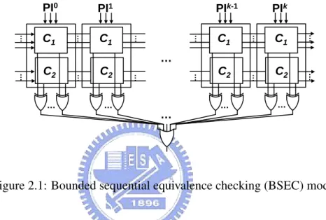
Typically, the problem of sequential equivalence checking (SEC) can be formulated as checking over time the output of the miter circuit which is composed of two finite state machines (FSMs). On the other hand, Bounded sequential equivalence checking (BSEC) [2] as shown in Figure 2.1, is a special case of SEC problems and simplifies the problem formulation by limiting the timeframes under verification to an affordable number.

PI0 _PI1 _PIk-1 _PIk C₁ C₂ C₁ C₂ C₁ C₂ C₁ C₂ … … … … … … … … … … … … … … … … … …

Figure 2.1: Bounded sequential equivalence checking (BSEC) model

Modeling a BSEC problem consists of two steps: miter construction and timeframe unfolding. The miter is constructed by linking every pair of two corresponding outputs from FSMs to one extra XOR gate. The miter is then unfolded to a user-specified number of timeframes, say k, to form the BSEC model. The combinational logic is duplicated into k copies. All flop-flops (FFs) are removed and inputs of FFs in one timeframe are connected to corresponding signals in the next timeframe. After unfolding the miter circuit, one big OR gate takes the disjunction of every output of added XOR gates from timeframe 1 to timeframe k.

Since the BSEC model is purely combinational, its satisfiability can be solved by any formal engine. If the BSEC model is unsatisfiable (UNSAT), then two circuits are proven to be equivalent under all possible input sequences over the given number of timeframes. On the other hand, if the result is satisfiable (SAT), at least one input sequence witnesses the discrepancy in k timeframes. Accordingly, two circuits can also be in-equivalent after

relaxing the bounds of timeframes to be checked.

However, the larger number of timeframe unfolding in BSEC, the better quality of ver-ification. Once the size of the BSEC model goes larger, SAT solving also becomes less efficient. Many techniques in [3] [6] have been proposed for SAT solvers to extract con-straints to early stop exploration during SAT solving. Constraint extraction is an important technique and has also been successfully applied in various electronic design automation (EDA) problems, such as logic optimization and automatic test pattern generation (ATPG). Authors in [10] [11] propose an approach of finding internal don’t-care states as constraints and merging them according to observability for Boolean network optimization. Static and dynamic learning techniques are applied in [12] [17] to guide pair-wise implications to assist test pattern generation.

Many recent studies propose different constraint extraction techniques dedicated to equivalence checking. Binary decision diagram (BDD) techniques are used to estimate the reachability of states in [23] [24] and derive the don’t care states in [19]. Equivalent state pairs can be also computed by BDD comparison to facilitate cutpoint finding [8] and to prove equivalence in a partitioning approach [9]. Association rule mining [28] and logic implication are combined in [20] [25] to derive 3-node relations among all internal nodes to facilitate SAT solving for BSEC problems.

Most of previous works [19] [20] [21] focus on the relationship of internal signals at one single timeframe. However, the primary outputs and register inputs are shown to have greater impact than internal signals in [22], and multi-timeframe constraints show to be effective for speeding up SAT solving in [20] [25]. Therefore, we are motivated to proposed a learning-and-filtering framework as shown in Figure 4.2 to uncover cross-timeframe state-pair constraints.

To avoid effort on internal signals over timeframes, our framework will learn the relaxed Boolean functions for flip-flop(FF) state at different timeframes according to a relatively small number of simulation data. FF states that can learn Boolean functions form the basis for the initial set of state-pair constraints. Furthermore, although the total number of FFs is much smaller than that of internal signals, exhaustive checking of all state-pairs is not necessary either. Multiple filtering strategies is required to reduce the total number of constraint candidates.

2.2

Boolean Satisfiability

Boolean Satisfiability (SAT) problem is a well-known constraint satisfaction problem. Given a propositional logic formula f , determining whether there exists a variable assign-ment φ that makes the formula evaluate to true. If such assignassign-ment φ exists, it indicates that f is satisfiable (SAT). Otherwise, f is unsatisfiable (UNSAT). For example, there is a satisfiable problem f = (¬y + x1)(¬y + x2)(y + ¬x1 + ¬x2), there is a solution φ(f )

satisfied the problem, which is y = 1, x1 = 1, x2. SAT is one of the central NP-complete

problems. [7]

Most solvers operate on problems for which f is specified in conjunctive normal form (CNF). This form consists of the logical AND of one or more clauses, which consist of the logical OR of one or more literals. The literal comprises the fundamental logical unit in the problem, being merely an instance of a variable or its complement denoted as ¬. The advantage of CNF is that in this form, for f to be satisfied, each individual clause must be satisfied. If any clause is unsatisfied, f is unsatisfied. Thble 2.1 lists the conjunctive normal form of some basic logic gates, where x1and x2denotes the inputs of a gate, and y denotes

the output.

Table 2.1: Conjunctive normal form of some basic logic gates

Gate type Conjunctive Normal Form

AND (¬y + x1)(¬y + x2)(y + ¬x1+ ¬x2)

OR (y + ¬x1)(y + ¬x2)(¬y + x1+ x2)

NAND (y + x1)(y + x2)(¬y + ¬x1+ ¬x2)

NOR (¬y + ¬x1)(¬y + ¬x2)(y + x1+ x2)

XOR (¬y + x1+ x2)(¬y + ¬x1+ ¬x2)(y + ¬x1+ x2)(y + x1+ ¬x2)

XNOR (y + x1+ x2)(y + ¬x1+ ¬x2)(¬y + ¬x1+ x2)(¬y + x1+ ¬x2)

NOT (¬y + ¬x1)(y + x1)

BUF (¬y + x1)(y + ¬x1)

Figure 2.2 shows a sample circuit, where I1, I2 and I3 are inputs, O is output, and G1,

The formula of the circuit is, fO = (¬G1+ I1)(¬G1+ I2)(G1+ ¬I1+ ¬I2)(G2+ I2)(G2+

I3)(¬G2+ ¬I2+ ¬I3)(G3+ ¬G1)(G3+ ¬G2)(¬G3+ G1+ G2), which is encoded by each

logic gate.

Figure 2.2: A sample circuit

The popular SAT-solvers based on the DPLL (Davis-Putnam-Logemann-Loveland) al-gorithm [13] [14], backtracking by conflict analysis and clause recording [18], and Boolean constraint propagation (BCP) using watched literals [3]. The search procedure in DPLL al-gorithm is to pick a variable heuristically and assign specific value to the selected variable, until the propagation detects a conflict. The backtracking process will continue until the conflict clause becomes unit since the assignment of the unit clause could propagate to other clauses. The search procedure stops if all variables are assigned or a conflict occurs in one variable, and the solver returns SAT and UNSAT, respectively.

Algorithm 1 is the basic procedure of DPLL-based SAT solver in MiniSAT [6]. Each run of outer loop starts from one variable assignment. If one variable has been assigned, the inner loop could use to examine the variable assignment is legal or not. The loop starts from unit clause propagation. In the conflict occurs, the algorithm will analyze the conflict and add a conflict clause to the original problem. If the conflict occurs in top-level, the solver will return UNSAT. Otherwise, if the conflict does not occur in top-level, the procedure will backtrack to undo assignments until the conflict clause is unit. If there is no conflict occurs in this loop, the algorithm will continue to decide the assignment of next variable or check if all variables are assigned.

MiniSAT [6] is a minimalistic implementation of a Chaff-like SAT solver [3]. Com-pared with Zchaff, MiniSAT provides the incremental SAT interface and support for user defined Boolean constraints. Although the performance of Zchaff and MiniSAT are similar,

MiniSAT is easy to integrate to larger system with verification techniques due to portable ability. In this work, we integrate MiniSAT to proposed verification method to solve the bounded sequential equivalence checking problem.

Algorithm 1 DPLL-based SAT solver in MiniSAT [6]

1: loop

2: propagate() //propagate unit clauses

3: if not conflict then

4: if all variables assigned then

5: return SATISFIABLE

6: else

7: decide() //pick a new variable and assign it

8: else

9: analyze() // analyze conflict and add a conflict clause

10: if top-level conflict found then

11: return UNSATISFIABLE

12: else

13: backtrack() //undo assignments until conflict clause is unit

2.3

Data Mining

Data mining technique is a technique to explore information from data. It utilizes sta-tistical method to analyze the data and exploit the most frequent pattern to represent the data. Data mining method is widely used on many fields including marketing, science and engineering. Data mining techniques incorporated with verification problem will bring about test vector selection with classification [15], process variation modeling with regres-sion [16], or constraints extraction with data correlation [20] [25].

The major procedure to apply data mining on specific problem involves the steps: prob-lem definition, training data collection, data preprocessing and model construction. For ex-ample, in this work, learning relaxed Boolean function of particular signals in miter circuit

is the objective. Training data in this case is the input pattern and response on the particu-lar signals, which could collect from amount of simulation. Data preprocessing is used to remove redundant information in training data, for example, the reset signal or clock signal in circuit. The last step is model construction, which built the simplified model for each signal through simulation.

We summarize a few examples to illustrate different types of data mining techniques on simulation data.

• Implication rule: The simplest form of mining may be the extraction of an implica-tion rule such as (X =⇒ Y ). The problem can be harder if we consider finding all these rules such that both A and B are internal signals whose total amount is large. We propose to incorporate the concept of support-confidence framework used in as-sociation rule mining and develop a similar framework to mine implication rules. • Signal correlation: We may relax the implication rule into signal correlation, denoted

as (X ∼ Y ). This means that with a probability of c, signal A and signal B change their values together. This is another type of association rule mining.

• Clustering: Given K signals, we would like to partition them into groups such that signals within the same group are highly correlated. Clustering can be an application from the result of signal correlation mining.

• Association rule: Given K signals, we would like to find a subset of signals S1 and

a subset of signals S2 such that the changes on signals in S2is most likely due to the

changes of signals in S1 (with a confidence level c). We denote this as (X ⇒ Y ).

• Statistical modeling: Given two sets of signals: S1 and S2, we would like to obtain

a statistical model f such that f (S1) can be used to predict values on S2. This is a

typical statistical learning problem. Techniques such as neural networks or compu-tational learning techniques are suitable for this problem.

2.3.1

Association Rule Mining

Association rule mining (ARM) was first introduced by Agrawal et al. in [27], which aims to extract interesting correlations, frequent patterns, association or casual structures among sets of items in the transaction database or data repository. By definition, an asso-ciation rule is an implication of the form X ⇒ Y , where X and Y are frequent itemsets in a transaction database and X ∩ Y 6= 0. Conventionally, X is called antecedent while Y is called consequent. An association rule can be further classified into four different forms, X ⇒ Y , X ⇒ ¬Y , ¬X ⇒ Y and ¬X ⇒ ¬Y . The first form is called a positive rule while all of the others are called negative rules.

When studying association rules, there are two important basic measures, (1) support and (2) confidence. Support, denoted as supp, is a statistical measure and sup(X) is defined as the fraction of records that contains the target itemset, X, to the total number of records in the database. However, confidence (denoted as conf ) of an association rule X ⇒ Y is a measure of strength and defined as the ratio supp(X ∪ Y )/sup(X) where X ∪ Y means both X and Y are present.

The support-confidence framework proposed in [27] seeks positive rules of the form X ⇒ Y with support and confidence greater than, or equal to, user-specified minimum support (γsup) and minimum confidence (γconf) thresholds, respectively, where

• X and Y are disjoint itemsets; that is, X ∩ Y 6= 0 • sup(X ⇒ Y ) = sup(X ∪ Y )

• conf (X ⇒ Y ) = sup(X ∪ Y )/sup(X)

The negation of an itemset X is indicated by ¬X. The support of ¬X, sup(¬X), is 1 − sup(X). To take a particular itemset, i1¬i2i3, for example, supp(i1¬i2i3) = supp(i1i3) −

supp(i1i2i3). Like positive rule, a negative rule (e.g. X ⇒ ¬Y ) also has a measure of its

strength, conf , defined as supp(X ∪ ¬Y )/sup(X). By extending the definition, negative association rule discovery seeks rules of the form X ⇒ ¬Y with support and confidence greater than, or equal to, user-specified minimum support (γsup) and minimum confidence

• X and Y are disjoint itemsets; that is, X ∩ Y 6= 0 • sup(X) ≥ ms, sup(Y ) ≥ ms, and sup(X ∪ Y ) < ms • sup(X ⇒ ¬Y ) = sup(X ∪ ¬Y )

• conf (X ⇒ ¬Y ) = sup(X ∪ ¬Y )/sup(X)

From the above discussion, we can conclude that association rule mining consists of two steps: finding frequent itemsets and generating rules. In general, finding frequent itemsets contains two sub-steps, candidate large itemset generation and frequent itemset generation. Minimum support (γsup) is specified from users to decide the itemsets of interest. Finding

frequent itemsets is the focus of all association rule mining algorithms. Generating rules is relatively straightforward. Possible rules of interest from the frequent itemsets are enu-merated. Then the specified minimum confidence (γconf) must be satisfied when a rule is

finally derived.

2.3.2

Support-confidence Framework

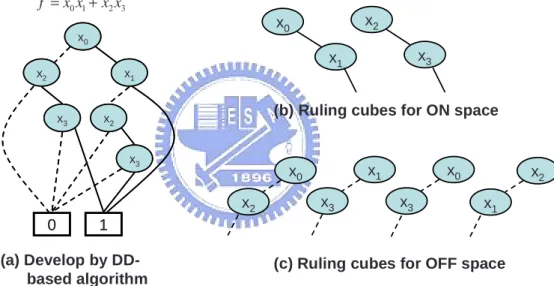
In conventional decision diagram (DD) based mining algorithm, it used simulation data to construct a decision diagram to record the functional space, as shown in Figure 2.3(a). As can be seen in the figure, it is the decision diagram of f = x0x1+ x2x3and the variable

ordering is x1 > x2 > x3. The solid line and the dotted line indicate the on space (xi = 1)

and the off space (xi = 0), respectively. The decision diagram records the row data in

the truth table of f = x0x1 + x2x3. Although the decision diagram could represent the

functional space of f , there are two weaknesses in DD-based mining algorithm. (1) good variable ordering requirement and (2) statistical information lack for variable splitting. Al-though DD-based mining algorithm can handle verification problem such as reachability analysis, the variable ordering problem is still a bottleneck for such algorithm to drive the circuit with deeply sequence. During model generation by such mining algorithm, the learning model may be biased by noise information due to lack the statistical information for variable splitting. The two weaknesses of DD-based mining approach will limit its ability to apply on high complexity circuit.

To avoid weaknesses of DD-based algorithm, a new mining algorithm considering sta-tistical information will be developed. This new approach is based on DD-based mining method and support-confidence method in section 2.3.1. It considers the statistical infor-mation while variable splitting and generate rule-based model instead of diagram-based model. The goal of this approach is to extract abstraction view of circuit through simu-lation, and the ruling results can be taken as bigger Boolean cubes in functional space of circuit. The ruling results are so called ruling cubes shown in Figure 2.3(b) and 2.3(c). In Figure 2.3(b), the ruling cubes x0x1 and x2x3 represents the ON space. That is mean both

x0x1 and x2x3 will imply f = 1 . For the same concept, Figure 2.3(c) shows the ruling

cubes for OFF space.

x₀ x₂ x₁ x₃ x₂ x3 0 1 x₀ x₂ x₁ x₃ x₂ x3 0 1 x₀ x₁ x₂ x₃ 0 1 2 3 f =x x +x x x₀ x₂ x₁ x₃ x₀ x₃ x₂ x₁ (a) Develop by DD-based algorithm

(b) Ruling cubes for ON space

(c) Ruling cubes for OFF space

Figure 2.3: Example of ruling cubes

The ruling cubes are generated by taking the statistical information into account. First of all, a supporting variable method will explore the best spilting variable in each process. Next, the support-confidence measurement introduced in section 2.3.1 will calculate the sup and conf rate to quantify the ruling cube. If the sup and conf of ruling cube reach the minimal support (γsup) and minimal confidence (γconf) threshold, the ruling cube will

be extracted. At the same time, the training data explained by the extracted ruling cube will be removed and the remaining data will continue to extract other ruling cubes. On the

other hand, if the sup and conf of ruling cube do not reach the γsupand γconf threshold,

the supporting variable method will be applied to select another spilting variable until the ruling cube satisfying the ms and mc requirement. The detail algorithm will be introduced in section 3.2.

Return to the bounded sequential equivalence checking problem. The mined ruling cubes can be constructed the approximate function for each state (output of flip-flop) at some timeframe, the unreachable cross-timeframe can be examined by checking the inter-section of functions for two arbitrary states. If the interinter-section is empty, then this state pair can be considered as a candidate of unreachable state pair. These unreachable state pairs will be set as constraints and apply to facilitate BSEC problem.

Chapter 3

3.1

Training Data Collection

random test

generation input testinput testpatternspatterns

logic

simulation simulationsimulation_datadata

data partitioning 1-timeframe database 1-timeframe database 2-timeframe database 2-timeframe database k-timeframe database k-timeframe database …

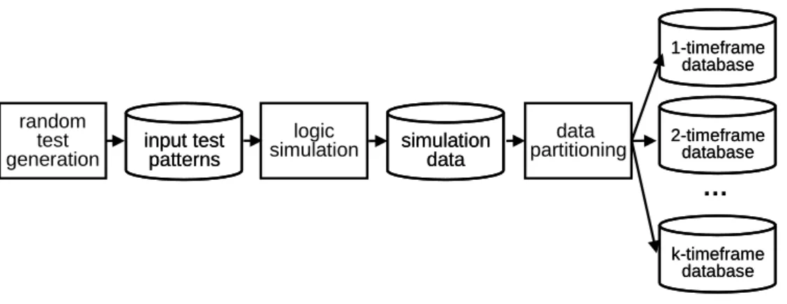
Figure 3.1: Flow of random simulation

The flow of random simulation is illustrated in Figure 3.1. First, a small number of test patterns are randomly generated and run through a logic simulator to collect the data from I/O and FFs. Then data partitioning prepares k (empirically, k = 10) databases of different timeframes for later learning. For example, for a finite state machine M with 4 PIs, 1 PO and 3 FFs, table 3.1(a) shows the simulation data after logic simulation. Since the FFs can be divided into PPOs and PPIs, each PPO value at one timeframe will be PPI value at the next timeframe. Given k = 2, 1-timeframe database collects PI and PPI data as input values and PO data as its output value from each single timeframe. 2-timeframe database collects PI and PPI data from every two consecutive timeframes but only collects PPO as its output only from the latter timeframe. Table 3.1(b) and Table 3.1(c) show the 1-timeframe database and 2-timeframe database, respectively.

3.2

Learning Relaxed Boolean Function

3.2.1

Support-confidence Method

The original concept the support-confidence framework [27], is the measurement of fre-quency pattern by counting the simulation data. Applying the support-confidence frame-work to Boolean data learning, the support sup and the confidence conf denote the fre-quency and the accuracy for one Boolean cube, respectively, on the basis of the database M . The formal definitions of support and confidence are given as follows.

Table 3.1: Partitioning data into databases

(a) raw data

time PI PPI PO PPO

0 1010 XXX 1 000 1 1111 000 0 101 2 0011 101 0 110 3 1101 110 1 011 4 1011 011 0 001 ... ... ... ... ... (b) 1-timeframe db. (c) 2-timeframe db.

input output input output

1010XXX 1 1010XXX1111000 0 1111000 0 11110000011101 0 0011101 0 00111011101110 1 1101110 1 11011101011011 0 1011011 0 ... ... ... ... ... ... sup ≡ |X| |M | & conf ≡ |X ∩ Y | |X|

where M denotes the set of total tests in the database, X denotes the set of tests covered by one Boolean cube, Y denotes the set of tests with the target output response (either 0 or 1) in M , and |.| denotes the size of one set.

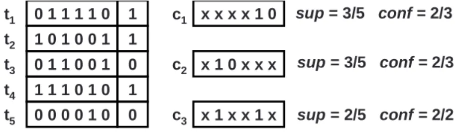
Each Boolean function of one FF state can be approximated by a set of Boolean cubes. For example, in Figure 3.2, {ti} denotes the test set in simulation database M and {ci}

denotes the set of Boolean cubes to be evaluated. For each cube ci, two corresponding

metrics, support and confidence (denoted as supi and confi), are used to quantify the

im-portance of such a cube. If both supi and confi are larger than the threshold values, γsup

and γconf, respectively, then the cube ci is a ruling cube and can be used to construct the

relaxed Boolean function F∗ later. In contrast, those Boolean cubes that fail to satisfy the support and confidence criteria will be excluded in F∗.

0 1 1 1 1 0 1 1 0 1 0 0 1 1 0 1 1 0 0 1 0 1 1 1 0 1 0 1 0 0 0 0 1 0 0 x x x x 1 0 x 1 0 x x x x 1 x x 1 x sup = 3/5 conf = 2/3 sup = 3/5 conf = 2/3 sup = 2/5 conf = 2/2 t₁ t₂ t₃ t₄ t₅ c₁ c₂ c₃

Figure 3.2: Example of support-confidence learning

Figure 3.2 shows an example of support-confidence learning. Given the database M = {t1, ..., t5}, the cube c1 satisfies t1, t4 and t5 and sup1 is 3₅. However, since only t1 and t4

have the target output response (y = 1), conf1 is 2₃. supiand confiof any other cube i can

be computed in the same manner. Moreover, suppose that γsupand γconf are 0.05 and 0.95,

only c3 satisfies the support and confidence criteria among three cubes and also is the only

ruling cube on the basis of M in this example.

Support-confidence learning algorithm is proposed to derive the set of ruling cubes for constructing the relaxed Boolean function for each flip-flip state. In Figure 3.2, c3= x1xx1x

represents one ruling cube x2x5 where x2 and x5 are support literals which represent the

most important variable states in such a ruling cube. One ruling cube is generated by adding the support literal one by one until no further support literal can be found.

3.2.2

Impurity Measure

According to [26], the impact of one variable state can be achieved by comparing the impurity difference between the original database M and the new Mv split with respect

to one variable state v. In short, the support variable with maximum gain is the most important variable of the given database. For two literals (x and x) of one input variable and the database M , g(x) and g(x) can be formulated as

g(x) ≡ n11 n10+ n11+ 1

& g(¯x) ≡ n01 n00+ n01+ 1

where n11is the number of tests with input variable x = 1 and output response y = 1, n10

is the number of tests with x = 1 and y = 0, n01 is the number of tests with x = 0 and

Note that g(x) represents the ratio of the number of tests with x = 1 and y = 1 to the number of all tests with x = 1 in M ; g(x) can be understood similarly. After the gain values of all variable states are computed, the variable state with maximum gain will be selected as the next support literal.

0 1 1 1 1 1 1 0 0 1 0 1 1 1 0 0 0 0 1 1 0 0 1 0 0 0 0 1 0 0 0 0 f x₁x₂x₃ 0 1 1 1 1 1 1 0 0 1 0 1 1 1 0 0 0 0 1 1 0 0 1 0 0 0 0 1 0 0 0 0 f x₁x₂x₃ 2/5 1/5 2/5 0 1/5 0 2/5 1/5 2/5 2 1 2 n11 2 3 2 n10 0 1 0 n₀₁ 4 3 4 n00 x₃ x₂ x₁ 2/5 1/5 2/5 0 1/5 0 2/5 1/5 2/5 2 1 2 n11 2 3 2 n10 0 1 0 n₀₁ 4 3 4 n00 x₃ x₂ x₁ ( ) g x ( ) g x ( ) gain x 1 v=x c=x1 1 1 . 2 2 c sup= c.conf = 0 1 1 1 1 0 0 0 1 1 0 0 f x₂x₃ 0 1 1 1 1 0 0 0 1 1 0 0 f x₂x₃ 2/3 1/3 2/3 1/3 0 1/3 0 1 n₁₁ 2 1 n₁₀ 2 1 n₀₁ 0 1 n₀₀ x₃ x2 2/3 1/3 2/3 1/3 0 1/3 0 1 n₁₁ 2 1 n₁₀ 2 1 n₀₁ 0 1 n₀₀ x₃ x2 ( ) g x ( ) g x ( ) gain x 3 v=x c=x x1 3 1 . . 1 4 c sup= c conf =

(a) select the first support variable (b) select the next support variable

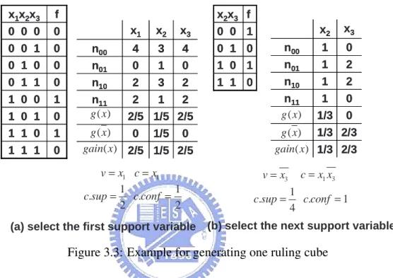
Figure 3.3: Example for generating one ruling cube

Figure 3.3(a) illustrates the process for selecting the first support literal. The original database M has three inputs, x1, x2, and x3. The values of {n00, n01, n10, n11} for each

variable state is first computed. For example, {n00, n01, n10, n11} for x1is {4, 0, 2, 2}, and

thus, g(x1) = ₂₊₂₊₁2 and g(x1) = ₄₊₀₊₁0 . g(x2), g(x2), g(x3) and g(x3) can be computed

similarly. After all gain values are available, the variable state with the maximum gain is selected as the support literal. If two variable states have the maximum gain, the support literal can be selected arbitrarily. In our example, both x1 and x3 have the maximum gain

2

5, and x1 is chosen arbitrarily to be the first support literal for the ruling cube c.

Given γsup= 0.05 and γconf = 0.95, for the current rule cube c = x1, supc=

|M_x1=1| |M | is 4 8and confc= |M_x1=1∩y1=1| |M_x1=1| is 2

4. Since the current confcis much lower than γconf, the ruling

cube generation will continue to find the next support literal as shown in Figure 3.3(b). Note that the database M now becomes Mx1=1since the next support literal needs to be selected on the basis of all tests with x1 = 1 in M .

Once the extracted Boolean cube c meets supc ≥ γsup and confc ≥ γconf, it will be

accumulated in the set of ruling cubes for constructing the approximate function of one flip-flop state later. However, if no other variable state can be selected and the current cube fails to meet the support and confidence criteria, the cube will be dropped. To avoid processing the same cubes, both the tests covered by ruling cubes and dropped cubes will be removed from the database.

Algorithm 2 shows the overall algorithm to construct the approximate function for one flip-flop state. Given database M , N is the maximum number of support literals in one ruling cube since the maximum number of literal to split database M is log2|M |. F∗ is the

target function to be extracted and D is the set of current tests covered by F∗.

The algorithm starts from constructing a Boolean cube representing a sub-function f by adding one variable state one at a time. SupV arSelect() is applied to select the next support literal x under f . When both the frequency fsupand the accuracy fconf can meet

the criteria, f is updated by conjuncting itself with x. The algorithm keeps finding the next support literal to update f until the current cube f has met the ruling cube criteria in line 9 or included more than N variable states in line 13. F∗continues accumulating ruling cube f0s for one flip-flop state until F∗covers a percentage γcovof the total tests in the database

M .

Note that according to the learning theory, the quality of a data-mining algorithm de-pends upon the data complexity, not the structural complexity underlying. Therefore, given a small number of simulation data, the FF state at the smaller k-th timeframe seems rela-tively easy to learn its relaxed Boolean function. However, for those FF state at the large k-th timeframe, more simulation may be needed but not necessary. Since learning for re-laxed Boolean functions is one-time cost, the user can allocate a sufficient amount of time for his BSEC problems.

Algorithm 2 SupportConfidenceLearning(): a support-confidence learning algorithm with the impurity measure

1: N = log2|M |; 2: F∗ ← ∅; 3: while (D≤  M× γcov) 4: f = 1; 5: do {

6: x = SupVarSelect(M, f ); // impurity measure 7: f ← f ∩ x;

8: update(fsup,fconf); // update fsupand fconf 9: if (fsup≥ γsup&& fconf ≥ γconf)

10: F∗ ← F∗ _{∪ f ;}

11: update(D); // update by ruling cube

12: break;

13: } while (|f | < N );

14: if (fsup< γsup&& fconf < γconf)

Chapter 4

4.1

Constraints in BSEC Problem

Figure 4.1 is an example to illustrate how the conflict constraints work on the SAT solving process, Before the example, let’s recall the basic idea in SAT solving. The DPLL-based algorithm, introduced in section 2.2, is the core of most start-of-art SAT engines. The procedure of DPLL-based algorithm is illustrated as follows:

1. Trace from the clause with minimum number of literals, especially in unit clause Assign value to variable v, and push v into assignment queue

2. Use v to apply implication on other clauses

If variable u could be implied by v, then push u into assignment queue

3. While size of assignment queue is equal to the number of variables, return SAT if implication v0 6= v in assignment queue, return UNSAT

In DPLL-based algorithm, the assignment queue is used to record the assigned vari-ables. Since all clauses in a SAT problem must be satisfable and the problem can be satis-fiable. DPLL-based algorithm starts from the clause with minimum number of literals. If one variable v could be assigned the specific value, the variable could be pushed into the as-signment and propagated to other clauses. The procedure would continue to assigned other variables. If all variables have been assigned, the problem is satisfiable. If one implied variable conflicts the results in assignment queue, the problem is unsatisfiable.

V₁ V₂ V₃ V₄ V₅ V₆ V₇ V1 V2 V5 V6 0 0 0 1 1 0 1 1 0 0 0 1 1 0 0 0

(a) a simple circuit (b) truth table of V₅and V₆

V₁ V₂ V₃ V₄ V₅ V₆ V₇ V1 V2 V5 V6 0 0 0 1 1 0 1 1 0 0 0 1 1 0 0 0 V₁ V₂ V₅ V₆ 0 0 0 1 1 0 1 1 0 0 0 1 1 0 0 0

(a) a simple circuit (b) truth table of V₅and V₆

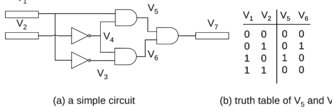
Figure 4.1(a) is the sample example and Figure 4.1(b) is the truth table of V5and V6 in

sample circuit. From the truth table, it implies that the logic value of V7is stuck at 0. If the

circuit is modeled as a SAT problem and target V7 = 1, the SAT engine is expected to return

an unsatisfiable answer. Table 4.1 lists the clauses of the sample circuit in Figure 4.1(a). Table 4.1: Clauses for Figure 4.1

1 ¬V5+ V1 8 V4+ V2 2 ¬V5+ V4 9 ¬V3+ ¬V1 3 V5+ ¬V1+ ¬V4 10 V3+ V1 4 ¬V6+ V2 11 ¬V7+ V5 5 ¬V₆+ V3 12 ¬V7+ V6 6 V6+ V2+ V3 13 V7+ ¬V5+ ¬V6 7 ¬V₄+ ¬V2 14 V7

The procedure is used to solve the SAT problem, as follows:

• step1: start from unit clause 14, imply V7 = 1, push V7into assignment queue

• step2: process V7, imply V5 = 1 in clause 11 and imply V6 = 1 in clause 12,

push V5 and V6into assignment queue

• step3: process V5, imply V1 = 1 in clause 1 and imply V4 = 1 in clause 2,

push V1 and V4into assignment queue

• step4: process V6, imply V2 = 1 in clause 4 and imply V3 = 1 in clause 5,

push V2 and V3into assignment queue

• step5: process V1, imply V3 = 0 ←→ conflict with V3 = 1,

return UNSAT.

In the procedure, it requires five steps to prove the SAT problem in Table 4.1 is unsat-isfiable. Although the five steps seems not heavy, it would be difficult as solving larger circuits. Conflict constraints are one way to speedup the proof. From the truth table in

Figure 4.1, it is clearly to observe that the V5 = 1 and V6 = 1 can not happen at the same

time. we call that (V5, V6) is a conflict constraint in the sample circuit and add the conflict

constraint as a conflict clause after original SAT problem. Since (V5, V6) means V5 = 1

and V6 = 1 can not happen at the same time, it indicates V5 = 0 and V6 = 0 may occur

in the circuit. As a result, the clause of (V5, V6) can be written as ¬V5+ ¬V6 and added as

15th clause after original SAT problem. The solving procedure of new SAT problem is as follows,

• step1: start from unit clause 14, imply V7 = 1, push V7into assignment queue

• step2: process V7, imply V5 = 1 in clause 11 and imply V6 = 1 in clause 12,

push V5 and V6into assignment queue

• step3: process V5, imply V1 = 1 in clause 1 and imply V4 = 1 in clause 2,

imply V6 = 0 in clause 15 ←→ conflict with V6 = 1, return UNSAT.

Compare with solving the original SAT problem, the SAT problem with a conflict straint only requires 3 steps of proof. The example illustrates the power of conflict con-straints. Since the BSEC problem is a combinational SAT problem and the solving process is similar to the BCP procedure, and the conflict constraints will also help SAT solving.

One way to find out conflict constraints in BSEC is to list the truth table for all internal signals and discover the unhappen situation in the truth table. However, it is impossible to enumerate all input combination to construct such truth table as in Figure 4.1(b). The alternative method is to construct the relaxed Boolean function of each signal, as mention in section 3.2. Since the number of combination of internal signals is quite large, in this work, we only extract the information on flip-flops. The detail explanation is introduced in section 2.1.

The previous work in [20] is the first study of applying a support-confidence algorithm named Apriori to explore the implication constraints among 3 internal nodes (a·b→c) for SAT solving. However, in this work, we do not mine constraints directly from data. Instead, we propose a new learning algorithm which modifies the notion of support-confidence with impurity measures [28] to infer the relaxed Boolean functions for each FF state at different timeframes. Later, conflict constraints will be derived by composing two relaxed Boolean

functions.

DEFINITION (Conflict Constraint)

A state-pair (pi,qj), where i, j denote the timeframes and j > i > 0, in a finite state ma-chine M is a conflict constraint if and only if ∀k > i, qk+j−i can never appear after pk appears in M for all input sequences.

Such constraints can be used to early stop the random walk during the SAT solving process, and their effectiveness will be demonstrated through our experiments later. The proposed method to exploit conflict constraint is introduced in the following section.

4.2

3-stage Filtering Method

Since previous studies [19] [20] that explore the constraints among internal nodes for SAT solving may suffer from a large number of constraint candidates, the proposed method instead considers cross-timeframe state-pairs as candidates and prunes the false cases on the basis of simulation data and the gate-level netlist of the circuit.

Since each state-pair can be validated by running SAT solving on the BSEC model, one intuitive method is to enumerate all combinations of state-pairs for checking. How-ever, given n and k are the numbers of flip-flops and the number of timeframe unrolling, respectively, the combinations for state-pairs will go up to 4 × C₂nk, where 4 represents dif-ferent cases of state-pairs including {00}, {01}, {10}, and {11}. Running SAT solving for 4 × C₂nktimes will be prohibitively time-consuming and even worse than solving the BSEC model directly. Therefore, a 3-stage constraint extraction shown in Figure 4.2 integrates multiple filtering strategies to help reduce the total number of state-pairs.

The first stage is functional filtering. A data-mining algorithm called the support-confidence framework is developed to construct the approximate Boolean functions for each flip-flop state at one specific timeframe by learning the simulation data. Then, the cross-timeframe state-pair could be a constraint candidate if the conjunction of Boolean functions for two such flip-flop states is empty. Historical filtering in the second stage scans

through the simulation data to prune the rare cases escaped from approximate functional learned in the first stage. The final stage is structural filtering which validates the candidate through SAT solving of the augmented miter circuit. Note that functional filtering plays an important role in the proposed method and needs generating as few candidates as possible to make the historical filtering and structural filtering efficient in time.

The details of the proposed method, including 3-stage constraint extraction, will be elaborated as follows. random simulation support-confidence learning constraint candidates constraint candidates functional filtering historical filtering structural filtering learning functionslearning functions simulation data simulation data constraint insertion & SAT solving

le a rn in g p h a s e fi lt e ri n g p h a s e s o lv in g p h a s e

Figure 4.2: A learning-and-filtering framework for BSEC

4.2.1

Functional Filtering

As defined in the previous section 4.1, conflict constraints can be obtained by taking the conjunction of the relaxed Boolean functions for two states at different timeframes.

SAT solver will be then applied to the conjunctive function. For example, given f (si_p) and f (sj_q) as the functions for the state si

p of FF p at timeframe i and state sjq of FF q at

timeframe j, respectively, If f = f (si

p) ∩ f (sjq) is UNSAT, there exists no input test which

can satisfy both FF states at individual timeframes concurrently. Therefore, (f (si_p), f (sj_q)) is one constraint candidate. Note that, for each FF r at timeframe k, the support-confidence learning algorithm will run twice: one for ON state sk

r, and the other for OFF state skr.

4.2.2

Historical Filtering

After generating the initial set of cross-timeframe state-pairs for constraint candidates, historical filtering prunes those pairs that have already been seen in simulation data. For example, given (sk_p, sk+2

q ) as the constraint candidate to be checked, if FF p in some

time-frame k has the state value of 0 and FF q in two timetime-frames later has the state value of 1, then (sk_p, sk+2_q ) will be removed from the candidate set. This situation happens because the support-confidence learning is statistical and may overlook small Boolean cubes resulted from some patterns.

4.2.3

Structural Filtering

m p

s

n q

s

Figure 4.3: Illustration for structural filtering

At this stage, structural filtering is to ensure the validity of each candidate under the unfolded miter. The logic cones of individual FF states will be extracted first and combined by an extra AND gate. Such an augmented circuit is termed augmented constraint circuit (ACC). SAT solving is performed on the ACC by enforcing the output of the AND gate

as one. If the ACC is UNSAT, such a state-pair is a true conflict constraint. Otherwise, it should be removed from the candidate set. To give an example, if (sm_p , sn

q) is one constraint

candidate, the inverted output of flip-flop p at timeframe m and the output of flip-flop q at timeframe n are connected by an extra AND gate. Such an example is illustrated in Figure 4.3. Next, SAT solving is performed on the corresponding ACC with enforcing 1 on the output of the extra AND gate. If the result is UNSAT, (sm

p , snq) is a true constraint;

otherwise, (sm_p , sn

q) should be removed.

4.2.4

Constraint insertion

Constraint insertion is the final step in the proposed framework. Given k as the number of timeframe unfolding in BSEC problems, each extracted constraint will be translated into multiple CNF constraint clauses of disjunction of inverting two FF states over k timeframes and appended to the CNF of the original BSEC model. For example, if (s2₁, s3₅) is one proven constraint, CNF clauses (s2₁+ s3₅), (s3₁+ s4₅),..., (sk−1₁ + sk₅) will be appended to the original CNF for final SAT solving.

Chapter 5

The proposed method is implemented in C++. The experiments are run on Linux equipped with a 2.4GHz CPU and 2GB RAM. ISCAS 89 and ITC 99 circuits are used as benchmarks for bounded sequential equivalence checking. Each circuit is synthesized with 10 different configurations by Design Complier from Synopsys. MiniSAT 2.0 [3] is the one of state-of-the-art SAT solvers and applied for SAT solving in our experiments. The default number of tests for simulation ranges from 1, 000 to 5, 000 depending on the number of primary inputs of the benchmark circuits. γsupand γconf are by default 0.05 and

0.95, respectively. The number of upper bound for constraint state-pairs to be inserted in functional filtering is 2, 000.

Table 5.1: Characteristics of BSEC models for benchmark circuits

miter # of PI # of PO # of FF # of k # of FF × in miter timeframes k-timeframes

s298 3 6 28 40 1120 s349 9 11 30 40 1200 s713 35 23 36 30 1080 s832 18 19 10 30 300 s1196 14 14 36 30 1080 s1488 8 19 12 30 360 s4863 49 16 169 15 3035 s15850 77 150 1040 15 15600 s35932 35 320 3456 10 34560 s38584 38 304 2690 10 26900 b04 8 11 132 30 3960 b11 7 6 60 30 180 b13 10 10 102 30 3060 b15 36 70 834 15 12510

Table 5.1 shows the characteristics of BSEC models for ISCAS 89 and ITC 99 circuits in our experiments. # of PI and # of PO are the numbers of primary inputs and primary outputs for each circuit, respectively. # of FF is the number of the flip-flops in the original miter. k is # of timeframes to be unrolled in the BSEC model. # of FF × k-timeframe

denotes the total numbers of the flip-flops in the BSEC model.

Table 5.2 demonstrates the effectiveness of 3-stage filtering by reporting the numbers of constraint candidates across different timeframes after each filtering. Column 1 lists the name of the benchmark circuits while column 2 represents the initial number of constraint candidates. Column 3, 4 and 5 denote the numbers of candidates after functional, historical and structural filterings, respectively.

Table 5.2: Comparison of numbers of constraint candidates

miter # of cross-timeframe constraints

initial functional historical structural filtering filtering filtering

s298 6160 59.3 44.9 27.3 s349 7080 217.8 110.0 109.9 s713 10224 6.2 5.1 5.1 s832 760 88.3 63.3 30 s1196 10224 78.7 57.3 42.9 s1488 1104 88.0 52.9 52.8 s4863 227812 2000 312.9 310.2 s15850 8648640 4000 2631.3 2381.7 s35932 95537664 2000 1336.0 1105.0 s38584 57878040 2000 1214.4 825.6 b04 138864 2000 1783.2 1298.1 b11 28560 2000 1643.9 1138.2 b13 82824 2000 1122.2 939.0 b15 5561112 2000 1238.1 1732.8

Table 5.3 shows the improvement of SAT solving for BSEC problems. Column 1 lists the name of the benchmark circuits and column 2 is the # of unfolded timeframes. Column 3 represents the combined runtime for both learning and filtering. Column 4 and 5 denote the runtime of SAT solving without and with constraints, respectively. Column 6 reports the speedups computed by the original runtime in Column 4 divided by the new runtime in

Column 5.

Table 5.3: Runtime for BSEC problems

miter ktime- learning original (s) new (s) speedup (X) frames time (s) [A] [B] [A]/[B]

s298 40 1.0 13.3 0.2 66.5 s349 40 1.5 3.8 0.2 19.0 s713 30 7.7 6328.3 176.2 35.9 s832 30 3.9 8.8 0.4 22.0 s1196 30 8.6 14.4 13.3 1.1 s1488 30 3.9 13.0 2.7 4.8 s4863 15 180.4 7319.9 26.9 272.1 s15850 15 2684.3 7823.1 23.7 330.1 s35932 10 1135.3 7503.9 14.3 524.7 s38584 10 529.9 2077.5 11.8 176.1 b04 30 28.6 3485.2 0.5 6070.4 b11 30 41.2 35.9 0.9 39.9 b13 30 15.6 8.0 0.2 40.0 b15 15 335.1 4897.8 8.1 604.7

Our experimental results show different speedups on SAT solving of benchmark BSEC circuits with an average as 500X, excluding the time for learning and filtering. Significant improvement can be observed on the big circuits while minor improvement can be observed on the small circuits. We also shows the speedups on 4 large circuits, s35932, s38584, b13 and b15 with respect to 10 configurations in Figure 5.1. Although for each case, 10 configurations result in different speedups but the all speedups are of the same order.

We compare the results with [20], which used association rule to imply three nodes relation on internal signals. Column 1 lists the name of the benchamrk circuits, which is the same as in [20]. Column 2 is the # of unrolled timeframes. Column 3, 4 and 5 denote the runtime of SAT solving without constraint, runtime for SAT solving with constraints, the combined runtime of mining time and SAT solving time, respectively. Column 6 reports the

speedups computed by Column 3/Column 5. Column 7 is the result excerpted from [20]. The results are only from one configuration in circuits.

miter k time origin(s) new(s) mining our speedup

frames +new(s) speedup [20]

s298 40 30.39 0.12 9.25 3.29 3.11 s832 30 2028.65 0.72 6.41 316.48 50.30 s1196 30 96.19 55.78 79.98 1.20 2.59 s1488 30 754.03 5.68 21.70 34.75 33.93 s4863 15 7725.44 4.35 236.02 32.73 15.07 s15850 15 64860 227.63 1593.46 40.71 40.28 s35932 10 51744.3 173.78 1397.12 37.04 4.54 s38584 10 50464.3 19.50 1221.10 41.33 3.43

Table 5.4: Runtime for BSEC problems compare with [20]

Since we do not know the configuration of circuit used in [20], the comparison may be not faired. However, the results should be focused on the speedup in our approach and their result. Compared with results from [20], not all of cases with our approach would have such benefit because the effective of conflict constraints is depended on the property of circuit. Our approach only finds out constraints between states with different timeframes, but in [20], they consider about internal nodes. Different circuits may agree with different approaches. However, the results show that our approach is overall good in most cases. By the way, in [20], they explained that their approach has less improvement in easy miters, so they only reported hard miters. The same problem we meet. It is because the complexity is depended on the number of flip-flops, and the computation time of exploring constraints in easy miter is almost the same as in hard miters. So there is no obviously improvement in easy miter with our approach.

To demonstrate the effectiveness of the extracted constraints, we compare the numbers of timeframe unfolding on 4 large benchmark circuits without and with the extracted con-straints in a fixed time, say 1200 seconds in our experiments. In Figure 5.2, the dotted lines denote the original benchmark circuits while the solid lines represent the benchmark circuits with extracted constraints. Results show that after adding constraints, the bound

k can increase from 8X to 20X. It also means that the quality of BSEC can be improved greatly by applying our framework. However, different time limits may result in different improvements.

We further investigate the relations between the number of constraints and runtime for SAT solving on three big ISCAS 89 circuits. Figure 5.3 shows the result where Y-axis represents the runtime for new SAT solving normalized to the original runtime used by SAT solving without any constraint. Obviously, s35932 and s38584 converge fast and only require 500 constraints while s15850 may require 1900 constraints to converge. However, since not each constraint has same contribution to SAT solving, the efficiency of solving BSEC may depend on the quality of constraints, not the number of constraints. Therefore, how to select enough good constraints to fast converge SAT solving is worth investigation and can be a topic for future research.

0 1 0 0 2 0 0 3 0 0 4 0 0 5 0 0 1 2 3 4 5 6 7 8 9 1 0

c

o

n

fi

g

u

ra

ti

o

n

i

n

d

e

x

sp

ee

du

p (

X)

0 5 0 1 0 0 1 5 0 2 0 0 2 5 0 3 0 0 1 2 3 4 5 6 7 8 9 1 0

c

o

n

fi

g

u

ra

ti

o

n

i

n

d

e

x

sp

ee

du

p (

X)

0 2 0 4 0 6 0 8 0 1 0 0 1 2 3 4 5 6 7 8 9 1 0

c

o

n

fi

g

u

ra

ti

o

n

i

n

d

e

x

sp

ee

du

p (

X)

0 2 0 0 4 0 0 6 0 0 8 0 0 1 2 3 4 5 6 7 8 9 1 0

c

o

n

fi

g

u

ra

ti

o

n

i

n

d

e

x

sp

ee

du

p (

X)

(a

)

s

3

5

9

3

2

(b

)

s

3

8

5

8

4

(c

)

b

1

3

(d

)

b

1

5

0 1 5 3 0 4 5 6 0 7 5 9 0 1 2 3 4 5 6 7 8 9 1 0

c

o

n

fi

g

u

ra

ti

o

n

i

n

d

e

x

# o

f t

im

efr

am

e

n ew o ri g in al 0 5 0 1 0 0 1 5 0 2 0 0 2 5 0 1 2 3 4 5 6 7 8 9 1 0

c

o

n

fi

g

u

ra

ti

o

n

i

n

d

e

x

# o

f t

im

efr

am

e

n e w o ri g in a l 0 4 0 8 0 1 2 0 1 6 0 2 0 0 1 2 3 4 5 6 7 8 9 1 0 c o n fi g u ra ti o n i n d e x

# o

f t

im

efr

am

e

n e w o ri g in a l 0 2 0 4 0 6 0 8 0 1 0 0 1 2 0 1 4 0 1 2 3 4 5 6 7 8 9 1 0 c o n fi g u ra ti o n i n d e x # o f t im efr am e n e w o ri g in a l

(a

)

s

3

5

9

3

2

(b

)

s

3

8

5

8

4

(c

)

b

1

3

(d

)

b

1

5

Figure 5.2: Bound for SAT solving of BSEC problems with and without constraints

0 0.2 0.4 0.6 0.8 1 0 600 1200 1800 2400 3000 # of constraints N o rm a li z e d t im e ( s ) s15850 s35932 s38584

Chapter 6

Conclusion

The general problem of checking functional equivalence for two sequential circuit is still far from being solved. In this thesis, we proposed a method which integrates data mining, simulation and structural analysis techniques to extract unreachable cross-timeframe state-pairs as constraints to facilitate SAT solving for bounded sequential equiv-alence checking (BSEC) problems.

To exploit conflict constraints in BSEC problem, we propose a 3-stage filtering method. They are functional filtering, historical filtering and structural filtering. In functional filter-ing, we propose a new data mining method to construct relaxed Boolean function for partic-ular signals. Instead of using decision diagram to construct Boolean function, our support-confidence method with impurity measure provides statistical perspective on Boolean func-tions. In historical filtering, we use simulation information to prune the false candidate in functional filtering since the goal of the learning model is simple instead of precise. The fi-nal stage is structural filtering. Since the remain constraints behind first two stages are from limited simulation data, the result may be not global true in BSEC model. To make sure the extracted constraints are global true, each of they should be injected into the original SAT problem to be verified.

Experimental results shows that the 3-stage filtering can derive the set of unreach-able cross-timeframe state-pairs efficiently. SAT solving with the extracted constraints can speed up 3X to 300X on most ISCAS 89 and larger ITC 99 circuits. We also demonstrate that the rate of timeframe expansion could be grown on 8X to 20X.

Future works include the quality analysis of the extracted constraints and a better strat-egy to exploit constraints efficiently. Moreover, instead of conflict constraints, we will exploit other kinds of constraint. Since some circuits may be hard to exploit conflict straints, such BSEC problems are difficult to improve. In the future, the procedure of con-straint extraction can be integrated into sequential SAT solver to improve the performance the sequential equivalence checking problem.