應用於時變與非時變OFDM系統之新通道估測法

國 立 交 通 大 學

電信工程學系碩士班

碩士論文

應用於時變與非時變

OFDM 系統之

新通道估測法

New Channel Estimation Methods for Time

Invariant/Variant OFDM Systems

研 究 生：楊植纓

指導教授：吳 文 榕 博士

應用於時變與非時變

OFDM 系統之新通道估測法

New Channel Estimation Methods for Time Invariant/Variant

OFDM Systems

研 究 生：楊植纓 Student：Chih-Ying Young

指導教授：吳文榕 博士 Advisor：Dr. Wen-Rong Wu

國 立 交 通 大 學

電信工程學系碩士班

碩 士 論 文

A Thesis

Submitted to Department of Communication Engineering

College of Electrical and Computer Engineering

National Chiao-Tung University

in Partial Fulfillment of the Requirements

for the Degree of

Master of Science

In

Communication Engineering

July 2009

Hsinchu, Taiwan, Republic of China

應用於時變與非時變

OFDM 系統之新通道估測法

New Channel Estimation Methods for Time Invariant/Variant

OFDM Systems

研究生：楊植纓 指導教授：吳文榕 教授

國立交通大學電信工程學系碩士班

摘要

通道估測(channel estimation)通常是依靠系統中的領航訊號(pilot)來完成。當通道 的時間延遲較長時，估測效能可能會因為受限於有限的領航訊號而下降。最近有研究 者在 DVB-T 系統下提出的聯合時域和頻域通道估測法，比舊有頻域通道估測法的效能 好很多。然而，因為這個估測方法需要四個 OFDM 訊號的資訊來完成，所以對於記憶體 的使用量大，在時變通道中也不適用。在本篇論文中，我們提出了一個新的通道估測 法來解決此問題。在本篇論文的第一部分，我們提出適用於非時變通道的新通道估測 法，而在本篇論文的第二部分，我們延伸此新通道估測法，使它適用於時變通道的估 測。我們所提出的通道估測法，最主要的特色是即使在領航訊號(pilot)密度很低時， 也只需要一個 OFDM 訊號就可以完成。而從模擬結果也可以看出，我們所提出的通道估 測法有很好的效能。

New Channel Estimation Methods for Time Invariant/Variant

OFDM Systems

Student: Chih-Ying Young Advisor: Dr. Wen-Rong Wu

Department of Communication Engineering

National Chiao-Tung University

Abstract

In pilots-aided OFDM systems, the channel estimation relies on the pilots inserted in the systems. Since the number of pilots is usually limited, the performance of the channel estimate may not be satisfactory when the delay spreard of the channel is large. Recently, a joint time and frequency domain estimator, which can grealty outperform the conventional frequency domain channel estimator, has been proposed for DVB-T systems. However, this method need to collect four OFDM symbols in order to conduct the estimation. This will significantly increase the memory size and cause problems in time-variant channels. In this thesis, we propose new joint time and frequency domain methods to solve the problem. In the first part of this thesis, we propose new methods for the time-invariant channel

estimation. In the second part of this thesis, we extend the proposed methods to

accommodate time-variant channels. The distinct feature of the proposed methods is that only one OFDM symbol is required even when the pilot density is very low. Simulations show that the performance of the proposed methods can approach the optimum.

誌謝

本篇論文得以順利完成，首先要特別感謝我的指導教授 吳文榕博士。當我在課 業和研究上有不能理解和困難時，老師總是適時的給予協助和引導，並耐心的教導和 提出指正。在老師身上，讓我學習到很多通訊專業的知識和做研究有效的方法和嚴謹 認真的態度，也謝謝老師對生活和未來規劃中給予的意見和鼓勵。 此外，也要感謝實驗室的學長們、同學們在課業和論文研究上的討論和幫助，當 然還有感謝我大學和高中的好朋友們，在課業、研究和生活上都幫忙了我許多，也因 為你們，讓我的碩士生活可以過的開心又有趣，還要謝謝我的室友和男朋友，不管是 在課業和研究上實質的幫助和討論，還是精神上的鼓勵和支持，都讓我的碩士生涯過 的更好，謝謝你們。 最後，誠摯感謝始終在我背後支持我的雙親和哥哥。謹以此文獻給你們。

Catalog

摘要...I ABSTRACT ... II

誌謝 ...III CATALOG ...IV LIST OF TABLES ...VI LIST OF FIGURES... VII

CHAPTER 1 INTRODUCTION... 1

CHAPTER 2 INTRODUCTION TO OFDM AND DVB-T SYSTEMS... 3

2.1OFDM SYSTEM... 3

2.1.1 Continuous-time OFDM signal model ... 5

2.1.2 Discrete-time OFDM system model ... 6

2.1.3 Complete OFDM system ... 8

2.2INTRODUCTION TO DVB-T SYSTEM... 9

2.2.1 System blocks of DVB-T ... 10

2.2.2 The system parameters of DVB-T... 10

2.2.3 The frame structure of DVB-T ... 11

CHAPTER 3 JOINT TIME AND FREQUENCY DOMAIN CHANNEL ESTIMATION ... 15

3.1INTERPOLATION METHODS... 16

3.2JOINT TIME AND FREQUENCY DOMAIN CHANNEL ESTIMATION... 19

3.2.1 Tap searching algorithm ... 21

3.2.2 LS channel estimator ... 23

3.2.3 Iterative joint time and frequency domain channel estimation ... 26

3.2.4 Improved joint time and frequency domain channel estimation ... 29

CHAPTER 4 PROPOSED JOINT TIME AND FREQUENCY CHANNEL ESTIMATOR FOR DVB-T SYSTEMS ... 32

4.1INITIAL CHANNEL ESTIMATION WITH ONE OFDM SYMBOL... 33

4.2TAP SEARCH AND ESTIMATION FOR INITIAL CHANNEL ESTIMATE... 34

4.3PROPOSED CHANNEL ESTIMATION WITH PILOTS AND DECISIONS... 36

4.4SIC-LS METHOD WITH WEIGHTING... 41

4.5JOINT TIME AND FREQUENCY DOMAIN CHANNEL ESTIMATION WITH WLS... 44

5.2TIME DOMAIN LS TIME-VARIANT CHANNEL ESTIMATOR... 49

5.3 Time domain time-variant channel estimation with WLS... 57

5.4TIME-VARIANT CHANNEL ESTIMATION BY TIME DOMAIN WLS CHANNEL ESTIMATOR... 58

CHAPTER 6 SIMULATION RESULTS ... 61

6.1RESULTS OF CHANNEL ESTIMATION IN CHAPTER 3 ... 63

6.1.1 Results of different interpolation methods ... 63

6.1.2 Results of joint time and frequency domain channel estimation... 65

6.2RESULTS OF CHANNEL ESTIMATION IN CHAPTER 4 ... 68

6.2.1 Comparison for the choice of pseudo pilots ... 68

6.2.2 The Results of iterative channel estimation with pilots and pseudo pilots ... 71

6.3RESULTS OF WLS ALGORITHM... 76

6.3.1 Results of the weighted LS algorithm by pilots and pseudo pilots ... 78

6.3.2THE WEIGHTED LS CHANNEL ESTIMATION WITH DIFFERENT ALIASING POWER... 84

6.4RESULTS OF PROPOSED TIME-VARIANT CHANNEL ESTIMATION IN CHAPTER 5 ... 88

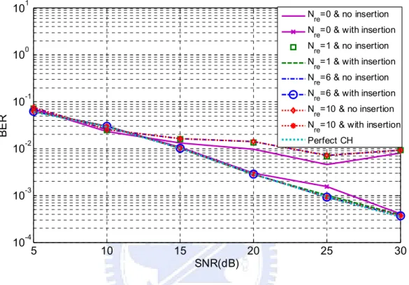
6.4.1 Results of proposed time-variant channel estimation with normalized Doppler frequency of 0.0244 ... 88

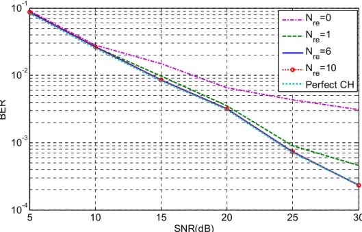
6.4.2 Results of proposed time-variant channel estimation with normalized Doppler frequency 0.1016.. 95

CHAPTER 7 CONCLUSIONS AND FUTURE WORKS... 99

List of Tables

TABLE 2-1 PARAMETERS OF THE DVB-T SYSTEM...11

TABLE 2-2 SUBCARRIER INDEX FOR CONTINUAL PILOTS... 13

TABLE 2-3 SUBCARRIER INDEX FOR TPS PILOTS... 13

TABLE 2-4 THE NUMBER OF PILOT CARRIERS FOR 2K AND 8K MODE ... 14

TABLE 6-1 PARAMETERS OF MULTIPATH FADING CHANNEL... 63

TABLE 6-2 THE WEIGHTS OF THE FIRST WEIGHTING METHOD... 79

TABLE 6-3 THE WEIGHTS OF THE SECOND WEIGHTING METHOD ... 80

TABLE 6-4 WEIGHTS USED FOR QPSK ... 80

TABLE 6-5 WEIGHTS USED FOR 16QAM ... 81

TABLE 6-6 WEIGHTS USED FOR 64QAM ... 81

TABLE 6-7 THE CHANNEL TAPS POWER FOR QPSK SCHEME ... 84

TABLE 6-8 THE CHANNEL TAPS POWER FOR 16QAM SCHEME ... 85

TABLE 6-9 THE CHANNEL TAPS POWER FOR 64QAM SCHEME ... 85

TABLE 6-10 CHANNEL TAP POWER PROFILE ... 88

List of Figures

FIGURE 2-1 OVERLAPPED AND ORTHOGONAL TRANSMISSION SPECTRUMS ... 4

FIGURE 2-2 CYCLIC PREFIX ... 5

FIGURE 2-3 CONTINUOUS-TIME OFDM BASEBAND MODULATOR... 5

FIGURE 2-4 CONTINUOUS-TIME OFDM BASEBAND DEMODULATOR ... 6

FIGURE 2-5 EQUIVALENT DISCRETE-TIME MODEL ... 7

FIGURE 2-6 BLOCK DIAGRAM OF OFDM SYSTEM... 9

FIGURE 2-7 THE TRANSMISSION SYSTEM BLOCK OF DVB-T... 10

FIGURE 2-8 SUBCARRIERS ALLOCATION ... 12

FIGURE 3-1 SCATTERED PILOTS IN DVB-T... 15

FIGURE 3-2 POLYNOMIAL INTERPOLATOR ... 17

FIGURE 3-3 INTERPOLATION IN TEMPORAL DOMAIN ... 19

FIGURE 3-4 THE INITIAL TIME-DOMAIN CHANNEL ESTIMATE... 20

FIGURE 3-5 CHANNEL TAP SEARCHING METHOD BY THE FIRST-ORDER DIFFERENTIATION METHOD... 21

FIGURE 3-6 CHANNEL TAP SEARCHING BY THRESHOLDING... 22

FIGURE 3-7 THE PROCEDURE OF THE SIGNIFICANT TAP SEARCHING METHOD... 23

FIGURE 3-8 ITERATIVE JOINT TIME AND FREQUENCY DOMAIN CHANNEL ESTIMATION ... 27

FIGURE 3-9 JOINT TIME AND FREQUENCY DOMAIN CHANNEL ESTIMATION WITH TIME DOMAIN FILTERING ... 29

FIGURE 3-10 IMPROVED JOINT TIME AND FREQUENCY DOMAIN CHANNEL ESTIMATION ... 31

FIGURE 4-1 ALIASING IN INITIAL CHANNEL ESTIMATION ... 33

FIGURE 4-2 THE SIC-LS CHANNEL ESTIMATION METHOD... 34

FIGURE 4-3 PROPOSED INITIAL CHANNEL ESTIMATION METHOD... 35

FIGURE 4-4 THE BLOCK DIAGRAM OF DATA DETECTION... 36

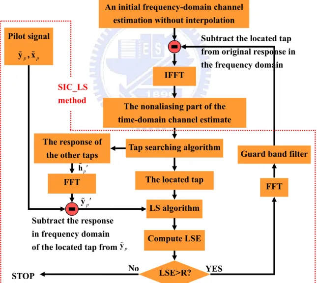
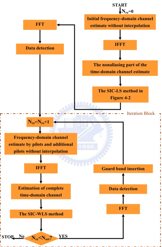
FIGURE 4-5 PROPOSED JOINT TIME AND FREQUENCY DOMAIN CHANNEL ESTIMATION METHOD... 38

FIGURE 4-8 THE PROPOSED SECOND WEIGHTING METHOD... 44

FIGURE 4-9 THE PROPOSED TIME AND FREQUENCY DOMAIN CHANNEL ESTIMATION METHOD WITH THE SIC-WLS ALGORITHM ... 45

FIGURE 5-1 ONE TIME-VARYING CHANNEL TAP... 48

FIGURE 5-2 LINEAR APPROXIMATION OF A TIME-VARIANT CHANNEL TAP... 49

FIGURE 5-3 ENTRIES NEED TO BE CONSIDERED IN (5.17) ... 55

FIGURE 5-4 THE LS TIME-VARIANT CHANNEL ESTIMATION WITH DECISIONS ... 56

FIGURE 5-5 WEIGHTING METHOD IN WLS ALGORITHM... 57

FIGURE 5-6 TIME DOMAIN TIME-VARIANT WLS CHANNEL ESTIMATION ... 59

FIGURE 6-1 AN EXAMPLE OF 6-TAP CHANNEL... 62

FIGURE 6-2 VARIATION OF CHANNEL TAPS IN FADING ENVIRONMENT ... 62

FIGURE 6-3 COMPARISON OF DIFFERENT INTERPOLATION METHODS (CHANEL A)... 64

FIGURE 6-4 COMPARISON OF DIFFERENT INTERPOLATION METHODS (CHANNEL B)... 65

FIGURE 6-5 PERFORMANCE OF THE JOINT TIME/FREQUENCY CHANNEL ESTIMATE (QPSK, CHANNEL A)... 66

FIGURE 6-6 PERFORMANCE OF THE JOINT TIME/FREQUENCY CHANNEL ESTIMATE (QPSK, CHANNEL B)... 66

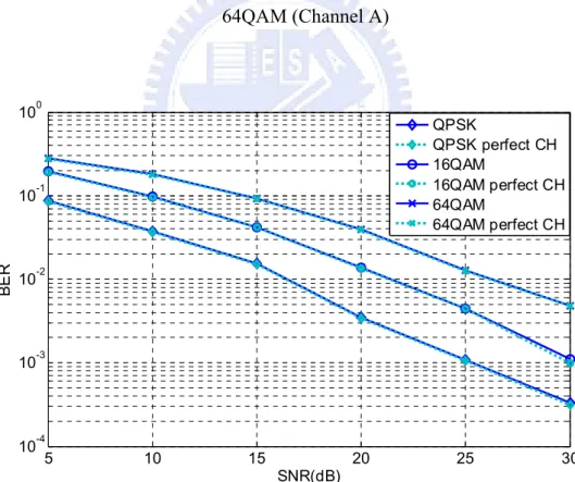
FIGURE 6-7 PERFORMANCE OF THE JOINT TIME/FREQUENCY CHANNEL ESTIMATE FOR QPSK, 16QAM, 64QAM (CHANNEL A) ... 67

FIGURE 6-8 PERFORMANCE OF THE JOINT TIME/FREQUENCY CHANNEL ESTIMATE FOR QPSK, 16QAM, 64QAM (CHANNEL B) ... 67

FIGURE 6-9 BER COMPARISON OF DIFFERENT PSEUDO PILOT SELECTION SCHEMES (WITHOUT GUARD BAND INSERTION, CHANNEL A)... 69

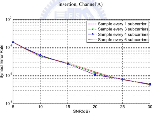
FIGURE 6-10 SER OF PSEUDO PILOTS FOR DIFFERENT PSEUDO PILOT SELECTION SCHEMES (WITHOUT GUARD BAND INSERTION, CHANNEL A) ... 69

FIGURE 6-11 BER COMPARISON OF DIFFERENT PSEUDO PILOT SELECTION SCHEMES (WITHOUT GUARD BAND INSERTION, CHANNEL A) ... 70

FIGURE 6-12 SER OF PSEUDO PILOTS FOR DIFFERENT PSEUDO PILOT SELECTION SCHEMES (WITHOUT GUARD BAND INSERTION, CHANNEL A) ... 70

FIGURE 6-13 PERFORMANCE COMPARISON FOR THE CHANNEL ESTIMATOR WITH/WITHOUT GUARD BAND INSERTION (CHANNEL A)... 71

NUMBERS OF ITERATION (SIC-LS USES PILOTS, CHANNEL A) ... 72 FIGURE 6-15 PERFORMANCE COMPARISON FOR THE CHANNEL ESTIMATOR WITH DIFFERENT

NUMBERS OF ITERATION (SIC-LS USES PILOTS, CHANNEL B) ... 72 FIGURE 6-16 PERFORMANCE COMPARISON FOR THE CHANNEL ESTIMATOR WITH QPSK,

16QAM, AND 64QAM (SIC-LS USES PILOTS, CHANNEL A)... 73 FIGURE 6-17 PERFORMANCE COMPARISON FOR THE CHANNEL ESTIMATOR WITH QPSK,

16QAM, AND 64QAM (SIC-LS USES PILOTS, CHANNEL B)... 73 FIGURE 6-18 PERFORMANCE COMPARISON FOR THE CHANNEL ESTIMATOR WITH DIFFERENT

NUMBERS OF ITERATION (SIC-LS USES ORIGINAL AND PSEUDO PILOTS,

CHANNEL A)... 74 FIGURE 6-19 PERFORMANCE COMPARISON FOR THE CHANNEL ESTIMATOR WITH DIFFERENT

NUMBERS OF ITERATION (SIC-LS USES ORIGINAL AND PSEUDO PILOTS,

CHANNEL B)... 74 FIGURE 6-20 PERFORMANCE COMPARISON FOR THE CHANNEL ESTIMATOR WITH DIFFERENT

NUMBERS OF ... 75 FIGURE 6-21 PERFORMANCE COMPARISON FOR THE CHANNEL ESTIMATOR WITH DIFFERENT

NUMBERS OF ITERATION (SIC-LS USES ORIGINAL PILOTS AND ALL DECISIONS, CHANNEL B)... 76 FIGURE 6-22 COMPARISON OF THE PROPOSED CHANNEL ESTIMATOR (NO WEIGHTING, SIC-LS

USES PILOTS, CHANNEL C)... 77 FIGURE 6-23 PERFORMANCE OF THE PROPOSED CHANNEL ESTIMATOR (NO WEIGHTING, QPSK,

16QAM, AND 64QAM, CHANNEL C) ... 78 FIGURE 6-24 PERFORMANCE OF PROPOSED CHANNEL ESTIMATION METHOD WITH WLS (THE

FIRST WEIGHTING METHOD, CHANNEL C)... 79 FIGURE 6-25 PERFORMANCE OF PROPOSED CHANNEL ESTIMATION METHOD WITH WLS (THE

SECOND WEIGHTING METHOD, CHANNEL C) ... 80 FIGURE 6-26 PERFORMANCE OF PROPOSED CHANNEL ESTIMATION METHOD WITH WLS FOR

BPSK, QPSK, 16QAM, 64QAM (CHANNEL C) ... 81 FIGURE 6-27 PERFORMANCE COMPARISON FOR PROPOSED CHANNEL ESTIMATORS WITH LS

AND WLS METHODS (BPSK, QPSK, 16QAM, 64QAM, CHANNEL C) ... 82 FIGURE 6-28 PERFORMANCE OF PROPOSED CHANNEL ESTIMATORS WITH WLS METHOD FOR

16QAM (ALL DECISIONS ARE USED, CHANNEL C) ... 83 FIGURE 6-29 PERFORMANCE OF PROPOSED CHANNEL ESTIMATORS WITH WLS METHOD FOR

FIGURE 6-30 PERFORMANCE OF PROPOSED CHANNEL ESTIMATORS WITH WLS METHOD FOR QPSK (ALL DECISIONS ARE USED, DVB-T, CHANNEL B) ... 86 FIGURE 6-31 PERFORMANCE OF PROPOSED CHANNEL ESTIMATORS WITH WLS METHOD FOR

16QAM (ALL DECISIONS ARE USED, DVB-T, CHANNEL A) ... 86 FIGURE 6-32 PERFORMANCE OF PROPOSED CHANNEL ESTIMATORS WITH WLS METHOD FOR

64QAM (ALL DECISIONS ARE USED, DVB-T, CHANNEL B) ... 87 FIGURE 6-33 PERFORMANCE OF PROPOSED TIME-VARIANT CHANNEL ESTIMATOR FOR QPSK

(SIC-LS USES PILOTS, CHANNEL A) ... 89 FIGURE 6-34 PERFORMANCE OF PROPOSED TIME-VARIANT CHANNEL ESTIMATOR FOR QPSK

(SIC-LS USES PILOTS, CHANNEL B) ... 89 FIGURE 6-35 PERFORMANCE OF PROPOSED TIME-VARIANT CHANNEL ESTIMATOR FOR QPSK

(SIC-LS USES ORIGINAL AND PSEUDO PILOTS, CHANNEL A)... 90 FIGURE 6-36 PERFORMANCE OF PROPOSED TIME-VARIANT CHANNEL ESTIMATOR FOR QPSK

(SIC-LS USES ORIGINAL AND PSEUDO PILOTS, CHANNEL B)... 91 FIGURE 6-37 PERFORMANCE OF PROPOSED TIME-VARIANT CHANNEL ESTIMATOR WITH WLS

FOR QPSK (SIC-WLS USES ORIGINAL AND PSEUDO PILOTS, CHANNEL A) ... 92 FIGURE 6-38 PERFORMANCE OF PROPOSED TIME-VARIANT CHANNEL ESTIMATOR WITH WLS

FOR QPSK (SIC-WLS USES ORIGINAL AND PSEUDO PILOTS, CHANNEL B)... 92 FIGURE 6-39 PERFORMANCE OF PROPOSED TIME-VARIANT CHANNEL ESTIMATOR WITH WLS

FOR 16QAM (SIC-WLS USES ORIGINAL AND PSEUDO PILOTS, CHANNEL A)... 93 FIGURE 6-40 PERFORMANCE OF PROPOSED TIME-VARIANT CHANNEL ESTIMATOR WITH WLS

FOR 16QAM (SIC-WLS USES ORIGINAL AND PSEUDO PILOTS, CHANNEL B)... 93 FIGURE 6-41 PERFORMANCE OF PROPOSED TIME-VARIANT CHANNEL ESTIMATOR WITH WLS

FOR 64QAM (SIC-WLS USES ORIGINAL AND PSEUDO PILOTS, CHANNEL A)... 94 FIGURE 6-42 PERFORMANCE OF PROPOSED TIME-VARIANT CHANNEL ESTIMATOR WITH WLS

FOR 64QAM (SIC-WLS USES ORIGINAL AND PSEUDO PILOTS, CHANNEL B)... 94 FIGURE 6-43 PERFORMANCE OF PROPOSED TIME-VARIANT CHANNEL ESTIMATOR WITH WLS

FOR QPSK (SIC-WLS USES ORIGINAL AND PSEUDO PILOTS, CHANNEL A) ... 96 FIGURE 6-44 PERFORMANCE OF PROPOSED TIME-VARIANT CHANNEL ESTIMATOR WITH WLS

FOR QPSK (SIC-WLS USES ORIGINAL AND PSEUDO PILOTS, CHANNEL B)... 96 FIGURE 6-45 PERFORMANCE OF PROPOSED TIME-VARIANT CHANNEL ESTIMATOR WITH WLS

FOR 16QAM (SIC-WLS USES ORIGINAL AND PSEUDO PILOTS, CHANNEL A)... 97 FIGURE 6-46 PERFORMANCE OF PROPOSED TIME-VARIANT CHANNEL ESTIMATOR WITH WLS

FOR 16QAM (SIC-WLS USES ORIGINAL AND PSEUDO PILOTS, CHANNEL B)... 97 FIGURE 6-47 PERFORMANCE OF PROPOSED TIME-VARIANT CHANNEL ESTIMATOR WITH WLS

FOR 64QAM (SIC-WLS USES ORIGINAL AND PSEUDO PILOTS, CHANNEL A)... 98 FIGURE 6-48 PERFORMANCE OF PROPOSED TIME-VARIANT CHANNEL ESTIMATOR WITH WLS

Chapter 1

Introduction

Orthogonal Frequency Division Multiplexing (OFDM) has been an important modulation technique in wireless communication. The distinct advantage of OFDM is that it can significantly increase the spectrum efficiency. Also, it can effectively combat the multipath channel fading, and allow multiple users to access the channel at the same time. The OFDM technique has been successfully used in many commercial systems such as wireless local area network (LAN), digital video broadcasting (DVB), WiMAX etc.

Due to multipath propagation, the channel is often fading in wireless systems. In order to recover the transmitted signals in the receiver, accurate channel estimation is essential. For OFDM systems, pilot subcarriers are frequently inserted in the OFDM symbols to aid the channel estimation. Since the inserted pilots will reduce the transmission bandwidth, the number of pilots is usually kept to a minimum. As a result, the channel estimation becomes challenging in some scenarios. In this thesis, we consider the channel estimation problem in the DVB-terrestrial (DVB-T) system. This is a standardized system for digital terrestrial television broadcasting and has been adopted in Taiwan and many other countries. The DVB-T system transmits and receives compressed digital audio, video and other data in an MPEG transport stream and use OFDM as its modulation technique.

Channel estimation has been considered in the literature [2 ]-[4]. To obtain satisfactory performance, the implementation complexity is generally high. This is because the pilot density in DVB-T system is 1/12 which is not enough to conduct the channel estimation

accurately. As a result, we have to cluster four OFDM symbols to make the density up to 1/3, and this significantly increase the memory size and subsequently the implementation complexity. Also, in high-mobility environments, the channel responses of four consecutive OFDM symbols will not be the same, the clustering approach will not work. We propose new algorithms to use the limited pilots to conduct the channel estimation effectively. Conventional approaches conduct the channel estimation in the frequency domain and perform poorly when the pilot density is low. In this thesis, we propose a new joint time/frequency domain channel estimation method to overcome the problem. Using the proposed method, we needs only one OFDM symbol to achieve precise channel estimation.

In the high-mobility wireless communication environments, the channel may become time variant even in one OFDM symbol. This will cause the intercarrier interference (ICI) degrading the receiver performance. Many ICI mitigation methods have been proposed [7], [9]-[14]. However, all algorithms require the knowledge of the channel state information. Although some estimation methods for time-variant channel have been proposed [3], [6], [8], [14] there is still much room for performance improvement. We extend the joint time and frequency domain channel estimator proposed for the time-invariant channel to the time-variant channel scenario. It is shown that the estimation performance can be greatly enhanced.

This thesis is organized as follows. First, we will briefly describe the OFDM technique and the wireless communication system of DVB-T in Chapter 2. Then, we will describe the existing channel estimation method in Chapter 3. In Chapter 4, we propose new joint time and frequency domain channel estimators for systems with uniform distributed pilot-subcarriers such as the DVB-T system. In Chapter 5, we propose new joint time and frequency domain channel estimator for time-variant channel in the DVB-T system. Then we evaluate the performance of the proposed algorithms using the simulations and the results are reported in

Chapter 2

Introduction to OFDM and DVB-T Systems

2.1 OFDM system

As the data rate of a communication system becomes higher and higher, the symbol duration becomes smaller and smaller. The system then becomes more susceptible to loss of information due to impulse noise, signal reflections and other impairments. A remedy for this problem is to split a higher data-rate stream into lower data-rate sub-streams, and this is equivalently to divide the available wideband channel into narrowband subchannels. Each data stream is transmitted with a subcarrier in a subchannel. This approach is called Frequency division multiplexing (FDM). In FDM, the data to be transmitted do not have to be divided equally nor do they have to originate from the same information source.

FDM offers an advantage over single-carrier modulation in terms of the immunity to the narrowband frequency interference. Since the bandwidth of each subchannel is narrow, each transmitted signal in the subchannel experiences flat channel fading. Thus, channel equalization is simplified to a one-tap frequency domain equalizer. And the narrowband interference will only affect one of the frequency subbands. Since the data rate for each subcarrier is lower, the symbol period will be longer, adding some additional immunity to impulse noise and other impairments.

In OFDM systems, these subcarriers are designed orthogonal to allow spectrum overlapping, achieving a high spectral efficiency. As long as the orthogonality is maintained, we can recover each individual subcarrier’s signal despite the overlapped spectrum. Figure 2-1 shows the overlapped spectrums of OFDM modulated signals. With the sinc-shaped spectrums, we can guarantee the spectrum of one subcarrier is nulled at other subcarriers’

frequencies. The subcarrier spacing between two neighbor subcarrier can be calculated

as f W 1

N T

Δ = = . Where W is the bandwidth, N is the number of subcarriers, and T is the symbol period.

Figure 2-1 Overlapped and orthogonal transmission spectrums

A major problem in most wireless systems are the presence of the multipath channel causing the intersymbol interference (ISI) effect. To combat the problem, a cyclic prefix (CP) whose size is larger than the maximum channel delay spread, is added in front of each OFDM symbol. Due to the CP, the ISI is avoided and the transmitted signal becomes partially periodic, and the effect of the linear convolution with a multipath channel can be translated to a circular convolution at the receiver. Thanks to circular convolution, in the frequency domain the channel effect is simplified to a point-to-point multiplication of the data symbol and channel frequency response. Thus, only a one-tap frequency domain equalizer is required. The generation of the CP is shown in Figure 2-2.

N

subcarriers

f

W f N Δ =

……

……

Figure 2-2 Cyclic prefix

2.1.1 Continuous-time OFDM signal model

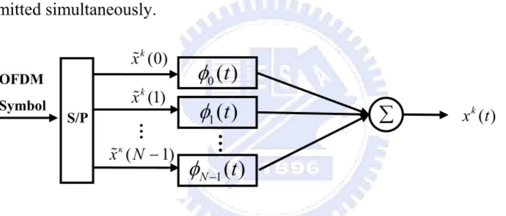
A typical continuous-time OFDM baseband modulator is shown in Figure 2-3. The input data steam is first split into parallel streams which modulate different subcarriers, and then transmitted simultaneously.

Figure 2-3 Continuous-time OFDM baseband modulator The i -th modulating subcarrier ( )φ_i t can be represented as

2 ( ) , 0 ( ) 0, g j i t T T s i t e t T otherwise π

φ

− ⎧⎪ _{≤ ≤} = ⎨ ⎪⎩ ，Ts = + (2.1) T Tg

where T is the symbol duration excluding CP, T is the length of CP and _g T is the total _s symbol duration. _{x i is the transmitted signal, which is a complex number from a set of} k( ) signal constellation points, at the i -th subcarrier for the k-th OFDM symbol. The modulated baseband signal for the k-th OFDM symbol can be expressed as

1 0 ( ) N ( ) ( ) k k i s i x t − x i φ t kT = =

∑

− (2.2)

where N is the number of subcarriers. When an infinite sequence of OFDM symbols is

CP

OFDM symbol Ts Tg T

∑

(0) k x (1) k x ( 1) k x N − OFDM Symbol S/P 0

( )

t

φ

1

( )

t

φ

1

( )

N

t

φ

₋ … _{x t}k( )

…

considered, the transmit signal can be represented as 1 0 ( ) k( ) N k( ) ( ) i s k k i x t ∞ x t ∞ − x i φ t kT =−∞ =−∞ = =

∑

=

∑ ∑

− (2.3) And, the received signal y t can be expressed as ( )

( ) ( , ) ( ) ( )

y t h t τ x t τ τd w t

∞ −∞

=

_∫

− + (2.4) where h t( , )τ denotes the time-variant channel impulse response at time t , and w t is the ( ) additive white complex Gaussian noise.

Figure 2-4 Continuous-time OFDM baseband demodulator

A typical continuous-time OFDM baseband demodulator is shown in Figure 2-4, in which ( )ψ_i t denotes the matched filter for the i -th subcarrier.

2 1 , 0 ( ) 0, j it s i e t T t T otherwise π ψ _{= ⎨}⎧⎪ ≤ ≤ ⎪⎩ ，Ts = + (2.5) T Tg where T is the symbol duration excluding CP, T is the length of CP and _g T is the total _s symbol duration. _{y i is the demodulated signal at} k( ) _{i -th subcarrier for the k-th symbol.}

2.1.2 Discrete-time OFDM system model

Consider a particular OFDM symbol, the modulated baseband signal is given by

2 1 0 1 ( ) , 0 j it N T i i x t x e t T T π − = =

∑

≤ ≤ (2.6) P/S 1

( )

t

ψ

1

( )

N

t

ψ

₋ ( ) y t

…

(1) i y ( 1) i y N− (0) i y 0

( )

t

ψ

Lett=nT_d, in which T_d T N

= is the sampling period. Equation (2.6) can be rewritten as

2 1 0 1 [ ] ( ) | , 0 1 d j in N T t nT i i x n x t x e n N N π − = = = =

∑

≤ ≤ − (2.7)

For a noise-free system, we can recover the transmit symbols from (2.7) as

y

i

2 1 0 1 [ ] j in N N i n y x n e N π − − = =

∑

(2.8)

From (2.7) and (2.8), it is simple to see that modulation/demodulation in OFDM systems can be conducted by inverse discrete Fourier transform (IDFT) and discrete Fourier transform (DFT). In practice, IDFT/DFT is implemented with inverse fast Fourier transform (FFT)/fast Fourier Transform (IFFT). Figure 2-5 shows the OFDM modulator/demodulator.

Figure 2-5 Equivalent discrete-time model

The modulation operation can then be described as follows. In the transmitter, the data stream is grouped in blocks of data symbols, called OFDM symbols. Then an IDFT is

performed for each data symbol block, and a CP of length T is added. Passing the resultant _g signal through a time-variant multipath channel, we have the received signal as

1 0 ( ) L ( , ) ( )_N ( ) l y n − h n l x n l w n = =

∑

− + (2.9)

where h n l is the ( , ) l-th channel path at time instant n, L is the number of channel taps, ( . )_N represents a cyclic shift in the base of N , and w n is sampled additive white ( )

( ) x n P/S

+

( 1) i X N−

( , )

h n l

…

IDFT

(0) i X

…

CP ( ) y n ( ) w n S/P

IDFT

(0) i Y

…

CP (1) i X ( 1) i Y N−

complex Gaussion noise with variance _σ2_{. In the receiver, the received sequence is first}

split into blocks, and the CP associated with each block is removed. Then, a DFT is performed for each symbol to recover the original data symbols.

As mentioned, carriers in subbands experience flat fading, which reduces equalization to a single complex multiplication per carrier. A matrix equivalent model can be used to obtain a more compact expression. For a single OFDM symbol, the received signal can be represented as 0 00 0 1 11 1 2 22 2 1 ( 1)( 1) 1

0

0

0

0

0

0

0

0

0

0

0

0

C C C C N N N N

y

h

x

y

h

x

y

h

x

y

₋

h

_{− −}

x

₋

⎡

⎤

⎡

⎤

⎡

⎤

⎢

⎥

⎢

⎥

⎢

⎥

⎢

⎥

⎢

⎥

⎢

⎥

⎢

⎥

⎢

⎥

=

⎢

⎥

+

⎢

⎥

⎢

⎥

⎢

⎥

⎢

⎥

⎢

⎥

⎢

⎥

⎢

⎥

⎢

⎥

⎢

⎥

⎣

⎦

⎣

⎦

⎣

⎦

w

(2.10) where [ , ,_{0 1 1}] c T N

x x x ₋ is the frequency domain transmitted data vector, [ , ,_{0 1 1}] c

T N

y y y ₋ is

the frequency domain received data vector, W is the AWGN noise vector, and

00 11 ( 1)( 1)

{[ , , ]}

c c

N N

diag h h h _{− −} are the channel frequency response.

2.1.3 Complete OFDM system

Figure 2-6 shows the block diagram of a complete OFDM system, where the upper path is the transmitter chain, and the lower path is the receiver chain. First, input data are encoded by the channel encoder. The encoded bits are then interleaved and mapped onto QAM constellations. After that, each block of input QAM symbols is modulated onto subcarriers by the IFFT operation, and then a CP is added to form an OFDM symbol. Finally, the baseband OFDM signal is passed to the digital-to-analog (D/A) converter and the RF circuit for transmission. In the receiver, the received signal is first sampled by an analog-to-digital (A/D)

converter, and various receiver operations such as synchronization, channel estimation, demapping and decoding are conducted.

Figure 2-6 Block diagram of OFDM system

2.2 Introduction to DVB-T system

DVB-T uses the coded-OFDM transmission technique; it allows the receiver to cope with strong multipath situations. Within a geographical area, DVB-T also allows a single-frequency networks (SFN) operation, A single-frequency networks is a broadcast network where several transmitters simultaneously send the same signal over the same frequency channel. Coding & Interleaver Mapper (Modulator) IFFT(OFDM Modulator) CP Adder D/A Converter Decoding & Deinterleaver Demapper (Demodulator) CP Remover A/D Converter Channel & AWGN Noise FFT(OFDM Demodulator) Output Data Channel Estimation Synchronization Transmitted Data

2.2.1 System blocks of DVB-T

Figure 2-7 shows the block diagram of a DVB-T transmitter. The operations conducted in the transmitter include randomization, outer encoding, outer interleaving, inner encoding, inner interleaving, mapping, frame adaptation, OFDM modulation, and guard interval insertion.

Figure 2-7 The Transmission system block of DVB-T

And the operations conducted in a DVB-T receiver should include time and frequency synchronization, CP removal, OFDM demodulation, frequency equalization, demapping , inner deinterleaving, inner decoding, outer deinterleaving, outer decoding, demultiplexing and source decoding.

2.2.2 The system parameters of DVB-T

A DVB-T channel have a bandwidth of 8,7 or 6MHz. The sampling period is 7 48μs,

1 8μs, or 7

64μs.There are two different operating modes : 2k and 8k mode. The 2K mode is to split

Randomiztion for energy dispersal Outer Encoder Out Interleaver Inner Encoder Inner Interleaver Mapper Frame Adaptation IFFT CP Adder MPEG-2 Data Stream Add TPS & Pilots Channel & AWGN Noise D/A Converter Guard Band Insertion

the bandwidth into 2048 subchannels. It conducts 2048-point IFFT and FFT operations. The actual number of subchannels for data transmission is 1705. The 8K mode is to split the bandwidth into 8192 subchannels. It conducts 8192-point IFFT and FFT operations. The actual number of subchannels for data transmission is 6817. The 2K mode has greater subcarrier spacing which is about 4KHz. This is also indicates that the symbol period is shorter. The subcarrier spacing for the 8K mode is about 1KHz. The CP size can be chosen as

1 4 or 1 8 or 1 16 or 1

32 of the symbol length.

Table 2-1 Parameters of the DVB-T system

DVB-T offers three different modulation schemes which are QPSK, 16QAM, and 64QAM, and it adopts gray mapping for modulation. System parameters for the DVB-T system are summarized in Table 2-1.

2.2.3 The frame structure of DVB-T

Under the 2K mode, a frame is constituted by 68 OFDM symbols. And a super OFDM frame can be constituted by 4 OFDM frames. An OFDM not only transmits information data, but also training data and system parameters which include scattered pilots, continual pilots, and transmission parameter signaling (TPS) data. The pilot signals are used for synchronization and channel estimation.

pilots, and TPC data.

Figure 2-8 Subcarriers allocation

Within each symbol, a scattered pilot is inserted every 12 carriers. Each scattered pilot jumps forward by three carrier positions in the next symbol. So the scattered pilot will be on the same subcarrier positions every four OFDM symbols. The power level of a scattered pilot

is boosted by4

3, and the BPSK data are sent as scattered pilots. The phase of a BPSK signal, either 0 orπ , is decided by the Pseudo Random Binary Sequence (PRBS). The scattered pilots are mainly used to conduction channel estimation. Since the pilots are scattered, the complete channel response must be obtained using interpolation.

Unlike scattered pilots, the positions of the continual pilots are fixed. The power level of

the continual pilot is also boosted by4

3, and the BPSK data are sent as continual pilots. The phase of a BPSK signal, either 0 orπ , is also determined by the Pseudo Random Binary Sequence (PRBS). The continual pilots are mainly used for channel estimation and frequency synchronization. The frequency synchronization is also referred to as automatic frequency

Scattered pilot subcarrier Data subcarrier

...

Subcarrier

TPS subcarrier

Continual pilot subcarrier

OFDM Symbol

positions for the continuous pilots are given in Table 2-2.

Table 2-2 Subcarrier index for continual pilots

TPS data give information about the current transmission status, including the frame number, QAM size, coding rate, CP size etc. The TPS data are sent through TPS pilots whose locations are given in Table 2-3. The complete TPS information is broadcasted over 68 symbols in one OFDM frame and carried in 68 bits. To lower the error rate, DBPSK is used for the modulation scheme.

Table 2-3 Subcarrier index for TPS pilots

Table 2-4 shows the number of subcarriers allocated for data, scattered pilots, continual pilots, and TPS pilots.

Mode

Carriers 2K Mode 8K Mode total carriers 2048 8192 active carriers 1705 6817 scattered carriers 142/131 568/524 continual carriers 45 177

TPS carriers 17 68

Chapter 3

Joint Time and Frequency Domain Channel Estimation

Consider a specific subcarrier of subcarrier index i in an OFDM symbol. We

have

y

_i

=

h x

_{i i}

+

w

_i , where

y

_i is the frequency-domain received signal,

x

_i is the frequency-domain transmitted signal,

h

iis the channel frequency response, and

w

iis the

corresponding AWGN noise. It is apparent that if both x and _i y are known, _i h can then be _i

estimated. Let y_p = h x_{p p} + w_p where the subscript denotes the subcarrier in a pilot position. We can estimate the channel response in the pilot position, denoted by hˆ_p, as:

ˆ

p p p

y

h

x

=

_(3.1) In the DVB-T system, there is a scattered pilot every 12 subcarriers, as shown in Figure 3-1.

Figure 3-1 Scattered pilots in DVB-T

To obtain the channel responses in data subcarriers, we need to conduct interpolation. In the next two sections, we will describe two simple interpolation techniques, one-dimensional

……

OFDM Symbol Pilot subcarrier Data subcarrier

...

Subcarrier

and two-dimensional interpolation methods. If the number of pilot subcarriers is not sufficiently large, the interpolated result may not be satisfactory. In this case, the time-domain channel estimation requiring fewer pilots may be used. In the last section, we will describe a recently developed method, a joint time and frequency domain channel estimation method.

3.1 Interpolation methods

The classical approach for channel interpolation is to construct a polynomial interpolator fitting responses in known samples. The polynomial interpolator can be formulated in various ways, such as the power series, Lagrange interpolation and Newton interpolation. These various forms are mathematically equivalent and can be transformed from one to another. We will use the power series as our polynomial interpolator. Assume that there are some samples

available, denoted as

{

x f( ), ( ), , (_o x f₁ x f_N)}, where ( )x f is the amplitude of the signal _n ( )

x f at frequency f . The polynomial with order_n N , passing through the N+1 known samples, can be written in a power series form as

2

0 1 2

( ) ( ) N

N N

x f =P f =e +e f +e f + +e f (3.2)

where ( )P f is a polynomial of order _N N, and e s are the polynomial coefficients. An _k' example of the polynomial interpolator is shown in Figure 3-2. As we can see from Figure 3-2 that the fitted polynomial is unique.

f0 f1 f2 f4 f5 f6 f7

x(f)

Figure 3-2 Polynomial interpolator

For all the signals in pilot subcarriers, we can write (3.2) into a matrix form.

1 1 1 1 1 1 1 1 2 1 0 2 1 1 2 1 1

(

)

₁

(

)

₁

(

)

1

o o o o M M M M N m m m m N m m m m N m _{m m m} N

f

f

f

x f

e

x f

f

f

f

e

x f

₋

_f

_f

_f

e

− − − − − − −

⎡

⎤

⎡

⎤

_⎢

_⎥

⎡

⎤

⎢

⎥

_⎢

_⎥

⎢

⎥

⎢

⎥

_{= ⎢}

_⎥

⎢

⎥

⎢

⎥

_⎢

_⎥

⎢

⎥

⎢

⎥

_⎢

⎢

⎥

⎥ ⎣

⎦

⎣

_{⎦ ⎣}

_⎦

(3.3)

The matrix form can be expressed as:

x = Fe

(3.4) where

x

=

{

x f

(

m₀

), (

x f

m₁

),

, (

x f

m_M−1

)

}

T , ,0mi ≤ ≤i M− and M is the number of 1

pilot signals, F is the matrix at the right hand side of (3.3), e=

{

e e₀, , ,₁ e_N−1

}

T is the polynomial coefficients, and N is the order of polynomial interpolator. Note thatN is usually small since the computational complexity of the interpolation is proportional to N . In practice, the linear (N=1) and quadratic (N =2) and cubic (N=3) interpolator is often used.

Since M is usually larger than N , the system in (3.4) is overdetermined. So, the polynomial coefficients can be solved by the least-squares (LS) algorithm. With the LS algorithm [5], we then have

H -1 H

e = (F F) F x

(3.5) The simplest polynomial interpolator is the first-order (i.e, the linear) polynomial interpolator. However, the performance is usually not satisfactory. The cubic interpolator being a third-order polynomial interpolator is widely used in real-world applications. It can have better performance while the computational complexity is acceptable.

The one dimensional linear interpolation method uses one OFDM symbol and simply conducts the interpolation for the channel responses in data subcarriers. In order to obtain better performance, we can change the linear interpolation to cubic interpolation in the one dimensional interpolation method. We will discuss the performance of the linear and cubic interpolation methods in the simulation chapter.

The main advantage of the one-dimensional interpolation approach is that it needs only one OFDM symbol and the requirement for the memory size is small. Also, the computational complexity of the one-dimensional linear interpolation is low. However, due to the low density of scattered pilots, this method cannot achieve satisfactory performance in general. To solve this problem, we will introduce the two-dimensional linear interpolation method below.

Since the positions of the scattered pilots are the same for every 4 OFDM symbols, we can conduct interpolation in the temporal domain. The two-dimensional interpolation method uses consecutive OFDM symbols to conduct interpolation both in the frequency and temporal domains. With this approach, the pilot density can be effectively increased. Figure 3-3 shows the linear interpolation in temporal domain. In the figure, the channel responses of the middle OFDM symbol are those we want to estimate (the dotted block). We first interpolate linearly the responses in the temporal domain. The interpolated responses can be seen as pseudo pilots which can be used in the interpolation in the frequency domain. As we can see, the pilot

density is increased from 1 12 to

1 3.

Figure 3-3 Interpolation in temporal domain

Since the scattered pilot density is raised to1

3, we can obtain the channel responses in frequency domain more accurately. The two-dimensional interpolation method is better than the one-dimensional interpolation method when the channel responses are highly variant. But the two-dimensional interpolation method needs 7 OFDM symbols to conduct interpolation in both frequency domain and temporal domain. The computational complexity is high and the required memory is large.

In order to obtain better performance, we can also use the cubic interpolation to replace the linear interpolation. The performance comparison of the one-dimensional interpolation methods and the two-dimensional interpolation methods will be shown in the simulation chapter. We will also discuss the performance comparison of the linear and cubic interpolation methods in the simulation chapter.

3.2 Joint time and frequency domain channel estimation

Due to limited pilot signals, channel estimation using the frequency domain interpolation will be degraded when the channel delay spread is large. In this case, the interpolation method may not be able to recover the frequency response, even with the two-dimensional

OFDM Symbol

...

Subcarrier

Pilot subcarrier Data subcarrier Pseudo pilot subcarrier

interpolation method.

In typical wireless channels, the delay spread may be large, but the number of non-zero taps is small. Since the taps of channel are usually fewer, the unknowns of channel responses in time domain are less than those we need to estimate in the frequency domain. As a result, it is possible for the time-domain approach to have better performance under the same number of pilots. In this subsection, we will describe a newly developed joint time/frequency domain channel estimation method [3], [4].

The first step of the method is to use a two-dimensional interpolation method, with the linear interpolation in the time domain and cubic interpolation in the frequency domain, to obtain the channel responses in the frequency domain. Then, we transform the channel response into the time-domain to obtain the time-domain channel response. One example of the time-domain channel responses is shown in Figure 3-4.

0 20 40 60 80 100 0 0.1 0.2 0.3 0.4 0.5 0.6 0.7 0.8 Tap Delay (Ts) m a gn itud e

Initial channel estimate in time domain

Figure 3-4 The initial time-domain channel estimate

As we can see, there are only a few significant channel taps. Then, the method locates those taps and estimates their values. The tap searching and the magnitude estimation

algorithms are described in following 3.2.1 and 3.2.2. A more efficient recursive procedure is finally described in 3.3.3.

3.2.1 Tap searching algorithm

As we can see from Figure 3-4, there is a low-pass signal embedded in the channel response. So some fake taps will occur near the significant taps. In this subsection, we outline an iterative method that can solve the problem.

If we take a first-order differentiation to the channel response, the low-pass signal will be

removed. The differentiation operation is given byd k[ ]=h kˆ[ + −1] h kˆ[ ]( ˆ[h k+ , ˆ[ ]1] h k is the tap value of different taps). With a threshold, we can find the significant tap by this method. However, if there are consecutive significant taps, the operation can not find all the taps.

Figure 3-5 Channel tap searching method by the first-order differentiation method

Another method to find the taps is simply to compare the magnitude of a tap with a threshold. If it is larger than the threshold, the tap is deemed as a peak (significant tap). Apparently, some fake taps occurring near the significant taps will also be detected as significant taps.

Channel tap found by the first-order differention method Unfound tap by the

Figure 3-6 Channel tap searching by thresholding

We can combine the aforementioned two methods to obtain a more reliable method. The idea is to locate the taps in an iterative manner, rather than in one short. Figure 3-7 shows the iterative procedure. First, locate significant the channel taps by the first-order differentiation method (Figure 3-7-(a)) with a high threshold value (Figure 3-7-(b)). In this case, smaller or consecutive significant taps may not be detected. Using the estimation method described in the next subsection, we can estimate the magnitude of those located taps. Then, subtract the channel response formed by the located channel taps from the original channel response (Note that this operation is conducted in the frequency domain). We can then have a residual channel response. Thus, we can transform the response to the time-domain and conduct the tap searching algorithm again (the threshold can be made smaller). Repeat this process until no significant taps are detected.

Unfound channel tap by thresholding Channel tap found by thresholding Threshold

Figure 3-7 The procedure of the significant tap searching method

3.2.2 LS channel estimator

For a subcarrier of subcarrier index i in a particular OFDM symbol, the signal

transmitted and passed through the channel can be expressed as

y

i

=

h x

i i

+

w

i. Let N be

the FFT size. We can write the equation for all subcarriers. We have

0 00 0 1 11 1 2 22 2 1 ( 1)( 1) 1

0

0

0

0

0

0

0

0

0

0

0

0

C C C C N N N N

y

h

x

y

h

x

y

h

x

y

₋

h

_{− −}

x

₋

⎡

⎤

⎡

⎤

⎡

⎤

⎢

⎥

⎢

⎥

⎢

⎥

⎢

⎥

⎢

⎥

⎢

⎥

⎢

⎥

⎢

⎥

=

⎢

⎥

+

⎢

⎥

⎢

⎥

⎢

⎥

⎢

⎥

⎢

⎥

⎢

⎥

⎢

⎥

⎢

⎥

⎢

⎥

⎣

⎦

⎣

⎦

⎣

⎦

w

(2.10)

The LS channel estimator minimize the following squared errors:

Channel taps left after subtracting the detected taps

(b)

(c)

Unfound tap by first-order differention Channel tap that we want to remove found by the first-order differention and thresholding (The ones to be subtracted) Channel tap found by the

first-order differention

Threshold

Channel tap found by first-order differention Unfound tap by first-order differention

2

ˆ

LS

−

y H x

(3.6) Where y =

[

y y₀, ,...₁ y_N−₁

]

T is the frequency domain received signal vector,

[

0

, ,...

1 1

]

T N

x x

x

−

=

x

is the frequency domain transmitted signal vector. Using pilot subcarriers, we can have the LS channel estimator minimize the following squared errors:

2 p,LS p p

y

− H

∧

x

(3.7) where ₀

,

₁

,...

_{M 1} T p

= ⎣

⎡

y

m

y

m

y

m ₋

⎤

⎦

y

is the frequency domain received vector on pilot locations,

x

p

= ⎣

⎡

x

m₀

,

x

m₁

,...

x

m_M−1

⎤

⎦

T is the frequency domain transmitted pilot signal

vector (m_i,0≤ ≤i M − is pilot location and M is the number of pilots). With the LS 1 algorithm, we then have

(

_H

)

-1 _H

p,LS _{p p p p}

∧

H

= x x

x

y

_(3.8) The LS channel estimator also has a time-domain version. The signal transmitted and

passed through the channel can be expressed as

y

_i

=

x

_i

gh

+

w

_iwhere

y

_i is the frequency domain received signal,

x

i is the frequency domain transmitted signal, h is the channel

response in time domain, g is a row of the DFT matrix,

w

i is noise. Considering all pilot

subcarriers, we can have Let 0 1 2 1

0

0

0

0

0

0

0

0

0

0

0

0

M m m D,p m m

x

x

x

x

−

⎡

⎤

⎢

⎥

⎢

⎥

⎢

⎥

=

⎢

⎥

⎢

⎥

⎢

⎥

⎣

⎦

X

(3.9)

0 0 0 0 _{1 1 1} 1 2 2 2 2 1 _{1 1 1} *0 *1 *( 1) 2 2 2 *0 *1 *( 1) 2 2 2 *0 *1 *( 1) 2 2 2 *0 *1 *( 1) 2 2 2 M _{M M M} m m m L j j j N N N m _{m m m L} j j j N N N m m m m L j j j D,p m _{N N N} m _{m m m L} j j j N N N e e e y y e e e y e e e y e e e π π π π π π π π π π π π − _{− − −} − − − − − − − − − − − − − − − − ⎡ ⎢ ⎡ ⎤ _⎢ ⎢ ⎥ _⎢ ⎢ ⎥ _⎢ ⎢ _{⎥ = ⎢} ⎢ ⎥ _⎢ ⎢ ⎥ _⎢ ⎢ ⎥ ⎣ ⎦ ⎣ X 0 1 1 L h h h ₋ ⎤ ⎥ ⎥ ⎡ ⎤ ⎥ ⎢ ⎥ ⎥ ⎢ ⎥ + ⎥ ⎢ ⎥ ⎥ ⎢ ⎥ ⎥ ⎣ ⎦ ⎢ ⎥ ⎢ ⎥ ⎦ w _(3.10)

Then, we can have a similar formulation as that in (3.7). The LS channel estimator in time domain minimizes the following squared errors:

2 , LS p D p ∧

−

y

X

G h

(3.11) where G is the DFT matrix. And the LS solution to the time domain LS channel estimation is then:

(

_{H H}

)

-1 _{H H} LS _{D,p D,p D,p p} ∧

=

h

G X

X G

G X

y

(3.12) where X_D,pis a diagonal matrix containing pilot signals. The time-domain LS method

requires _{O L( )}3 _{arithmetic operations where L is the maximum channel delay spread. If L}

is large, the required computational complexity is high. If we only consider L significant taps in whichL is much less thanL, the computational complexity can be reduced. For example, if we only consider h and ₀ h_L−1, we only have to use the first and last column of

G and the matrix to inverse in (3.11) becomes a 2 2× matrix. We then have

(3.13)

,

p D p

+

y = X G'h w

(3.14) where G' is a reduced DFT matrix contain the columns within the dotted block shown in (3.13). In an extreme case, we can only estimate a channel tap at one iteration. The computational complexity is further reduced since the DFT matrix is degenerated to a vector.

3.2.3 Iterative joint time and frequency domain channel estimation

In previous subsections, we have described a low-complexity yet high-performance channel estimator. We called this a joint time and frequency domain channel estimator. The estimation flowchart is shown in Figure 3-8, and the related procedure is summarized as follows: (Notice LSE represents LS error and R represents the LSE threshold)

0 0 0 0 1 1 1 1 2 2 2 2 1 _{1 1 1} *0 *1 *( 1) 2 2 2 *0 *1 *( 1) 2 2 2 *0 *1 *( 1) 2 2 2 *0 *1 *( 1) 2 2 2 M _{M M M} m m m L j j j N N N m _{m m m L} j j j N N N m m m m L j j j D,p m _{N N N} m _{m m m L} j j j N N N e e e y y e e e y e e e y e e e π π π π π π π π π π π π − _{− − −} − − − − − − − − − − − − − − − − ⎡ ⎢ ⎡ ⎤ _⎢ ⎢ ⎥ _⎢ ⎢ ⎥ _⎢ ⎢ _{⎥ = ⎢} ⎢ ⎥ _⎢ ⎢ ⎥ _⎢ ⎢ ⎥ ⎣ ⎦ ⎣ X 0 1 1 L h h h ₋ ⎤ ⎥ ⎥ ⎡ ⎤ ⎥ ⎢ ⎥ ⎥ ⎢ ⎥ + ⎥ ⎢ ⎥ ⎥ ⎢ ⎥ ⎥ ⎣ ⎦ ⎢ ⎥ ⎢ ⎥ ⎦ w

Figure 3-8 Iterative joint time and frequency domain channel estimation

STEP 1: Use the two-dimensional interpolation method to obtain the initial frequency-domain channel estimate.

STEP 2: Conduct the IFFT of the frequency domain channel estimate to obtain the time-domain channel estimate.

STEP 3: Find the tap with the maximum value (the threshold of tap search is iteration dependent) and use the LS algorithm to estimate the response of the maximum tap.

STEP 4: Compute the least-squares error (LSE) of all located and estimated taps with a

threshold (LSE threshold). If the LSE is greater than the LSE threshold, Conduct the FFT of the channel response estimated in the time domain (with the located and estimated taps) and subtract the resultant response from the

Interpolated frequency domain channel estimate

IFFT

Tap searching algorithm LS algorithm

Guard band filter

FFT

LSE>R? Compute LSE

STOP

Locate the tap Find the tap value

Subtract the located tap from original response in frequency domain

Force guard band to zero

YES No

channel response estimated in the previous iteration. Note that we have to null the responses in the guard band region. Then, go to STEP 2. If the LSE is smaller than the LSE threshold, stop the iteration.

Note that the LSE is a good indicator telling us when to stop the searching. In other words, it can avoid the redundant operations and reduce the computational complexity for the LS algorithm. In mobile environments, the channel tap positions may change with time suddenly. The LSE can also help us to check whether the channel taps’ positions have changed or not. The iterative operation not only locates the channel taps more precisely, but also requires less computational complexity for the LS algorithm.

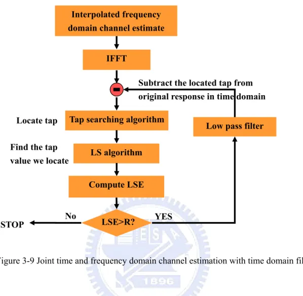
As seen, an FFT/IFFT operation is required for each iteration and this will increase the computational complexity significantly. This can be remedied with the following approach. The main idea is to transfer the response-subtraction operation in the frequency domain to the time domain. Note that the operation conducted in the frequency domain is windowing and subtraction, which can be transferred into convolution and subtraction in the time domain. The function to be convolved is the sinc filter. In practice, the sinc filter may be difficult to implement. So, we may replace it by some lowpass filter. Since the number of detected taps is expected to be small, the required computational complexity of the convolution operation will not be significant. The modified flowchart of the modified scheme is shown in Figure 3-9.

Figure 3-9 Joint time and frequency domain channel estimation with time domain filtering

3.2.4 Improved joint time and frequency domain channel estimation

One problem associated with method described above is that the estimation of a significant tap may be affected by the other significant taps. An improved method was then proposed in [4]. The main idea is to conduct a re-estimation for all significant taps. After all the taps has been estimated, we can conduct the re-estimation of one tap by subtracting the channel response contributed from the other taps and using the LS method shown above. Using the approach, the estimation accuracy can be improved. The procedure is summarized below. Figure 3-10 show the flowchart of the method. Note that the channel taps can be re-estimated more than one time until the satisfactory result is obtained.

Interpolated frequency domain channel estimate

IFFT

Tap searching algorithm

LS algorithm

Low pass filter

Compute LSE Locate tap

Find the tap value we locate

Subtract the located tap from original response in time domain

LSE>R?

STEP 1: With the channel estimation method described above, we get L significant

taps. We can order

h

k’s and start from the maximum one.

STEP 2: With the FFT operation, we obtain the frequency response for a subcarrier of

the other taps (the subcarrier index is

i

), denoted as

h

i

'

.

STEP 3: For a specific pilot position, say p, we can subtract the response contributed

by

h

p

'

. Let the transmitted pilot signal be

x

pand the received pilot signal be

y

_p. We then have

'

'

p p p p

y

=

y

−

x h

(3-14)

STEP 4: Using all y_p's, we can conduct the LS channel estimator to re-estimate the designated tap.

STEP 5: Check if all taps are re-estimated. If no, then select the next largest tap and go

Figure 3-10 Improved joint time and frequency domain channel estimation

The dotted block is the improved LS algorithm which will be used in the next Chapter. It contains the iterative channel tap searching and improved LS operation.

STOP

Channel estimation result in Figure 3-9

The response of the other taps

LS algorithm Estimate the selected tap hk Pilot signal p p

x , y

FFT Select the re-estimated Tap hk YES No p

'

y

Subtract the response in frequency domain of the selected tap from

Re-estimated all taps? Improved LS algorithm p

y

p' h

Chapter 4

Proposed Joint Time and Frequency Channel Estimator

for DVB-T Systems

As discussed in Chapter 3, the channel estimation with a two-dimensional interpolation requires 7 OFDM symbols. The computational complexity is high and the memory to store the OFDM symbols is large. For one symbol in the first three or the last three OFDM symbols (in a frame), we cannot collect 7 symbols (three before and three after) for channel estimation and the performance in these areas will degrade. Another problem is that the channel cannot have large variation in the selected 7 OFDM symbols. Thus, the methods described in Chapter 3 are only applicable in slow-fading environments. In this chapter, we will propose a new method to overcome this problem for DVB-T systems.

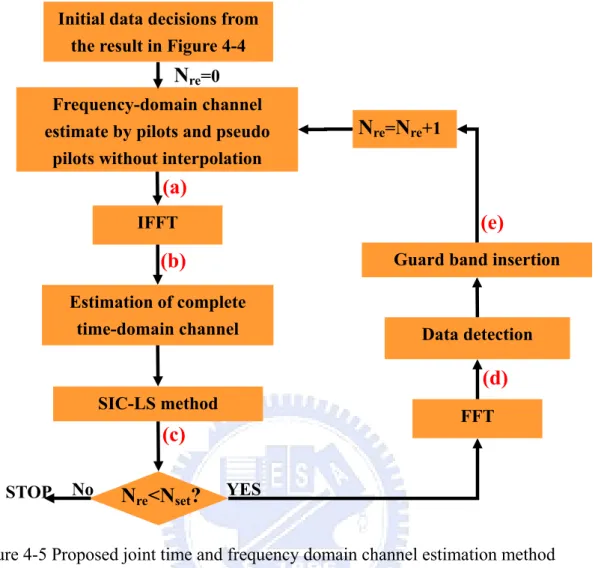
The proposed method uses only one OFDM symbol to conduct the channel estimation. As known, the pilot density is low in DVB-T systems. Direct estimation will result in poor performance. Our idea is to use decisions as pseudo pilots, which will be referred to as pseudo pilots in the sequel, such that the pilot density can be effectively enhanced. The proposed algorithm can be summarized as follows.

1. Obtain an initial channel estimate with one OFDM symbol. 2. Use the estimate with the LS algorithm to conduct data detection.

3. Use some detected data as pseudo pilots and conduct channel re-estimation. 4. Use the re-estimated channel with the LS algorithm to conduct data re-detection. In the following subsection, we will describe each step in details.

4.1 Initial channel estimation with one OFDM symbol

As discussed in Chapter 3, we also conduct an initial frequency-domain channel estimate by pilot information and transfer it to time domain. However, we do not conduct interpolation. Since the pilot density is low, the initial estimate is not accurate. As known, the pilot subcarriers are uniformly spread in the frequency domain. If we only estimate the channel response with those in pilot subcarriers, it is equivalent to conduct a sampling on the frequency-domain channel response. As a result, the time-domain channel response will be periodic.

As known, sampling a frequency domain signal makes its time-domain signal periodic. If the sampling rate is not high enough, aliasing will occur. Figure 4-1 shows the aliasing problem of the channel estimation.

Figure 4-1 Aliasing in initial channel estimation

Let the sampling period be K. It is simple to see that the period of the time- domain channel estimate, denoted withD , will be N/K. In our case, K=12. Consider the 2K mode, ₁ we have N=2048. Thus, we know that the period of the time-domain channel estimate is

about 171 (2048 170.67 171

12 ≅ ≅ ). Let the maximum delay spread of the channel be D . 2

Magnitude

D

1

D

2

t

……

D

1

is

the end of first period

D

2

is

the maximum delay of channel tap