整體式結合迴圈與資料轉換以提升陣列資料區域性

全文

(1)國立交通大學資訊工程系碩士論文. 整體式結合迴圈與資料轉換以提升陣列資料區域性. Improving Array Data Locality by Global Integrated Approach of Loop and Data Transformations. 研究生：沈岳霆指導教授：單智君博士. 中華民國九十三年七月.

(2) 整體式結合迴圈與資料轉換以提升陣列資料區域性. Improving Array Data Locality by Global Integrated Approach of Loop and Data Transformations 研究生：沈岳霆. Student：Yueh-Ting Shen. 指導教授：單智君博士. Advisor：Dr. Jean, Jyh-Juin Shann. 國立交通大學資訊工程學系碩士論文 A Thesis Submitted to Department of Computer Science and Information Engineering College of Electrical Engineering and Computer Science National Chiao Tung University in Partial Fulfillment of the Requirements for the Degree of Master in Computer Science and Information Engineering July 2004 Hsinchu, Taiwan, Republic of China. 中華民國九十三年七月 II.

(3) 整體式結合迴圈與資料轉換以提升陣列資料區域性. 學生：沈岳霆. 指導教授：單智君博士. 國立交通大學資訊工程學系碩士班. 摘要今日高效能的電腦都大量的採用多層記憶體階層的概念。在這些機器上，存取相鄰的記憶體位置將比存取距離較遠的記憶體位置來的快速。因此鼓勵設計者去改變程式記憶體參考的樣式來增加存取相鄰記憶體位置的機會。人工來重新排列程式碼需要清楚的了解機器的架構，是緩慢而且容易出錯的工作，同時也減少了程式的可移植性。因此，使用編譯器來幫助重新排列程式碼是非常值得研究的課題，特別是針對那些有規則資料存取的程式。在這篇論文裡，我們提出了一個整體式結合迴圈與資料轉換的方法來提升資料區域性，基於一個新的區域性模型與簡單的線性代數的技巧。我們提出的區域性模型使用記憶體參考的距離來作量化區域性的標準。對於迴圈內陣列特性我們以跨距向量來表示。然後一個成本的函數就可以從跨距向量導出，以評估程式內不同的陣列參考特性。模擬的結果顯示我們提出來的方法比純粹迴圈或純粹資料的方法有改善。而且這個整體式的考量也比過去的區域考量來的有進步。. i.

(4) Improving Array Data Locality by Global Integrated Approach of Loop and Data Transformations Student：Yueh-Ting Shen. Advisor：Jean, J.J Shann. Institute of Computer Science and Information Engineering National Chiao-Tung University. Abstract High performance computers of today extensively use multiple levels of memory hierarchies. On these machines, the references to a nearby memory location are faster than to a farther location, encourages programmers to modify the references pattern of a program so that the majority of references are made to the nearby memory location. Manual restructuring requires a clear understanding of the impact of the machine architecture, is tedious and error-prone, and results in severely reduced portability. Therefore, compiler optimizations aimed at restructuring code have been very attractive, particularly for programs that exhibit regular data access patterns. In this thesis, we propose a global integrated approach of loop and data transformation to improve data locality, based on a new locality model and simple linear algebra techniques. Our proposed locality model uses reference distance as a metric of the quantity of data locality. To representing data locality characteristics in a loop nest, we use the concept of a stride vector. Then a cost function derived from a stride vector is presented to quantify different occurrences of array references. Simulation results shows our integrated approach does make a difference, and improves over techniques based on pure loop or pure data transformations. Moreover, the proposed global consideration improves over previous pure local consideration. ii.

(5) 誌謝首先要感謝我的指導教授單智君教授，在他辛勤的指導之下，本篇論文得以順利誕生。同時也要感謝他在我研究所這兩年來的教導與勉勵，讓我在知識的學習上有所精進。. 在此也要感謝實驗室的另一位大家長，也是我的口試委員的鐘崇斌教授，以及口試委員謝萬雲博士，由於他們的指教與建議，才使得這篇論文可以更佳的完整與確實。. 感謝陪伴我走過這段時間的每一個人，包括我的家人、朋友、實驗室裡一起努力的同學們。有了你們，讓我在研究的路上走的更順利，進而能更無後顧之憂的從容學習，使我能堅持追求自己的理想。. 所有支持我、勉勵我的師長與親友，所有幫助過我的人，奉上我最誠摯的感謝與祝福，謝謝你們。. 沈岳霆 2004.08.18. iii.

(6) Table of Contents 摘要 ...................................................................................................... i Abstract ................................................................................................ ii 誌謝 .................................................................................................... iii Table of Contents ................................................................................ iv List of Figures..................................................................................... vi List of Tables...................................................................................... vii Chapter 1. Introduction .....................................................................1. 1.1. Locality of Reference.........................................................................2. 1.2. Motivation..........................................................................................3. 1.3. Objective ............................................................................................4. 1.4. Organization of This Thesis ...............................................................4. Chapter 2 2.1. 2.2. 2.3. Background .....................................................................5 The Transformation Fundamentals ....................................................5. 2.1.1. Linear Algebra Representation of Array References ..................5. 2.1.2. Unimodular Transformation .......................................................6. Loop Transformation .........................................................................8 2.2.1. Loop Interchange ......................................................................10. 2.2.2. Loop Reversal ...........................................................................10. 2.2.3. Loop Skewing ........................................................................... 11. Data Transformation ........................................................................12 2.3.1. Unimodular Data Transformations ...........................................12. 2.3.2. Hyperplane Concepts................................................................14. 2.4. Integrated Approach of Loop and Data Transformations ................15. 2.5. Related Work....................................................................................16 iv.

(7) 2.5.1. Exhaustive Search Approach ....................................................16. 2.5.2. Heuristic Approach ...................................................................17. 2.6. Summary and Comparison...............................................................18. Chapter 3 3.1. Proposed Global Integrated Approach ..........................20 Problem Description ........................................................................20. 3.1.1. Array Reference Representation...............................................20. 3.1.2. Temporal locality ......................................................................21. 3.1.3. Spatial locality ..........................................................................21. 3.1.4. Integrated Approach..................................................................22. 3.2. Locality Estimation Model ..............................................................23 3.2.1. Reference Distance ...................................................................24. 3.2.2. Stride Vector..............................................................................24. 3.3. Framework of Proposed Approach ..................................................26. 3.4. Three Steps of Proposed Approach..................................................27 3.4.1. Local Loop and Data Transformation Selection .......................27. 3.4.2. Global Data Transformation Decision ......................................29. 3.4.3. Local Loop Transformation Refinement...................................30. Chapter 4. Simulation and Analysis................................................31. 4.1. Simulation Environment ..................................................................31. 4.2. Simulation Results and Analysis......................................................36 4.2.1. Execution Times .......................................................................37. 4.2.2. Cache Miss Rate .......................................................................38. 4.2.3. Simulation Analysis ..................................................................40. Chapter 5. Conclusion and Future Works .......................................42. References...........................................................................................44. v.

(8) List of Figures. Figure 2-1 An example of the array reference representation........................................6 Figure 2-2 Examples of three types of the unimodular matrix ......................................7 Figure 2-3 Examples of 2D space using unimodular transformations...........................8 Figure 2-4 An example of loop interchange ................................................................10 Figure 2-5 An example of loop reversal ...................................................................... 11 Figure 2-6 An example of loop skewing...................................................................... 11 Figure 2-7 Examples of unimodular data transformation ............................................13 Figure 3-1 The framework of proposed approach .......................................................27 Figure 4-1 Compilation flow of proposed approach....................................................32 Figure 4-2 Execution time with varying problem size.................................................37 Figure 4-3 Speedup for the different version of transformations ................................38 Figure 4-4 Memory reference percentage of different memory hierarchies................39 Figure 4-5 Cache miss ratio for L1 and L2 cache........................................................40. vi.

(9) List of Tables. Table 2-1 Array layouts of 2-dimensional array and associated hyperplanes..............15 Table 2-2 Summary of loop and data transformations.................................................16 Table 2-3 Comparison between related works.............................................................19 Table 4-1 Platform used in the experiments to measure execution time .....................33 Table 4-2 Platform used in the experiments to simulate cache behavior.....................35 Table 4-3 Benchmark programs used in the simulation...............................................36 Table 4-4 Different transformed version used in the simulation .................................36. vii.

(10) Chapter 1. Introduction. High performance computers of today extensively use multiple levels of memory hierarchies. On these machines, references to a nearby memory location are usually faster than references to a farther location. This renders the performance of applications critically dependent on their memory access characteristics and encourages programmers to modify the references pattern of a program so that the majority of references are made to a nearby memory location. In particular, careful choice of memory-sensitive data layouts and code restructuring appear to be crucial. Unfortunately, the lack of automatic tools forces many programmers need to restructure their code manually. The problem is exacerbated by the increasing sophisticated nature of applications. Manual restructuring requires a clear understanding of the machine architecture, is tedious and error-prone, and results in severely reduced portability. Therefore, compiler optimizations aimed at restructuring code have been very attractive, particularly for programs that exhibit regular data access patterns. In this thesis, we propose a global integrated approach of loop and data transformations to improve data locality. The type of data transformations includes changing memory layouts such as row-major or column major storage of multi-dimensional arrays (which are common data structures in regular applications). In this chapter, we briefly introduce the locality property of reference, basic compiler transformation techniques to improve data locality, and the motivation and objective of this thesis.. 1.

(11) 1.1 Locality of Reference Over the last decade, the speed gap between processor and memory access has continued to widen. Computer architects have tuned increasing to the use of memory hierarchies with one or more levels of memory. Almost all general-purpose computer systems, from personal computers to workstations of large systems, have a memory hierarchy comprising different speed of memory levels. Main memory latencies for new machines are now more than hundred cycles. This has resulted in the increasing reliance on caches as a means to increase the overall memory bandwidth and reduce memory latency. These small, fast memories are only effective when programs exploit locality. Data locality is the property that references to the same memory location and nearby locations are reused within a short period of time. There are two types of locality—temporal locality and spatial locality. Temporal locality occurs when two reference refer to the same memory location. Spatial locality occurs when two references refer to nearby memory locations. Manual restructuring programs in order to improve locality requires a clear understanding of the detail of the machine architecture, which is a tedious and error-prone task. Instead, achieving good data locality should be the responsibility of the compiler. By placing the burden to the compiler, programs will be more portable because programmers will be able to achieve good performance without making machine-dependent source-level transformations. Previous research in compiler generally concentrated on iteration space transformations to improve locality. Among these techniques used are unimodular and non-unimodular iteration space transformations, tiling, and loop fusion. All these techniques focus on improving data locality indirectly as a result of modifying the iteration space traversal order. 2.

(12) Recently, data transformations have been proposed to improve data locality because loop transformations are not always effective. Instead of changing the order of loop iterations, data transformations modify the memory layouts of multi-dimensional arrays (form a language-defined default such as column-major in FORTRAN and row-major in C into a desired form).. 1.2 Motivation Compiler researchers have developed loop transformations that allow the conversion of programs to exploit locality. Recently, transformations that change the memory layouts of multi-dimensional arrays—called data transformations—have been proposed. While loop transformations can improve data locality, are well-understood and effective in many cases, they have at least three important drawbacks: (1) they are constrained by data dependencies; (2) complex imperfectly nested loops pose a challenge for loop transformations; and (3) they affect the locality characteristics of all the data sets accessed in a nest, some perhaps adversely. Nevertheless, data transformations have some disadvantages. Constructs such as pointer arithmetic in C and common blocks in FORTRAN may prevent memory layout transformations by exposing unmodifiable layouts to the compiler. A key draw back is that data transformations do not improve temporal locality. As mentioned above, neither loop nor data transformations are fully effective in optimizing locality. For our observation, previous research about integrated loop and data transformations did not concern the correlation between different loops and between different types of transformations. This means that benefits for a single loop nest may sacrifice benefits for another loop nest. If we can consider the effect of different transformations globally, we may improve the data locality compared with 3.

(13) previous research.. 1.3 Objective Many scientific programs and image processing applications operate on large multi-dimensional arrays using multi-level nested loops. Both changing the execution order and the data layout will affect data locality. The loop transformations involve changing the execution order of loop iterations. The data transformations involve changing the array layouts in memory. Our objective is to find a global integrated approach of loop and data transformations to improve array data locality for all loops in a whole program.. 1.4 Organization of This Thesis This thesis is organized as follows. Chapter 2 introduces the background of compiler transformations and discusses previous related work on improving data locality. In Chapter 3, we describe our global integrated approach in detail. Then the simulation environment and simulation results are presented in chapter 4. Finally, we summarized our conclusions and future works in Chapter 5.. 4.

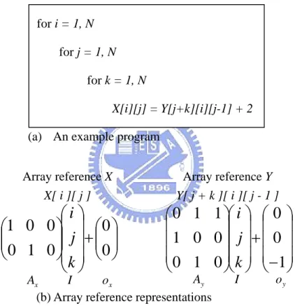
(14) Chapter 2. Background. In this chapter, we first introduce the linear algebra representation of array references in the loop nests. This representation and linear algebra techniques simplify the transformation works. Then the fundamentals of loop transformations and data transformations are described. The following sections present related works about the integrated approach of loop and data transformations. Finally, we give a comparison between loop transformations and data transformations and summarize previous researches.. 2.1 The Transformation Fundamentals The main transformation method of previous research is based on linear algebra techniques [9]. In this section we describe linear algebra representation of array references and transformation matrices.. 2.1.1 Linear Algebra Representation of Array References Consider an array reference to an m -dimensional array in a loop nest of depth n . We assume that the array subscript functions and loop bounds are affine functions. of enclosing loop indices and symbolic variables, which affine functions are the linear combination of the index variables plus a constant. Let I denotes the iteration vector consisting of loop indices starting from the outermost loop to the innermost loop; each array reference can be represented by AI + o. where the m × n matrix A is called the array reference matrix and the 5.

(15) m -element vector o is called the array offset vector. Note that each row of A. corresponds to a dimension of the array; and each column of A gives information of array references about the corresponding loop index. In particular, the locality behavior of the innermost loop is determined by the last column of A . Here we give a program in Figure 2-1 (a) as an example and describe the representation of array references in Figure 2-1 (b).. for i = 1, N for j = 1, N for k = 1, N X[i][j] = Y[j+k][i][j-1] + 2 (a) An example program Array reference X X[ i ][ j ]. Array reference Y Y[ j + k ][ i ][ j - 1 ]. ⎛i⎞ 1 0 0 ⎞⎜ ⎟ ⎛ 0⎞ ⎛ ⎟⎟⎜ j ⎟ + ⎜⎜ ⎟⎟ ⎜⎜ 0 1 0 ⎠⎜ k ⎟ ⎝ 0⎠ ⎝ ⎝ ⎠. ⎛ 0 1 1⎞⎛ i ⎞ ⎛ 0 ⎞ ⎜ ⎟⎜ ⎟ ⎜ ⎟ 1 0 0 ⎜ ⎟⎜ j ⎟ + ⎜ 0 ⎟ ⎜ 0 1 0⎟⎜ k ⎟ ⎜ −1⎟ ⎝ ⎠⎝ ⎠ ⎝ ⎠. Ay Ax I ox (b) Array reference representations. I. oy. Figure 2-1 An example of the array reference representation. 2.1.2 Unimodular Transformation If we describe array references in a program as matrices in linear algebra, then the transformations applied on a program can be represented as matrices in linear algebra, too. Each transformation matrix corresponds to a transformation method. The transformation method such as interchanging, reversal and skewing can all be unified 6.

(16) by casting them as the linear transformation method. Such a framework allows a compiler to perform several transformations in one step. In other words, if we want to do more than one transformation at the same time, it is only need to do one combination transformation, which is composed of all transformations we want to do. Composition of linear transformations is performed by multiplying the transformation matrices. These kinds of transformation matrices are all unimodular matrices [11]. We give an example of the transformation matrix of unimodular transformations as Figure 2-2 shows.. ⎛ 0 1 0⎞ ⎟ ⎜ ⎜ 0 0 1⎟ ⎜ 1 0 0⎟ ⎠ ⎝. ⎛1 ⎜ ⎜0 ⎜0 ⎝. (a) Interchange. 0 −1 0. (b) Reversal. 0⎞ ⎟ 0⎟ 1 ⎟⎠. ⎛1 0 ⎜ ⎜0 1 ⎜3 0 ⎝. 0⎞ ⎟ 0⎟ 1 ⎟⎠. (c) Skewing. Figure 2-2 Examples of three types of the unimodular matrix. All these three types of transformations are unimodular; that is, the transformation matrices are unimodular. The definition of unimodular transformation matrix is the absolute value of the determinant of a transformation matrix is 1. There are several characteristics of unimodular transformation matrices: (1) The transformations matrix is a square matrix which maps an n -dimensional space to another n -dimensional space. (2) The transformation matrix has all integral components, so it maps an integer point to another integer point. (3) The product of two unimodular matrices is unimodular.. 7.

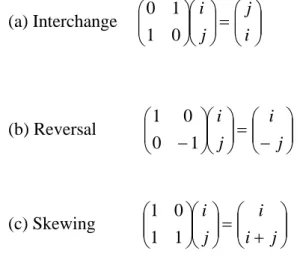
(17) (4) The inverse of an unimodular matrix is unimodular.. (a) Interchange. ⎛ 0 1 ⎞⎛ i ⎞ ⎛ j ⎞ ⎟⎟⎜⎜ ⎟⎟ = ⎜⎜ ⎟⎟ ⎜⎜ ⎝ 1 0 ⎠⎝ j ⎠ ⎝ i ⎠. (b) Reversal. ⎛ 1 0 ⎞⎛ i ⎞ ⎛ i ⎞ ⎟⎟⎜⎜ ⎟⎟ = ⎜⎜ ⎟⎟ ⎜⎜ ⎝ 0 − 1⎠ ⎝ j ⎠ ⎝ − j ⎠. (c) Skewing. ⎛ 1 0 ⎞⎛ i ⎞ ⎛ i ⎟⎟⎜⎜ ⎟⎟ = ⎜⎜ ⎜⎜ ⎝ 1 1 ⎠⎝ j ⎠ ⎝ i +. ⎞ ⎟ j ⎟⎠. Figure 2-3 Examples of 2D space using unimodular transformations. The unimodular transformation means that the integer points of the original iteration space will be mapped onto integer points in the transformed space (because the transformation matrix has integer entries), and the volume of the iteration space is preserved (because the determinant of the transformation is ± 1 ). For a dense iteration space, such as a normalized index set, every integer point in the image space corresponds to an integer point in the original iteration space. In other words, if the original iteration space is dense, so is the transformed space. The 2-dimensional space transformations using unimodular transformations are showed in Figure 2-3.. 2.2 Loop Transformation When optimizing the performance of programs, the most gains will come from optimizing the region of the program that requires the most time—the repetitive region of the program. These correspond either to iterative loop or recursive procedures. Here we concentrate on optimizing loops. For the most part we will focus 8.

(18) on countable loops, where the trip counts can be determined without executing the loop, as opposed to while loops. Most presentations of loop restructuring methods focus on the legality and benefits of performing a transformation or optimization. The benefits of a transformation cannot be determined until the target computer architecture is known. Likewise, the legality of a transformation depends on the semantics of the target machine and language. Most machines today comprise one or more sequential processors connected in some fashion, so we will concentrate on compiling for collections of sequential machines. The transformation is legal if it preserves the dependence relations. For sequential loops, this means that the dependence distance vector must still be lexicographically nonnegative. The characteristics of the unimodular matrices explain why we use it as the category of our transformations. There are two advantages of unimodular loop transformations. First, combinations of multiple transformations can be represents as products of the elementary unimodular transformation matrices, so a compound transformation is simplified. Second, the legality test of loop transformations is simplified to matrix operations, so we can easily examine which transformation is legal or not. Let a loop transformation be represented by a square non-singular integer matrix TL . Assuming that I is the original iteration vector and I ' = TL I is the new −1. iteration vector; each occurrence of I in the loop body is replaced by TL I ' . So. each reference represented by AI + o is transformed to −1. ATL I '+o Loop transformations for locality are relatively well studied; we will only describe the fundamental principle here, for in-depth discussion of several approaches 9.

(19) can be found in [1][12][13].. 2.2.1 Loop Interchange Perhaps the single most important loop restructuring transformation is the loop interchange. Interchanging two tightly nested loops switches the inner and outer loop; it was developed initially to help with automatic discovery of parallelism. Converting a sequential nested loop into parallel form would try to find a loop that carried no dependence relations. If one loop carried all the dependence relations, that loop would be interchanged to the outermost position, and the rest of the loops would be executed in parallel. The transformation matrix of interchanging we give an example as Figure 2-4. for i = 0,N. ⎛ 0 1⎞ ⎜⎜ ⎟⎟ 1 0 ⎝ ⎠. for j = 0,N U[ i ][ j ] (a) Original program. (b) Transformation matrix. for j = 0,N for i = 0,N U[ i ][ j ] (c) Transformed program. Figure 2-4 An example of loop interchange. 2.2.2 Loop Reversal The compiler can decide to run a loop backward; this is called loop reversal. If a sequential loop carries a dependence relation, revering the loop will reverse the direction of the dependence, violating that dependence relation. Thus, loop reversal is legal only when the loop carries no dependence relations. The transformation matrix of reversal we give an example as Figure 2-5.. 10.

(20) for i = 0,N for j = 0,N. ⎛1 0 ⎞ ⎜⎜ ⎟⎟ 0 −1 ⎝ ⎠. for i = 0,N for j = 0,-N. U[ i ][ j ] (a) Original program. U[ i ][ j ] (b) Transformation matrix. (c) Transformed program. Figure 2-5 An example of loop reversal. 2.2.3 Loop Skewing The normalization can change the shape of the iteration space. Because the shape of the iteration space changes, as does the dependence distances. It can affect the ability to interchange loops. If normalization can prevent interchanging, then perhaps unnormalization can enable interchanging. We call this loop skewing. Loop skewing changes the iteration vectors for each iteration by adding the outer loop index value to the inner loop index. Choosing whether to skew and the factor by which to skew is driven by the goal to enable other transformations or to improve parallelism after another interchanging. The transformation matrix of skewing we give an example as Figure 2-2 (c). for i = 0,N for j = 0,N U[ i ][ j ] (a) Original program. ⎛1 0 ⎞ ⎜⎜ ⎟⎟ 1 1 ⎝ ⎠ (b) Transformation matrix. for i = 0,N for j = i,i+N U[ i ][ j ] (c) Transformed program. Figure 2-6 An example of loop skewing. 11.

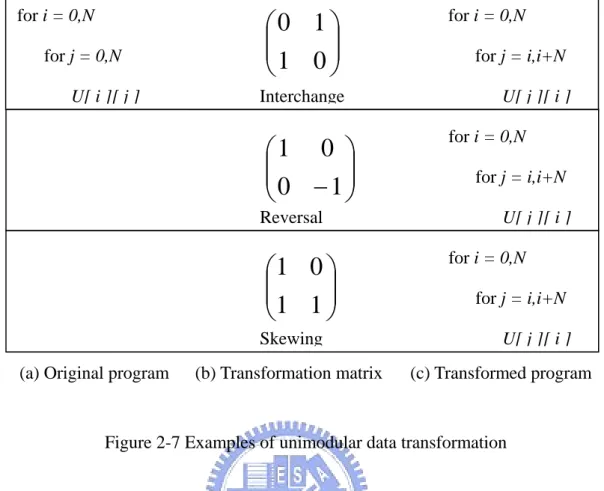
(21) 2.3 Data Transformation Data transformation [8][10] is another approach. Array is a general data structure and often seen in most programs because it is a simple and intuitional representation of data. Therefore, many scientific programs and image processing applications operate on large multi-dimensional arrays using multi-level nested loops. The meaning of data in this thesis is equally to array structure. In the following we use the term “data” and “array” alternately. Conceptually, a data transformation is applied by transforming array subscripts of the array reference . Let a data transformation be represented by s square non-singular integer matrix TD . Then each reference represented by AI + o is transformed to TD AI + TD o. Notice that in contrast to loop transformations, the iteration vector does not change but offset vector is transformed.. 2.3.1 Unimodular Data Transformations The data transformations we consider are as same as the loop transformations described in section 2.2. We only consider unimodular transformations including interchange, reversal and skewing. A similar example which the transformation matrix is as same as loop transformation but adopted by data transformation is showed in Figure 2-7. There are two advantages of unimodular data transformations. First, the array index computation is efficient because in unimodular transformations the variable must involve only integers. Second, the transformed data space is equal to the original one, so the memory usage is efficient.. 12.

(22) for i = 0,N for j = 0,N U[ i ][ j ]. ⎛ 0 1⎞ ⎜⎜ ⎟⎟ 1 0 ⎝ ⎠. for i = 0,N for j = i,i+N. Interchange. U[ j ][ i ] for i = 0,N. ⎛1 0 ⎞ ⎜⎜ ⎟⎟ 0 −1 ⎝ ⎠. for j = i,i+N U[ j ][ i ]. Reversal. for i = 0,N. ⎛1 0 ⎞ ⎜⎜ ⎟⎟ 1 1 ⎝ ⎠. for j = i,i+N U[ j ][ i ]. Skewing (a) Original program. (b) Transformation matrix. (c) Transformed program. Figure 2-7 Examples of unimodular data transformation. We can divide the problem of optimizing array layouts into two independent sub-problems. First, determining optimal array layouts; and second, determining data transformation matrices to implement optimal array layouts. Each sub-problem can be solved independently. Previous research offered algorithms to handle the first sub-problem where as a few offered methods to handle the second problem. In fact, the second problem arises because there is no way of specifying the array layouts in conventional languages like FORTRAN and C. The main data transformation objective of this thesis is to find the optimal array layouts for all array references in the whole program. Once we decide a suitable array layout for each array, it is a mechanical process to find the corresponding data transformation matrices to implement the chosen layouts. This is the reason to make our approach easy to adapt to languages with different default layouts as well as to. 13.

(23) have explicit memory layout representations. Next we will describe our representation of array layouts, called hyperplane.. 2.3.2 Hyperplane Concepts We use the hyperplane concepts [6] to represents the layout of an array. In an m-dimensional space, a hyperplane can be defined as a set of tuples (a1 , a 2 ,..., a m ) such that g1a1 + g 2 a 2 + ... + g m a m = c , where g1 , g 2 ,..., g m are rational numbers called hyperplane coefficients and c is a rational number called hyperplane constant. A hyperplane vector (g1 , g 2 ,..., g m ) defines a hyperplane family where each member hyperplane has the same hyperplane vector but a different c value. For convenience, we use a row vector g T = (g1 , g 2 ,..., g m ) to denote such a hyperplane family whereas g corresponds to the column vector representation of the same hyperplane family.. We say that two data points (array elements). d1. and. d2. (in a. multi-dimensional array) belong to the same data hyperplane g if g T d1 = g T d 2. Two data points d 1 and d 2 are said to have spatial locality for a given data hyperplane g T if above equation holds for them. For example, in a two-dimensional array space, a hyperplane vector such as (0,1) indicates that two array elements belong to the same hyperplane as long as they have the same value for the column index; the value of the row index does not matter. Two data elements may belong to more than one hyperplane as well. For example, in a three-dimensional array space, two data elements may belong to a hyperplane. (0,0,1). as well as to another hyperplane (0,1,0) . A few possible array layouts and. their associated hyperplane vectors for two-dimensional case are given in Table 2-1.. 14.

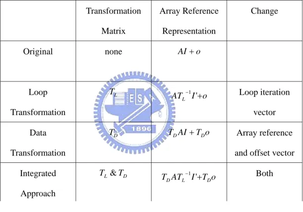
(24) Table 2-1 Array layouts of 2-dimensional array and associated hyperplanes row-major. column-major. Diagonal. anti-diagonal. (1,0). (0,1). (1,-1). (1,1). 2.4 Integrated Approach of Loop and Data Transformations The loop and data transformation is different in many ways. The comparison is presented as follows. Loop transformation:. (1). Constrained by data dependences. (2). Difficulty applicable to complex imperfect nested loops. (3). The effect is local, only affects the loop nest to which it is applied. (4). Improve temporal and spatial locality. Data transformation:. (1). Not constrained by data dependences. (2). Easily applicable to perfect and imperfect nested loops. (3). The effect is global, affects every part of the program that access the array. (4). Improve spatial locality. These two approaches are not conflicting, so the combination of loop and data transformations is an attractive approach. But determining both loop and data transformation matrices are a non-linear problem. We now show that for a single reference, determining both a loop and a data transformation matrix simultaneously is equivalent to solving a non-linear system with some additional constraints in Table 2-2. Suppose that the original reference is AI + o , and we would like to apply a loop transformation matrix TL and a data transformation matrix TD . Then the −1. transformation reference is TD ATL I '+TD o . Omitting the offset vector part [4], since 15.

(25) both TD and TL. −1. are unknown, determining a suitable TD LTL. −1. from the locality. point of view involves solving a non-linear problem, with the additional constraints such that both TD and TL should be non-singular and TL should observe all the data dependences in the original loop nest.. Table 2-2 Summary of loop and data transformations. Transformation. Array Reference. Matrix. Representation. Original. none. AI + o. Loop. TL. ATL I '+o. −1. Transformation Data. Loop iteration vector. TD AI + TD o. TD. Array reference and offset vector. Transformation Integrated. Change. TL & TD. −1. TD ATL I '+TD o. Both. Approach. 2.5 Related Work In this section we will introduce several previous research topics related to the integrated approach, including an exhaustive search approach and a heuristic approach.. 2.5.1 Exhaustive Search Approach This previous work [3] presents a unified approach to locality optimization that 16.

(26) employs both data and loop transformations. The compiler optimizations are based on an algebraic representation of data mappings, and a new data locality model. They consider computers with large main memory and smaller, but faster cache memory. Cache hit ratio is one metric for quantifying data locality, but the hit ratio for a given run of a program is a non-trivial function of machine parameters, operating system policies, load on the machine and the access pattern of the program itself. A more machine-independent metric, which can be used in compilers, is reference distance. They use reference distance as a metric of the quality of data locality. This metric is not as accurate for a given machine as the locality hit ratio, but it has the advantage of being relatively independent from machine parameters. Reference distance for a given memory access is defined to be the number of distinct cache lines accessed since the last access to the same cache line (or 0 if the cache line has not been accessed before). The goal of the locality optimization is to decrease the distances for critical references. Note that to decrease the distance for some reference may lead to increase the distance for others. Their approach to representing data locality for different data mappings uses a new concept of stride vector instead of the more traditional reuse vectors. Elements of the stride vector give us information about data locality. If an element is 0, then this loop carries temporal locality, if an element is less than the size of a cache line, then the loop has spatial locality. So their solution is to find the transformation matrix and array layout vector to satisfy TL v = Am . The desired reference vector is presented by v and the array layout vector is presented by m .. 2.5.2 Heuristic Approach This paper [5] describes an integrated compiler approach to enhance cache locality. Their approach combines loop and data transformations, but specializes the 17.

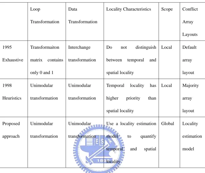
(27) loop transformations for optimizing temporal locality. Once the potential temporal locality is exploited, their approach uses data transformations to optimize available spatial reuse in the loop nest. This technique can be extended to work with cases in which some subset of the arrays referenced in the loop nest had fixed memory layouts. Multiple loop nests. When there are many loop nests in a program, their approach is rather simple. They need to determine an order of processing the nests, if a nest is more important (costly) than another one, they optimize the more important nest first. Profiling can be used to determine the estimated cost of a loop nest. After optimizing this nest, it is possible that the memory layouts of some of the arrays referenced will be fixed. Then, they consider the next important nest and optimize it. Take all the layouts determined so far into account, and so on. Conflict-free layouts solution. If the references to the same array in a loop nest span more than one uniformly generated set, then a conflict resolution scheme as discussed in the previous hyperplane based approach can be used.. 2.6 Summary and Comparison This section we summarize the difference between loop and data transformations and previous research. Loop transformations involve changing the execution order of programs but data transformations involve changing the array layout in memory. The comparison of related work is described in Table 2-3.. 18.

(28) Table 2-3 Comparison between related works Loop. Data. Transformation. Transformation. Locality Characteristics. Scope. Conflict Array Layouts. 1995. Transformaiton. Interchange. Do. Exhaustive. matrix. transformation. between. contains. not. distinguish temporal. Local. array. and. layout. spatial locality. only 0 and 1 1998. Unimodular. Unimodular. Temporal. Heuristics. transformation. transformation. higher. locality priority. has. Local. layout. Proposed. Unimodular. Unimodular. Use a locality estimation. approach. transformation. transformation. model temporal locality. 19. and. Majority array. than. spatial locality. to. Default. quantify spatial. Global. Locality estimation model.

(29) Chapter 3. Proposed Global Integrated Approach. In this chapter, we present our global integrated approach to enhance array data locality for whole program. There are four sections in this chapter. The first one is problem description, which describes the problem formulation and the difficulty. The second part is the basic concept of locality estimation model, including reference distance and stride vector. The third one describes the framework of proposed integrated approach. Finally, we showed three steps in the framework in detail.. 3.1 Problem Description The global consideration problem is to decide the array layout which exploits most data locality in the whole program. The preferred array layout in the local consideration may not identical between different loop nests.. 3.1.1 Array Reference Representation Consider an array reference to an m -dimensional array in a loop nest of depth n . We assume the array subscript functions and loop bounds are affine functions of. enclosing loop indices and symbolic variables. Our approach uses the same presentation from previous research discussed in Chap 2. An array reference can be represented by AI + o. where I denotes the iteration vector (consisting of loop indices starting form the outermost loop), the m × n matrix A denotes the reference matrix of an array reference and the m -element vector o denotes an array offset vector. As offset 20.

(30) vectors are irrelevant from the locality analysis point of view, for simplify, the constant part is ignored.. 3.1.2 Temporal locality We treat the property of temporal locality as the natural characteristics of the program, in other words, it never changes no matter what data transformations applied. An array reference in a loop nest could exploit temporal locality if and only if ∅ ∉ ker{A}. Let a1 ,..., a n denote the first to the last column of inverse of the loop transformation matrix, respectively. The innermost loop exhibits temporal locality with respect to a reference if. an ∈ ker{A} The outermost loop exhibits temporal locality with respect to a reference R if a1 ∈ ker{A}. 3.1.3 Spatial locality We view the iteration space of a loop nest of depth n as an n -dimensional space where each point is denoted by an n × 1 column vector. Let is now concentrate on two consecutive iterations I and I next of a given loop nest of depth n . Such two iterations have identical values for each loop index except for the innermost loop, i.e., I = (i1 ... in −1 in ). T. and I next = (i1 ... in −1 in + 1) . In order to exploit the T. locality for reference denoted by a reference matrix A , two consecutive iterations I and I next defined above should reference two data elements that have spatial locality in the data space. In particular, we want the distance of referenced elements is as close as possible so that the possibilities they can reside on the same (or at least neighboring) 21.

(31) block of the same memory level increased. We use the hyperplane concept to represent array layouts. The innermost loop exhibits spatial locality with respect to a reference (denoted by an m × n reference matrix A ) to an m -dimensional array, if, for each hyperplane vector g defining the memory layout,. g ∈ ker{a m } where a m is the row vector form of the last column of A . The outermost loop exhibits spatial locality with respect to a reference to an m -dimensional array for each hyperplane vector g defining the memory layout, g ∈ ker{a1 }. where a1 is the row vector form of the first column of A .. 3.1.4 Integrated Approach As previous related work results show, data transformations can only affect spatial locality. A key drawback is that data transformations do not improve temporal locality. Although loop transformations can affect both temporal and spatial locality, but loop transformations mainly focus on temporal locality. The effect of loop transformations on spatial locality is based on the default array data layout, i.e., FORTRAN is column major, C is row major. Our framework first optimized the temporal locality in a loop nest for most number of references. It then focuses on exploiting spatial locality for all references (including references which have temporal locality) in a loop nest. We pay more attention to inner loop than to outer loop. Given the fact that the innermost loop is concerned obtaining temporal locality is more important (and better) than obtaining just spatial locality, we have improvement over the original programs. After each loop nest is analyzed, we can select a local array layout is most 22.

(32) suitable for the array reference in a loop nest. For a global data array, if array layouts selected in all loop nests are all the same, then the solution of global array layout is trivial. But if array layouts selected in different loop nests are different, then the conflict situation occurs, we use a cost function to decide which layout is better for array data locality. We divide the problem of improving locality by data transformations into two independent sub-problems: (1). Determination of the optimal array data layouts that are defined by hyperplanes. (2). Data space transformation matrices to obtain (or implement) the optimal layouts. Our research mainly focuses on the first problem, finding global array layouts for improving data locality. An integrated approach of loop and data transformations has great effect on the locality analysis.. 3.2 Locality Estimation Model We want to optimize programs for execution time. To exploit the memory hierarchy, data locality has to be maximized. To simplify our discussion, we only consider computers with large main memory and smaller, but faster cache memory. Cache hit ratio is one metric for quantifying data locality. The hit ratio for a given run of a program is a non-trivial function of machine parameters, operating system policies, load on the machine and the access pattern of the program itself. A more machine-independent metric, which can be used in compilers, is reference distance. We measure how many different data elements are separated between two contiguous data reference. We observe that this reference distance can be 23.

(33) used to guild program transformations. As a locality model, we use the stride vector concept to measure the locality of array references in a loop nest. We will show how reference distance and stride vector concept to quantify different types of locality, between different loop nests and between different array references.. 3.2.1 Reference Distance The reference distance can be used as a metric of the quality of data locality. This metric is not as accurate for a given machine as the cache hit ratio, but it has the advantage of being relatively independent from machine parameters. Reference distance for a given array is defined to be the number of distinct elements between contiguous references to the same array element (or 0 if the array element has not been referenced before). To analyze the program behavior, we examine all memory reference of the array data. Note that to decrease the distance for some references may have to increase the distance for others. The goal of the locality optimization is to decrease the global reference distance for whole program. The definition of reference distance in this thesis is different from previous research. Previous definition of reference distance is how many different data elements are referenced between two references to the same data. The previous concept of reference distance is about the relationship in time domain; however, our proposed scheme is concern about the spatial relationship between memory references.. 3.2.2 Stride Vector Our approach to represent data locality for different array layouts uses a concept 24.

(34) of a stride vector instead of the traditional reuse vectors. Stride vector is defined as array layouts memory reference distance, for a given array layouts, the reference distance between two contiguous memory references. Elements of the stride vector give us information about data locality. If an element is 0, then this loop carries temporal locality, if an element is less than the block size of a memory hierarchy, then the loop has spatial locality. The stride vector of an array reference can be calculated from the reference matrix, the array size of each array dimension, and the hyperplane vector from the array layouts. To simplify our discussion, we only consider the array size of each dimension is equal, that is, a 2-dimensional array is like a square matrix. Let the reference matrix is denoted by an m × n matrix A , the size of each array dimension is all equal by k , the array layout is denoted by vector g , then the stride of an array reference can be compute as. (. MemoryLayoutVector (g ) = k g1 , k g2 ,..., k gm. ). stride(g ) = MemortLayoutVector (g ) • An Let the reference matrix is denoted by A , the vector of the last column of A is denoted by. a m , the hyperplane vector of. (g1 , g 2 ,... g m )T. is denoted by g , the size of each array dimension is denoted by k ,. m -dimensional array layouts. the stride vector of this array reference is denoted by S .. (. S = k g1 , k g 2 ,..., k g m. ). T. The locality of an array reference in a loop nest is estimated by: ArrayLocality ( A, g ) = iterations × stride(g ). So the global locality of an array is the summation of locality in all loop nests, estimated by:. 25.

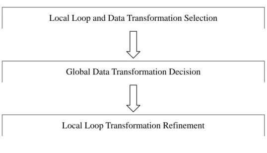
(35) GlobalArrayLocality ( A, g ) =. all. ∑ ArrayLocality ( A, g ) loops. But we need to adjust the quantity score to an inverse ratio so that the higher score means the better locality. This is the nature representation. So the locality estimation function is presented by 1 all. ∑ ArrayLocality( A, g ) loops. 3.3 Framework of Proposed Approach In this section, we describe the framework of proposed global integrated approach of loop and data transformations. First, we will describe our array reference representation which is based on previous research. Next, we will have a brief introduction about how to exploit temporal and spatial locality and what is the global integrated approach. The global integrated approach is further divided into two stages, the first stage is called local transformation selection stage, and the second stage is called global transformation decision stage. In the local stage, we exploit temporal and spatial locality on a single loop nest without considering other loop nests. In the global stage, we examine selections from the first stage and check whether there are conflict array layouts or not. If there are conflict array layouts in the program, we resolve the conflict by a cost function.. 26.

(36) Local Loop and Data Transformation Selection. Global Data Transformation Decision. Local Loop Transformation Refinement. Figure 3-1 The framework of proposed approach. 3.4 Three Steps of Proposed Approach In this section, we present our integrated approach to enhance data locality in a single loop nest. This local loop and data selection stage is used to produce necessary information to guild transformations in the next global data transformation stage, this part only focus on a single loop nest without considering other loop nests. Finally, we need to do a local loop transformation refinement to adapt global inconsistency. For a single reference, determining both a loop and a data transformation matrix simultaneously is equivalent to solving a non-linear system with some additional constraints. As mentioned earlier, our approach is based on optimizing temporal locality using loop transformations and optimizing spatial locality via data transformations.. 3.4.1 Local Loop and Data Transformation Selection We divided this stage into two phases. The first phase uses loop transformation concept to explore temporal locality; the second phase uses data transformation. 27.

(37) concept to explore spatial locality. (1) Temporal locality exploration. Loop transformation can improve both temporal and spatial locality, however, at this phase we only want to explore the potential temporal locality of loop transformations. Our framework first finds the temporal locality in the innermost loop nest for most number of references. Let the reference matrices of array references in the loop nest be L1 , L2 ,..., Lk . Our approach first computes the spanning vectors for the kernel sets of these reference matrices. Consider all references, from among all spanning vectors, we choose the one which occurs most frequently. This approach tends to maximize the number of references for which temporal locality can be exploited. (2) Spatial Locality Exploration. Data transformation can only improve spatial locality, at this phase, we want to explore the potential spatial locality of data transformations. A data transformation matrix we exploited for an array reference implies an associated array layout. Previous research only exploit spatial locality for array references without temporal locality, however, our approach exploit spatial locality for all references no matter they have temporal locality or not. Nevertheless, references without temporal locality have higher priorities over the references with temporal locality. We use hyperplane concept to represent array layouts, that is, for any given array layout, there is an associated hyperplane vector correspond to. To simplify our discussion, we consider in each loop nest there is a hyperplane vector corresponding to one optimal array layout. Our search for potential spatial locality starts at the last nonzero column denotes by a m , from inner loop to outer loop. Because a zero column simply implies the array reference corresponding to the loop nest exhibits temporal locality. 28.

(38) 3.4.2 Global Data Transformation Decision There are many loop nests and data arrays in the whole program, different loop nests maybe reference the same array; different arrays could be referenced in the same loop nest. In the previous related work, they do not consider the conflict situation when the array data layout determined by different loop nest is different. In this section we discuss the main technique how we extend our approach to handle the multiple loop nest case. In the local stage, we have found all potential temporal and spatial locality. However, not all potential locality can exist at the same time. Our proposed method would use a global array layout solution to avoid conflict array layout situation, in other words, we do not consider changing array layouts at run time. Conflict Array Layouts. The problem of determining of the optimal array data layouts has some factor which needs to consider separately. Because the effect of a data transformation is global in the sense that decisions regarding the memory layout of an array influence the locality characteristics of every part of the program that references the array. So we need to consider the following situation: layouts of some of the array references are constrained or fixed. If an array references is fixed, the changing of array data layout of that array is illegal because this transformation cannot guarantee the result is correct. If an array reference in a loop nest is constrained by other loop nest, then we need to decide which array layout will be used. Resolution of Conflict Situation. If the references to the same array have more than one solution, then a conflict situation occurs. When there are conflict array layouts, we should make a decision to resolve the conflict situation. We need to decide which array layout is better. The resolution is based the following cost function. We use a cost function to analyze 29.

(39) different types of locality and relationship between different loop nests. Among all local layout possibilities of an array, we choose the one with minimal cost to be a best choice.. cos t = ref d × iterations 3.4.3 Local Loop Transformation Refinement After all array data layout is known, we can further change loop nests to adapt the data transformations. This phase is necessary because at the first stage we only adopt local consideration. But if a loop nest has conflict with other loop nests, there will be at least one loop nest need to be changed due to the conflict results. So we finalize the transformation task at this phase. Loop transformations only consider exploiting the temporal locality; the spatial locality is unknown because the array layout is not decided yet. After we decide the global array data layout, then we know the spatial locality we can exploit. Finally, we have completed our approach by the resolution of conflict array layouts due to local consideration.. 30.

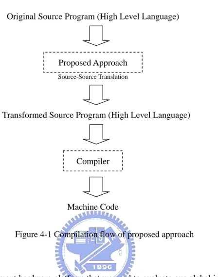
(40) Chapter 4. Simulation and Analysis. In this chapter, we present the simulation results of the proposed approach. First, the experiment methodology and the simulation environment are described. Then the simulation results and the analysis are presented.. 4.1 Simulation Environment In this section, we discuss the simulation environment including the benchmark programs, the compiler parameter, and the hardware platform. Our proposed global integrated approach is implemented by source-to-source translation, in other words, we restructure the original source code to the transformed form, both them are high level languages, like C. We use SUIF as our front-end code analyzer and transformation tool, and GNU C compiler as our back-end code generator. We performed two types of experiments as follows. (1). Execution times: Running the applications on a real machine shows that improving data locality implies increase performance.. (2). Memory hierarchy characteristics: We use a detailed simulation of L1, L2 caches in our systems to show how data locality affects memory hierarchy characteristics such as cache miss rate.. The complete flow of the compilation presented in Figure 2-1.. 31.

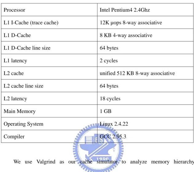
(41) Original Source Program (High Level Language). Proposed Approach Source-Source Translation. Transformed Source Program (High Level Language). Compiler. Machine Code Figure 4-1 Compilation flow of proposed approach. The experiment hardware platform that we used to evaluate our global integrated approach is an x86 Linux platform. We used a 2.4Ghz Intel Pentium4 processor, with 8KB L1 data cache and 512KB L2 unified cache. The processor equipped with 12K L1 trace cache. The benchmark programs we used are compiled using GNU C compiler. The detailed parameters of our platform are given in Table 4-1.. 32.

(42) Table 4-1 Platform used in the experiments to measure execution time Processor. Intel Pentium4 2.4Ghz. L1 I-Cache (trace cache). 12K µops 8-way associative. L1 D-Cache. 8 KB 4-way associative. L1 D-Cache line size. 64 bytes. L1 latency. 2 cycles. L2 cache. unified 512 KB 8-way associative. L2 cache line size. 64 bytes. L2 latency. 18 cycles. Main Memory. 1 GB. Operating System. Linux 2.4.22. Compiler. GCC 2.95.3. We use Valgrind as our cache simulator to analyze memory hierarchy characteristics. The Valgrind distribution includes five useful debugging and profiling tools including Memcheck, Addrcheck, Cachegrind, Massif and Helgrind. Detailed cache profiling can be very useful for analyzing the performance of your program. Valgrind contains Cachegrind which is used as a tool for doing cache simulations. Cachegrind is a cache profiler. It performs detailed simulation of the I1, D1 and L2 caches in your CPU and so can accurately pinpoint the sources of cache misses in your code. It identifies the number of cache misses, memory references and instructions executed for each line of source code, with per-function, per-module and whole-program summaries. It is useful with programs written in any language. Cachegrind runs programs about 20 -- 100x slower than normal. In particular, it records: 33.

(43) (1). L1 instruction cache reads and misses;. (2). L1 data cache reads and read misses, writes and write misses;. (3). L2 unified cache reads and read misses, writes and writes misses.. Cachegrind uses a simulation for a machine with a split L1 cache and a unified L2 cache. This configuration is used for all modern x86-based machines we are aware of. The more specific characteristics of the simulation are as follows. (1). Write-allocate: When a write miss occurs, the block written to is brought into the D1 cache. Most modern caches have this property.. (2). Bit-selection hash function: The line(s) in the cache to which a memory block maps is chosen by the middle bits from M to ( M + N − 1 ) of the M byte address, where: line size = 2 bytes and (cache size / line size) =. 2 N bytes (3). Inclusive L2 cache: The L2 cache replicates all the entries of the L1 cache. This is standard on Pentium chips, but AMD Athlons use an exclusive L2 cache that only holds blocks evicted from L1.. Because Cachegrind can’t simulate trace cache for L1 I-Cache of Intel Pentium4 processor, we described the parameter we used for Cachegrind in Table 4-2.. 34.

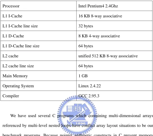
(44) Table 4-2 Platform used in the experiments to simulate cache behavior Processor. Intel Pentium4 2.4Ghz. L1 I-Cache. 16 KB 8-way associative. L1 I-Cache line size. 32 bytes. L1 D-Cache. 8 KB 4-way associative. L1 D-Cache line size. 64 bytes. L2 cache. unified 512 KB 8-way associative. L2 cache line size. 64 bytes. Main Memory. 1 GB. Operating System. Linux 2.4.22. Compiler. GCC 2.95.3. We have used several C programs which containing multi-dimensional arrays referenced by multi-level nested loops have conflict array layout situations to be our benchmark programs. Because pointer arithmetic constructs in C prevent memory layouts transformations by compiler, our benchmark would not use this type of operations to reference data arrays. In order to observe memory hierarchy characteristics, we evaluate performance of proposed global integrated approach using benchmark programs with large input size. The detailed information about benchmark programs are given in Table 4-3.. 35.

(45) Table 4-3 Benchmark programs used in the simulation Program. Code. Description. Matrix. matrix1. 2-dim matrix manipulations. matrix2. 2-dim matrix manipulations. matrix3. 2-dim matrix manipulations. cdft2d. 2-dim Complex Discrete Fourier Transform. rdft2d. 2-dim Real Discrete Fourier Transform. ddct2d. 2-dim Discrete Cosine Transform. ddst2d. 2-dim Discrete Sine Transform. FFT. For each benchmark programs, we experimented with five different versions summarized in Table 4-4.. Table 4-4 Different transformed version used in the simulation Version. Description. original. Compiled without any optimizations. Loop. Compiled with loop transformations. local. Compiled with integrated approach of pure local consideration. global. Our approach: global integrated approach. 4.2 Simulation Results and Analysis In this section, we discuss the simulation results and analyze the execution time and memory hierarchy characteristics of our proposed approach compared with previous research. 36.

(46) 4.2.1 Execution Times We present execution time with varying program size in Figure 4-2. The x-axis represents the problem size from 500 to 2000, the array size is the square of the problem size, and the execution time is the cube of the problem size. The y-axis represents the execution time. From the execution results, we observe that the loop transformations approach and the integrated local approach have similar result; however, our approach has much better results over the previous research.. 1600 1400. Execution time. 1200. original loop local global. 1000 800 600 400 200 0 500 600 700 800 900 1000 1100 1200 1300 1400 1500 1600 1700 1800 1900 2000. Problem size. Figure 4-2 Execution time with varying problem size. We show the speedup of our approach and previous research at Figure 4-3. The results shows that the speedup of our proposed approach is about 26% compared with approach of loop transformations, but the speedup of previous approach is about 7%.. 37.

(47) 1.6 1.4 1.2. Speedup. 1. local. 0.8. global 0.6 0.4 0.2 0. matrix1. matrix2. matrix3. FFT. Figure 4-3 Speedup for the different version of transformations. 4.2.2 Cache Miss Rate The direct effect of improving data locality is to change memory hierarchy characteristics. The cache hit (miss) ratio represents one metric to quantifying data locality. We present cache simulator results of some benchmark programs in Figure 4-4. For the original programs, most array reference falls into L1 cache memory, however, programs with loop transformations exhibit temporal locality in innermost loops so that the data can place in a register. Our approach further improve spatial locality by increase cache hit ratio.. 38.

(48) 100% 90%. Reference percentage. 80% 70%. Memory L2 cache L1 cache Register. 60% 50% 40% 30% 20% 10% 0%. original. loop. local. global. Figure 4-4 Memory reference percentage of different memory hierarchies. Since our global integrated approach only improve spatial locality, both L1 and L2 cache miss rate is further decreased. The detailed L1 and L2 cache miss rate is presented in Figure 4-5.. 39.

(49) 10.00% 9.00% 8.00%. Cache miss rate. 7.00% 6.00%. local global. 5.00% 4.00% 3.00% 2.00% 1.00% 0.00%. L1 typical. L1 large. L2 typical. L2 large. Figure 4-5 Cache miss ratio for L1 and L2 cache. This figure shows the impact of spatial locality affect only L1 cache miss rate, the L2 cache miss rate is unchanged. The reason is the size of L2 cache used in simulation is very large, which is 512 KB.. 4.2.3 Simulation Analysis We suppose that the speedup of our global integrated approach is based on the new program exhibits better data locality. The simulation results show that the transformed program have less L1 cache miss rate, unless L2 cache miss rate unchanged. Suppose L1, L2 cache memory access latency is 2 and 20 cycles, and L1 cache access occupies 40% memory reference, and proposed approach can reduce L1 cache miss rate from 5% to 2%, then the expect value of each L1 access will be reduced from 2.9 cycles to 2.34 cycles. That is 20% reduction, and multiply the frequency 40%, we will get 8% improvement, very approximate to the simulation 40.

(50) results. According to the explanation above, although the locality estimation model is very simple, but it is accurate.. 41.

(51) Chapter 5. Conclusion and Future Works. In this thesis, we present a global integrated compiler framework to improve data locality. Our approach combines loop and data transformations, based on a new locality model and simple linear algebra techniques. Our proposed locality model uses reference distance as a metric of the quality of data locality. To representing data locality characteristics in a loop nest, we use the concept of a stride vector. Then a cost function derived from a stride vector is presented to quantify different occurrences of array references. Our approach divides the compiler framework into two stages: (1) local transformation selection stage; and (2) global transformation decision stage. We use this mechanism to resolve conflict situation of pure local approach. When considering loop and data transformations simultaneously, our approach specializes in the loop transformations for optimizing temporal locality. Once the potential temporal locality is exploited, our approach uses data transformations to exploit potential spatial locality in a loop nest. The main difference between our research and previous research is our techniques focuses on the correlation between different loop nests and between different types of data locality, in other words, how the integrated approach can be adapted to work with multiple loop nests. Simulation results shows our integrated approach does make a difference, and improves over techniques based on pure loop or pure data transformations. Moreover, the proposed global consideration improves over previous pure local consideration. The information required by the compiler to apply our techniques is easily 42.

(52) obtained during dependence analysis, which is performed by almost every optimizing compiler. Once the information is obtained, our approach uses simple linear algebraic techniques to manipulate loop nests and array references. This technique can be applied to any architecture with a memory hierarchy. There are still several researches could be further studied. An important future direction is to consider non-linear transformations to restructuring code. The impact of non-linear transformations merits further investigation. Another important question is whether or not data transformation can be applied on low level of compilation process. Transforming memory layouts at code generation phase, not at source level, is a challenging task.. 43.

(53) References [1] U. Banerjee. Unimodular transformations of double loops. In Advances in Languages and Compilers for Parallel Processing, edited by A. Nicolau et al., MIT Press, 1991. [2] S. Carr, K. McKinley, and C.-W. Tseng. Compiler optimizations for improving data locality. In Proc. the 6th International Conference on Architectural Support for Programming Languages and Operating Systems, pages 252–262, October 1994. [3] M. Cierniak, and W. Li. Unifying data and control transformations for distributed shared memory machines. In Proc. SIGPLAN ’95 Conference on Programming Language Design and Implementation (PLDI), June 1995. [4] D. Gannon, W. Jalby, and K. Gallivan. Strategies for cache and local memory management by global program transformations. Journal of Parallel and Distributed Computing, 5:587–616, 1988. [5] M. Kandemir, A. Choudhary, J. Ramanujam, and P. Banerjee. Improving locality using loop and data transformations in an integrated framework. In Proc. International Symposium on Microarchitecture, December, 1998. [6] M. Kandemir, A. Choudhary, N. Shenoy, P. Banerjee, and J. Ramanujam. A hyperplane based approach for optimizing spatial locality in loop nests. In Proc. 12th ACM International Conference on Supercomputing, 1998. [7] M. Kandemir, J. Ramanujam, and A. Choudhary. Compiler algorithms for optimizing locality and parallelism on shared and distributed memory machines. In Proc. 1997 Int. Conf. Parallel Architectures and Compilation Techniques (PACT 97), pages 236–247, San Francisco, CA, November 1997. [8] S-T. Leung, and J. Zahorjan. Optimizing data locality by array restructuring. Technical Report TR 95-09-01, CSE Dept., University of Washinton, 1995. [9] W. Li. Compiling for NUMA parallel machines. Ph.D. Thesis, Cornell University, 1993. [10] M. O’Boyle, and P. Knijnenburg. Non-singular data transformations: Definition, validity, applications. In Proc. 6th Workshop on Compilers for Parallel Computers (CPC 96), pages 287–297, Aachen, Germany, 1996. [11] A. Schrijver. Theory of linear and integer programming, John Wiley, 1986. [12] M. Wolf and M. Lam. A data locality optimizing algorithm. In Proc. ACM SIGPLAN 91 Conf. Programming Language Design and Implementation, pages 30–44, June 1991. [13] M. Wolfe. High Performance Compilers for Parallel Computing, Addison-Wesley Publishing Company, 1996. 44.

(54)