Time-constrained distributed program reliability analysis

891

Short Paper

Time-Constrained Distributed Program

Reliability

Analysis

DENG-JYI CHEN , MING-SANG CHANG, MING-CHENG SHENG* AND MAW-SHENG HORNG**

Institute of Computer Science and Information Engineering National Chiao Tung University

Hsinchu, Taiwan 300, R.O.C. *Department of Information Management National Ping Tung Institute of Commerce

Ping Tung, Taiwan 912, R.O.C.

**Department of Mathematics and Science Education National Taipei Teachers College

Taipei, Taiwan 106, R.O.C.

In this paper, we propose an approach to the reliability analysis of distributed programs that addresses real-time constraints. Our approach is based on a model for evaluating transmission time, which allows us to find the time needed to complete execution of the program, task, or mission under evaluation. With information on time-constraints, the corresponding Markov state space can then be defined for reliability computation. To speed up the evaluation process and reduce the size of the Markov state space, several dynamic reliability-preserving reductions are developed. A simple distributed real-time system is used as an example to illustrate the feasibility and uniqueness of the proposed approach.

Keywords: distributed program reliability, distribute system reliability, file spanning

tree, file spanning forest, reliability.

1. INTRODUCTION

Distributed real-time systems have been widely applied in various application domains, including the military, industrial manufacturing, and medical care sectors. Numerous research projects related to distributed real-time systems have been conducted in the past two decades [13-18]. Reliability analysis is an important issue in designing distributed real-time systems for various applications. In distributed computing systems, distributed program reliability has been proposed as a reliability index for analyzing the probability of successful execution of a program, task, or mission in a system. Distributed program reliability (DPR) [1-3] in a distributed computer system (DCS) is defined as the probability that the program under

con-Received October 3, 1996; accepted June 27, 1997. Communicated by Shing-Tsaan Huang.

1_{The early-version of this paper has been presented on the Fifth IEEE Symposium on Parallel and}

Distributed Processing, Dallas, Texas. This research was supported in part by the National Science

sideration with distributed files can be run successfully in spite of some faults occurring in the processing elements or in the communication links. In [1], Prasanna Kumar et al. introduced the notions of a File Spanning Tree (FST), Minimal File Spanning Tree (MFST), and File Spanning Forest (FSF). An FST is defined as a spanning tree that connects the root (the PE that runs the program under consid-eration) to some other nodes such that its vertices hold all the files required to execute that program. An MFST is an FST such that there is no other FST which is a subset of it. An FSF is defined in the same way as an FST except that the union of all the data files associated with evaluated distributed programs is accomplished before the spanning tree is identified.

Under the FST concept, several reliability evaluation algorithms have been developed to speed up the reliability evaluation process [4-8]. However, reliability models so far proposed for distributed program reliability evaluation do not capture the effect of real-time constraints. In this paper, we propose an approach to reliability performance analysis of distributed programs that addresses the real-time con-straint issue. The approach proposed here is based on a model for evaluating transmission time to find the time needed to complete execution of the FST for a given program, task, or mission. With time-constraint information and the ex-ecution time of every FST, the corresponding Markov state space can be defined for reliability computation. To speed up the evaluation process and reduce the size of the Markov state space, several dynamic reliability-preserving reduction tech-niques are developed. A simple distributed real-time system is used as an example to illustrate the feasibility and uniqueness of the proposed approach.

2. TIME-CONSTRAINED DISTRIBUTED PROGRAM

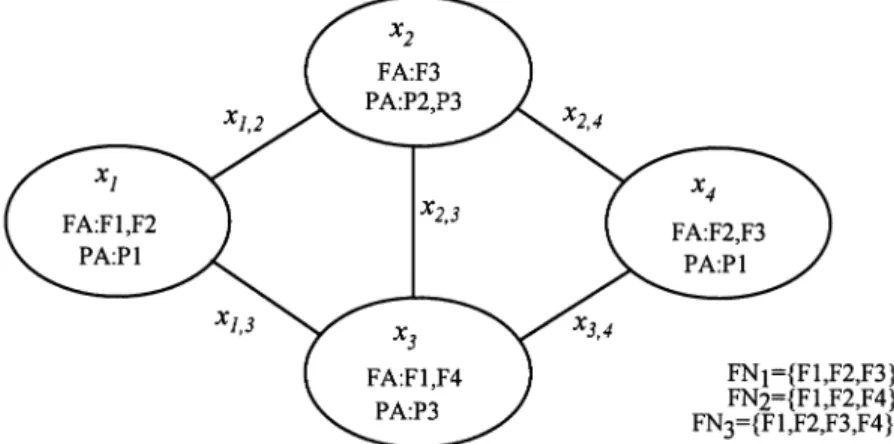
Consider the distributed processing system in Fig. 1. There are four process-ing elements (x1, x2, x3, x4) connected by links x1,2, x1,3, x2,3, x2,4 and x3,4. Processing

element x1 contains two data files (F1 and F2) and can run program P1 directly to

communicate with other nodes and access data files required to complete the

execution of program P1. The information in each node in Fig. 1 is summarized by FAj, PAj(j = 1, 2, 3, 4), and FNi(i = 1, 2, 3), where FAi is the set of data files

available at processing element xi, PAj is the set of programs, tasks, or missions

available at processing element xj, and FNi is the set of data files needed

for program Pi to be executed.

Let the execution of P1 in the DCS in Fig. 1 require the use of F1, F2, and F3 and allow P1 to be run from either node x1 or node x4. From the DCS graph,

we can identify the following File Spanning Trees (FSTs) rooted on x1:

1) x1 x2 x1,2, 2) x1 x2 x3 x1,2 x2,3, 3) x1 x2 x4 x1,2 x2,4,

4) x1 x2 x3 x1,3 x2,3, 5) x1 x3 x4 x1,3 x3,4, 6) x1 x2 x3 x4 x1,2 x2,3 x3,4,

7) x1 x2 x3 x4 x1,2 x2,4 x3,4, 8) x1 x2 x3 x4 x1,3 x2,3 x2,4, and

9) x1 x2 x3 x4 x1,3 x3,4 x2,4.

A time-constrained system is a system whose computations and actions must be performed before a given deadline [9-10]. For a real-time system, the deadline is crucial. The system must be able to perform and meet critical deadlines even when it is not fully operational because of abnormal conditions in its components. Some FSTs may be unable to meet the deadline constraints. Such FSTs will be considered to fail during reliability measurement even though the system is still operational.

When a time constraint is considered, it may turn out that some of the FSTs identified in Fig. 1 are unable to complete execution before the deadline. We consider such FSTs to be failed FSTs; they are classified as being in failure states. Thus, three steps must be performed before we can compute the reliability of a program which is being evaluated. We must

1) generate all the FSTs associated with the evaluated distributed program, 2) evaluate the transmission time of each FST and identify the failed FSTs,

and

3) map the good FSTs into Markov transition states and the failed FSTs into failure states.

Thus, the state space of the Markov model can be partitioned into two sets: 1) the set O of operational states, which contain at least one FST each and meet the time constraint, and 2) the set F of failure states, which either contain no FSTs or do not meet the time deadline. When time constraints are used, two new reliability measures for the DCS can be derived as follows.

Definition 1: The Time-Constrained Distributed Program Reliability (TCDPR) of

the model can be defined as TCDPR =

Σ

S∈O (t) where Ps(t) is the state probability

for state S and O is the set of states that contain at least one FST and allow the program in the DCS to meet the execution deadline.

Definition 2: The Time-Constrained Distributed System Reliability (TCDSR) can

be defined as TCDSR =

Σ

and O is the set of states that contain at least one File Spanning Forest (FSF) and allow all programs in the DCS to meet their deadlines.

3. RELIABILITY EVALUATION OF TIME-CONSTRAINED DISTRIBUTED PROGRAMS

In this section, we will present an approach to reliability evaluation of time-constrained distributed programs. As discussed in the previous section, three steps must be performed before the TCDPR can be computed. The first step is to generate all the FSTs associated with the program under evaluation. This can be done using the algorithms presented in [1,4,5]. The next step is to evaluate the transmission time of each FST and identify the failed FSTs. To evaluate the transmission time of each FST, we shall propose a model for evaluating the response time of DCSs connected to a wide area network. In our model, we assume that there are two processors: the application processor, which executes programs, and the network processor, which handles all the intra- and internode communications in a DCS node. The execution time of a program is assumed to be constant in our model, and the time needed to transfer needed files from resident nodes to the root node is considered to be the response time. Many factors affect the response time, including link capacity, network topology, file distribution, and CPU speed. CPU speed is often less important than the other factors [11]. Once the transmission time of each FST is computed, we can map the successful FSTs into operational states and the failed FSTs or non-FSTs (FSTs that cannot meet the deadline for execution or subtrees that are not FSTs) into failure states in the resulting Markov process. Finally, we apply a common technique for solving the Markov process described in [12] to compute the reliability as a function of time and MTTF. In the following sections, we present the file transfer protocol used in our evaluation model, the transmission time evaluation algorithm used to compute the response time, and the complete method for computing the TCDPR and TCDSR.

3.1 File Transfer Protocol

At beginning of each cycle, the root node sends the file request signal REQ to all of its neighboring nodes. The node receiving the REQ signal will send the requested file through the communication link, and then file request signals for the remaining files will be issued to the neighboring nodes. The transmission time of the REQ signal is assumed to be fixed and very small, so it can be neglected. In this model, we assume that a simple store-forward scheme and a virtual cut-through [12] mechanism are used. In virtual cut-through, packets arriving at an intermediate node are forwarded to the next node in the route without buffering. A node that has data coming from more than one neighboring node is called a branch node. The data packets received by branch nodes are sent according to a predefined priority.

for all node xi do

repeat

if self_demand(REQ) then

add_send_request(Vt, REQ)

for all neighboring node of xi (denoted as xj) do

if send_request(xj) ≠∅

then send_request(xj)

if receive_request_from(xj, REQ)

then if REQ has been processed then discard REQ else

add_send_list(xj, FAi∩ REQ)

add_send_request(Vt-xj, REQ-FAi)

if receive_data_from(xj, DATA, xk) then

if xk = xi then save DATA

else if status_channel_to(xk) = idle

pass_to(xk, DATA)

else

save_data(TEMP) add_send_list(xk, TEMP)

if status_channel_to(xk) = idle and send_list(xj) ≠ ∅ then

send_data_to(xk)

od until ∅ od

3.2 Response Time Evaluation Algorithm

The Transmission Time algorithm developed here is based on traversing the DCS graph in a breadth-first manner. A marking strategy is used to eliminate the possibility of visiting a node more than once. The algorithm begins by choosing one node as a root to generate file transmission paths from the set of nodes which includes the program under consideration. Starting from this root, paths are gen-erated by connecting edges to this root or to the paths expanded from this root;

t.node is, therefore, needed to hold the necessary information about this root; t.path

is used to hold the nodes included in path t; and t.req is used to hold the message of the file request signal.

The procedure for constructing the file transmission paths consists of a checking step and an expanding step. In the checking step, the subgraphs that have been generated so far, which are stored in a list called TRY, are checked to determine whether they are file transmission paths. A subgraph t is a file trans-mission path if its t.node contains files required to execute the distributed program, that is, if FAt.node∩ t.req ≠ ∅. If the t.node contains all the files required,

then no more file request signals will be sent to the neighboring nodes that have not been visited. Thus, subgraph t is removed from TRY if FAt.node⊃ t.req. Once

the checking process is complete, the list TRY will contain all the paths in which

t.req is not an empty set.

to a new adjacent vertex in the hope that the new vertex will have the needed files (if TRY is empty, of course, the algorithm stops). The adjacent vertex added might have all or some of the needed files. If the added node contains some of the missing files, a new file transmission path is generated by connecting this adjacent vertex to the existing path. If none of the needed files are in the adjacent vertex, then this node can be used as an intermediate node to access another set of adjacent nodes in the next expanding step. If t.node has more than one unvisited adjacent vertex, a flag t.node.branch is set to indicate that this node is a branching node.

Once the file transmission paths are generated, information on link capacities and file sizes is used to generate the real paths. Before the real paths are generated, the file transmission paths are sorted by a predefined order of priority for branch nodes. A real path contains a pair of lists: one lists the amount of data that will be sent from each node, and the other lists the capacity of the links in the path. The mapping from a file transmission path to a real path is straightforward. First, the amount of the data sent from the last node is accumulated in the variable x.acc. Then, for path xp1, xp2, …, xpm, two lists are generated: xp2.acc, xp3.acc, …, xpm.acc

and newr.capacity = (cap(xp1, xp2), cap(xp2, xp3), …, cap(xpm–1, xpm)), where m is the

number of nodes in the path, xpi (i = 1, 2, …, m) is nodes in the path, xpi.acc (i =

1, 2, …, m) is the accumulated data to be transmitted for node xpi, cap(xpi, xpi+1)

(i = 1, 2, …, m-1) is the link capacity between nodes xpi and xpi+1, and newr is a

new real path. The formal algorithm is stated below.

The transmission time for files to pass through a real path can be calculated recursively. If the path length is equal to 1, the transmission time can be computed directly by dividing the amount of data by the capacity of the link. If the time needed to empty the nodes in each path forms a descending order from the last node to the root node, Fn

Cn > Fn – 1 Cn – 1– Cn > Fn – 2 Cn – 2– Cn – 1 > … > F1 C2– C1

, then the transmission time is Fn

Cn

, where Fi (i = 1, 2, …, n) is the file size in node i and Ci (i = 1, 2, …,

n) is the link capacity between node i and node i+1. The cut-through mechanism indicates that if a node exists that is empty before the data in its neighboring node goes through, then the link between these two nodes can be eliminated.

Once the transmission time through various paths of each file needed has been computed, the response time can be obtained by 1) finding the minimum transmission time for each file needed and 2) finding the maximum of the trans-mission times obtained in 1). A formal description of the algorithm is given below.

Transmission Time Evaluation Algorithm Step 1: Initialization

t.node = first node xj which includes the program to be executed. t.path = xj t.requ = FNj visit = {xj} add t to TRY PATH = ∅ REALPATH = ∅

Step 2: Generating all file transmission paths

repeat

2.1 Checking step and Generating path

for all t ∈ TRY do

if FAt.node∩ t.req ≠ ∅ then newp.file = FAt.node∩ t.req newp.path = t.path

add newp to PATH

if FAt.node⊃ t.req then

remove t from TRY

od

2.2 Expanding Step NEW = ∅

for all t ∈ TRY do

add EXPAND(t) to NEW

od

TRY = NEW

until TRY = ∅

Step 3: Generating all real paths

sort the paths in the path list PATH

for all p ∈ PATH do

for all Fi∈ p.file do newr.file = Fi

MAP_TO_REAL(p.path, Fi)

add newr to REALPATH

od

ACC(p.path)

od

Step 4: Time Evaluation

for all r ∈ REALPATH do

time =TIME_EVALUATE(r.capacity, r.size)

if time < r.file.time then

r.file.time = time

od

function EXPAND(t)

begin

count = 0

for all node xi adjacent to t.node and xi∉ visit do

begin

newt.node = xi newt.path = t.path+xi newt.requ = t.requ-FAt.node

add newt to tmp add xi to visit count = count + 1 if count > 1 then t.node.branch = true end

od

EXPAND = tmp

end. (*EXPAND*)

function MAP_TO_REAL(xp1, xp2, …, xpm, File)

begin

xpm.acc = xpm.acc+size(File)

newr.size = (xp1.acc, xp2.acc, …, xpm.acc)

newr.capacity = (cap(xp1, xp2), cap(xp2, xp3), …, cap(xpm-1, xpm)) end

(*MAP_TO_REAL*)

function ACC(xp1, xp2, …, xpm)

begin

for all branching nodes xpj do

xpj.acc = xpj.acc+

Σ

if j is the largest index such that Fj

Cj– Cj + 1 ≤ Fj – 1 Cj – 1– Cj then TIME_EVALUATE((C1, C2, …, Cj-1, Cj+1, …, Cn-1); (F1, F2, …, Fj-1, Fj, …, Fn)) end(*TIME_EVALUATE*)

3.3 An Example of Response Time Evaluation

Fig. 2 shown the DCS with the capacity of each communication link specified. Suppose we want to compute the response time of distributed program 1 when link 3 is down. Based on the Response Time Evaluation algorithm, we get four file transmission paths: 1) F2: x1x2, 2) F4: x1x2, 3) F3: x1x3, and 4) F4: x1x3. These

file transmission paths and the real paths generated are shown in Fig. 3. The Time Evaluation function calculates the response time of program 1 to be 60ms.

For the state S = {1, 3}, three file transmission paths are generated for F2, F3, and F4 for program 1. These file transmission paths and the real paths generated from them are shown in Fig. 4. With these real paths, the computed response time of program 1 is 140ms.

Fig. 2. The distributed computer system with file size and link capacity specified.

Fig. 3. The path list and real path list for S = {3}.

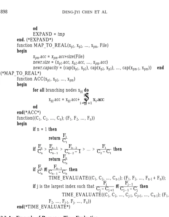
By applying the Transmission Time algorithm to all the FSTs generated for distributed program 1, we obtain the response time of each FST, as shown in Fig. 5. State {i, j} represents the state where both link i and link j have failed while State {i} represents a failure in link i. State ∅ indicates that all the links are working.

Suppose we set the deadline for distributed program 1 at 100ms. Then, states {1} {1, 3} {1, 4} {1, 5} and {1, 4, 5} become failure states; although they are operational, they fail to meet the execution deadline. The set of failure states can be collapsed into one large failure state F; the resulting Markov Chain is shown in Fig. 6.

3.4 Time-Constrained Distributed Program Reliability Evaluation

Once the state space is obtained, the transition probability between states can be supplied by reliability engineers. Method 1 describes the process used to compute TCDPR and TCDSR.

Method 1: TCDPR and TCDSR Analysis

Step 1: Generate the FSTs of the evaluated distributed program.

Step 2: Use the Transmission Time algorithm to evaluate the execution time of each FST.

Step 3: Map each FST into the corresponding Markov state and merge all failure FSTs into one failure state.

Step 4: Assign a transition probability ri (or failure probability) to each transition.

Step 5: Generate the transition probability matrix P.

Step 6: Analyze the resulting Markov model to find the reliability, mean time to failure, etc.

In the following, we will present the complete computation of the TCDPR of distributed program 1 from the last section (Fig. 2).

Example: Compute the TCDPR1 of the DCS shown in Fig. 2 without a repair

mechanism.

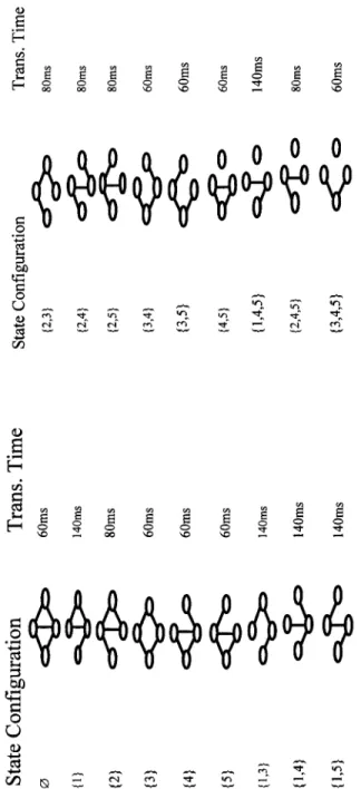
Applying Method 1, we obtain the Markov model shown in Fig. 6. Assume that the failure probabilities associated with the set of communication links e1, e2,

…, e5 in the DCS of Fig. 2 is ρ1, ρ2, …, ρ5, where ρi = λi∆t (i = 1, 2, …, 5). For

the purposes of this example, we set the transition probability as λ1∆t = λ2∆t = …

= λ5∆t = 0.01. The reliability parameters λj are assumed to be provided by r

eliability engineers. The resulting transition matrix P is shown in Table 1.

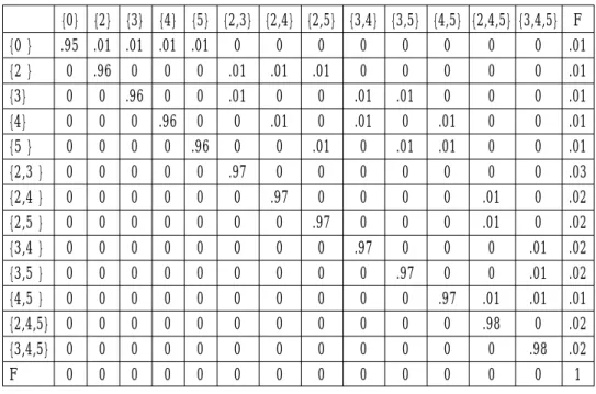
Table 1. The transition probability matrix P for the resulting Markov Chain.

{0} {2} {3} {4} {5} {2,3} {2,4} {2,5} {3,4} {3,5} {4,5} {2,4,5} {3,4,5} F {0 } .95 .01 .01 .01 .01 0 0 0 0 0 0 0 0 .01 {2 } 0 .96 0 0 0 .01 .01 .01 0 0 0 0 0 .01 {3} 0 0 .96 0 0 .01 0 0 .01 .01 0 0 0 .01 {4} 0 0 0 .96 0 0 .01 0 .01 0 .01 0 0 .01 {5 } 0 0 0 0 .96 0 0 .01 0 .01 .01 0 0 .01 {2,3 } 0 0 0 0 0 .97 0 0 0 0 0 0 0 .03 {2,4 } 0 0 0 0 0 0 .97 0 0 0 0 .01 0 .02 {2,5 } 0 0 0 0 0 0 0 .97 0 0 0 .01 0 .02 {3,4 } 0 0 0 0 0 0 0 0 .97 0 0 0 .01 .02 {3,5 } 0 0 0 0 0 0 0 0 0 .97 0 0 .01 .02 {4,5 } 0 0 0 0 0 0 0 0 0 0 .97 .01 .01 .01 {2,4,5} 0 0 0 0 0 0 0 0 0 0 0 .98 0 .02 {3,4,5} 0 0 0 0 0 0 0 0 0 0 0 0 .98 .02 F 0 0 0 0 0 0 0 0 0 0 0 0 0 1

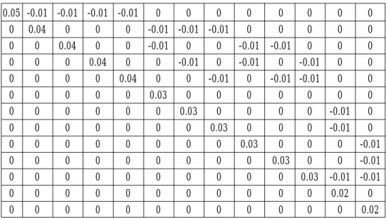
The 14-state Markov chain consists of one absorbing state and 13 transient states. The inverse of the fundamental matrix (I-Q) is shown in Table 2, and the fundamental matrix M [12] is shown in Table 3.

Fig. 7 shows reliability as a function of time after computation; the reliability of failure only and failure-repair cases is also shown in Fig. 7.

In Table 4, The DCS uses about 70 time units in transient states (starting in a state where all the communication links are good before entering failure state F). Hence, when it starts under perfect conditions, the mean time to failure (MTTF) is 70.00001 time units; when it starts at state {2} (link 2 failed), it is 58.33334 time units, and so on.

Table 2. The inverse of the fundamental matrix (I-Q). 0.05 -0.01 -0.01 -0.01 -0.01 0 0 0 0 0 0 0 0 0 0.04 0 0 0 -0.01 -0.01 -0.01 0 0 0 0 0 0 0 0.04 0 0 -0.01 0 0 -0.01 -0.01 0 0 0 0 0 0 0.04 0 0 -0.01 0 -0.01 0 -0.01 0 0 0 0 0 0 0.04 0 0 -0.01 0 -0.01 -0.01 0 0 0 0 0 0 0 0.03 0 0 0 0 0 0 0 0 0 0 0 0 0 0.03 0 0 0 0 -0.01 0 0 0 0 0 0 0 0 0.03 0 0 0 -0.01 0 0 0 0 0 0 0 0 0 0.03 0 0 0 -0.01 0 0 0 0 0 0 0 0 0 0.03 0 0 -0.01 0 0 0 0 0 0 0 0 0 0 0.03 -0.01 -0.01 0 0 0 0 0 0 0 0 0 0 0 0.02 0 0 0 0 0 0 0 0 0 0 0 0 0 0.02

Table 3. The fundamental matrix M = (I-Q)–1_.

20 5 5 5 5 3.3 3.3 3.3 3.3 3.3 3.3 5 5 0 25 0 0 0 8.3 8.3 8.3 0 0 0 8.3 0 0 0 25 0 0 8.3 0 0 8.3 8.3 0 0 8.3 0 0 0 25 0 0 8.3 0 8.3 0 8.3 8.3 8.3 0 0 0 0 25 0 0 8.3 0 8.3 8.3 8.3 8.3 0 0 0 0 0 33.3 0 0 0 0 0 0 0 0 0 0 0 0 0 33.3 0 0 0 0 16.6 0 0 0 0 0 0 0 0 33.3 0 0 0 16.6 0 0 0 0 0 0 0 0 0 33.3 0 0 0 16.6 0 0 0 0 0 0 0 0 0 33.3 0 0 16.6 0 0 0 0 0 0 0 0 0 0 33.3 16.6 16.6 0 0 0 0 0 0 0 0 0 0 0 50 0 0 0 0 0 0 0 0 0 0 0 0 0 50

To compute the TCDSR, one needs to generate FSFs instead of FSTs. The concept of generating FSFs was introduced in [1]. Once all the FSFs are obtained, the TCDSR can be computed using Method 1.

Table 4. MTTF for each state.

start state time unit

state ∅ 70.00001 state {2} 58.33334 state {3} 58.33334 state {4} 66.66669 state {5} 66.66669 state {2,3} 33.33337 state {2,4} 50.00007 state {2,5} 50.00007 state {3,4} 50.00007 state {3,5} 50.00007 state {4,5} 66.66669 state {2,4,5} 50.00005 state {3,4,5} 50.00005

4. DYNAMIC RELIABILITY PRESERVING REDUCTIONS

In this section, we will propose dynamic reliability-preserving reduction tech-niques to reduce the size of graph G and, therefore, reduce the state space of the associated Markov process model. These reduction techniques are listed below.

1) Degree-1 Reduction

Degree-1 reduction is used to eliminate nodes that contain no data files needed by the program under consideration.

Definition 3: Let xi,j be an edge in G such that degree(xi) = 1 and FAi∩ FN = ∅

and PAi∩ PN = ∅. Then, G’ is obtained by deleting xi,j and xi.

2) Series Reduction

Like degree-1 reduction, series reduction can be used for real time DCS reliability problems. There are some differences between using series reduction in DCS reliability problems and using it in real time DCS reliability problems. Series reduction for the real time DCS reliability problems can be defined as follows.

Definition 4: Let xi,j and xi,k be two edges in G such that degree(xi) = 2 and FAi

∩ FN = ∅ and PAi∩ PN = ∅. Then G’ is obtained by replacing xi,j and xi,k with

a single edge xj,k such that λi,k = λi,j + λi,k, where λi,j and λi,k are the failure rates

of edges xi,j and xi,k, respectively. The capacity of edge xj,k, cj,k = Min(ci,j, ci,k), where

ci,j and ci,k are the capacities of edges xi,j and xi,k respectively.

In other words, if degree (xi) = 2 and node xi contains no needed data files

or programs, then we can apply series reduction on G.

3) Degree-2 Reduction

In dynamic reliability analysis, degree-2 reduction can be applied to reducible nodes for real time reliability analysis. Suppose node xi is a reducible node. Then,

one can apply series reduction to node xi and move data files and programs within

node xi to one of its adjacent nodes, xj or xk. This reduction case is called

degree-2 reduction.

By using dynamic reliability preserving reduction, Method 1 proposed in section 3.4 can be modified to reduce the state space. Method 2 presents the complete approach.

Method 2: TCDPR and TCDSR analysis for the DCS based on Reliability-Preserving

Reductions.

Step 1: Perform degree-1 reduction, series reduction, and degree-2 reduction on DCS graph G to obtain the reduced graph G’.

Step 3: Use the Transmission Time algorithm to evaluate the execution time of each FST.

Step 4: Map each FST into the corresponding Markov state and merge all failure FSTs into one failure state.

Step 5: Assign a transition probability λi (or failure probability) to each transition.

Step 6: Generate the transition probability matrix P.

Step 7: Analyze the resulting Markov model to find the reliability, mean time to failure, etc.

Example

To compute the TCDPR1 of the DCS shown in Fig. 1, we apply Method 2.

The DCS graph G can be reduced by using series reduction on e4 and e5. Let the

edge generated by series reduction be e45, with ρ4,5 = ρ4 + ρ5. The resulting

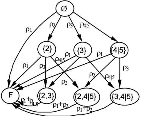
Markov process is shown in Fig. 8, where state {4|5} indicates that either link 4 or link 5 has failed.

Fig. 8. The Markov chain for computing TCDPR1 after reduction of the DCS in Fig. 1.

Assume that the failure probabilities associated with the set of communication links e1, e2, …, e5 in the DCS of Fig. 2 is ρ1, ρ2, …, ρ5. To present an example,

we set λ1∆t = λ2∆t = … = λ5∆t = 0.01. The resulting transition matrix P is shown

Table 5. The transition matrix for the resulting Markov process. states {0} {2} {3} {4|5} {2,3} {2,4|5} {3,4|5} F ∅ .95 .01 .01 .02 0 0 0 .01 {2} 0 .96 0 0 .01 .02 0 .01 {3} 0 0 .96 0 .01 0 .02 .01 {4|5} 0 0 0 .97 0 .01 .01 .01 {2,3} 0 0 0 0 .97 0 0 .03 {2,4|5} 0 0 0 0 0 .98 0 .02 {4|5} 0 0 0 0 0 0 .98 .02 F 0 0 0 0 0 0 0 1

The 8-state Markov chain consists of one absorbing state and 7 transient states. The inverse of the fundamental matrix and the fundamental matrix is shown in Tables 6 and 7, respectively.

Table 6. The inverse of the fundamental matrix of the resulting Markov process.

0.05 -0.01 -0.01 -0.02 0 0 0 0 0.04 0 0 -0.01 -0.02 0 0 0 0.04 0 -0.01 0 -0.02 0 0 0 0.03 0 -0.01 -0.01 0 0 0 0 0.03 0 0 0 0 0 0 0 0.02 0 0 0 0 0 0 0 0.02

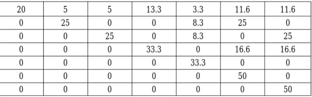
Table 7. The fundamental matrix of the resulting Markov process.

20 5 5 13.3 3.3 11.6 11.6 0 25 0 0 8.3 25 0 0 0 25 0 8.3 0 25 0 0 0 33.3 0 16.6 16.6 0 0 0 0 33.3 0 0 0 0 0 0 0 50 0 0 0 0 0 0 0 50

Fig. 9. Reliability as a function of time using Method 2.

Table 8. MTTF for each state.

start state time unit

state ∅ 70.00003 state {2} 58.33334 state {3} 58.33334 state {4|5} 33.33337 state {2,3} 66.66676 state {2,4|5} 50.00005 state {3,4|5} 50.00005 5. CONCLUSIONS

Reliability analysis is an important issue in designing distributed real-time systems for various applications. If an appropriate reliability index is not available to guide the design of a system, the performance of the system may be unable to meet the reliability requirements of its particular application domain, and modifying the system to the desired level of reliability may be costly. Systems that do not meet Fig. 9 and Table 8 show reliability as a function of time and MTTF. The reliability obtained from Method 2 is exactly the same as that obtained from Method 1 (in Fig. 6). Also, the MTTF starts at state .

appropriate reliability standards can result in loss of business or even life-threatening catastrophes in applications such as nuclear power plant control. Current models for evaluation of distributed program reliability do not capture the effect of real-time constraints. In this paper, we have proposed an approach to analyzing the reliability performance of distributed programs that addresses the issue of real-time constraints. Examples have been given in which reliability is computed as a function of time and the MTTF of the evaluated distributed program.

REFERENCES

1. V. K. Prasanna Kumar, S. Hariri and C. S. Raghavendra, “Distributed program reliability analysis,” IEEE Transactions on Software Engineering, Vol. 12, No. 1, 1986, pp. 42-50.

2. A. Kumar, S. Rai, and D. P. Agrawal, “On computer communication network reliability under program execution constraints,” IEEE Journal of Selected

Areas Communication, Vol. 6, No. 8, 1988, pp 1393-1399.

3. A. Kumar, S. Rai, and D. P. Agrawal, “Reliability evaluation algorithms for distributed systems,” in Proceedings of IEEE INFOCOM 88, 1988, pp. 851-860. 4. Deng-Jyi Chen and T. H. Huang, “Reliability analysis of distributed systems based on a fast reliability algorithm,” IEEE Transactions on Parallel and

Dis-tributed Systems, Vol. 3, No. 2, 1992, pp. 139-154.

5. Deng-Jyi Chen and M. S. Lin, “On distributed computing systems reliability analysis under program constraints,” IEEE Transactions on Computer, Vol. 43, No. 1, 1994, pp. 87-97.

6. C. S. Raghavendra, V. K. Prasnna Kumar, and S. Hariri, “Reliability analysis in distributed system,” IEEE Transactions on Computer, Vol. 37, No. 3, 1988, pp. 352-358.

7. M. S. Lin and D. J. Chen , “Distributed program reliability analysis,” in IEEE

Computer Society 3rd Workshop on Future Trends on Distributed Computing Systems, 1992, pp. 395-401.

8. Anup Kumar and Dharma P. Agrawal “A generalized algorithm for evaluat-ing distributed program reliability,” IEEE Transactions on Reliability, Vol. 42, No. 3, 1993, pp. 416-426.

9. J. A. Stankovic, “A perspective on distributed computer systems,” IEEE

Trans-actions on Computer, Vol. 33, No. 12, 1984, pp. 1102-1115.

10. J. A. Stankovic, “Misconceptions about real-time computing,” Computer, Vol. 21, No. 10, 1988, pp. 10-19.

11. D. J. Chen, “Reliability evaluation in distributed real-time systems,” Modern

Engineering and Technology Seminar, 1992, pp. 243-274.

12. U. N. Bhat, Elements of Applied Stochastic Processes, 2nd ed., New York, John Wiley, 1984.

13. P. Kermani and L. Kleinrock, “Virtual cut-through: A new computer com-munication switching technique,” Computer Networks, Vol. 3, No. 5, 1979, pp. 267-286.

14. T. C. K. Chou and J. A. Abraham, “Load redistribution under failure in dis-tributed systems,” IEEE Transactions on Computer, Vol. 32, No. 9, 1983, pp. 799-780.

15. D. W. Davies, E. Holler, E. D. Jensen, S. R. Kimbleton, B. W. Lampson, G. Lelann, K. J. Thurber and R. W. Watson, Distributed Systems — Architecture

and Implementation, Springer-Verlag, 1981.

16. P. Enslow, “What is a distributed data processing system,” Computer, Vol. 11, No. 1, 1978, pp. 13-21.

17. J. Garcia-Molina, “Reliability issues for fully replicated distributed database”,

Computer, Vol. 15, No. 2, 1982, pp. 34-42.

18. A. Satyanarayna and J. N. Hagstrom, “New algorithm for reliability analysis of multiterminal networks,” IEEE Transactions on Reliability, Vol. 30, 1981, pp. 325-333.

Deng-Jyi Chen received the B.S. degree in computer science from Missouri State University, Cape Girardeau, and the M.S. and Ph.D. degrees in computer science from the University of Texas, Arlington, in 1983, 1985, and 1988, respectively. He is a professor at National Chiao Tung University, Hsinchu, Taiwan. Prior to joining the faculty of National Chiao Tung University, he was with National Cheng Kung University, Tainan, Taiwan, and the Unite Company, Fort Worth, TX. His interests include object-oriented computing, software reuse, reliability and performance evaluation of distributed systems, computer networks, and fault-tol-erant systems.

Ming-Sang Chang received the B. S. degree in Electronic Engineer-ing from National Taiwan University of Science and Technology, Taipei, Taiwan and the M.S. degree in information engineering from TamKang University in 1979, 1982 , respectively. He is currently working toward a Ph.D. degree in the Department of Computer Science and Information Engineering, National Chiao Tung University, Hsichu, Taiwan. His research interests include computer network, distributed systems, and reliability evaluation.

Ming-Cheng Sheng received the B.S. degree in communication en-gineering and the M. S. degree in computer enen-gineering from National Chiao Tung University, Hsinchu, Taiwan, in 1979 and 1985, respectively. From 1987 to 1988, he was a visiting scientist at the IBM T. J. Watson Research Center, New York. He also received the Ph.D. degree in computer science and information engineering from National Chiao Tung University in 1992. In August 1993, he joined the National Ping Tung Institute of Commerce, Ping Tung, Taiwan. Since then, he has been an associate professor of information management. His research interests include computer network, performance evaluation, distributed systems, and reliability evaluation.

Maw-Sheng Horng received B.S. and M.S. degrees in Electrical Engineering from National Taiwan University, Taipei, Taiwan , and National Tsing Hua University , Hsinchu, Taiwan, in 1976 and 1981, respectively, and a Ph.D. degree in Computer Science from National Chiao Tung University. He is an associate professor at National Taipei Teachers College. His Research interests include reliability analysis, fault-tolerant system and Computer networks.