使用分層隱藏式馬可夫模型作人類動作辨識

國

立

交

通

大

學

資訊科學與工程研究所

碩

士

論

文

使用分層隱藏式馬可夫模型作人類動作辨識

Human Action Recognition Based on Layered-HMM

研 究 生：吳妍潔

指導教授：李素瑛 教授

使用分層隱藏式馬可夫模型作人類動作辨識

Human Action Recognition Based on Layered-HMM

研 究 生：吳妍潔 Student：Yen-Chieh Wu

指導教授：李素瑛 Advisor：Suh-Yin Lee

國 立 交 通 大 學

資 訊 科 學 與 工 程 研 究 所

碩 士 論 文

A Thesis

Submitted to Institute of Computer Science and Engineering College of Computer Science

National Chiao Tung University in partial Fulfillment of the Requirements

for the Degree of Master

in

Computer Science

August 2007

Hsinchu, Taiwan, Republic of China

使用分層隱藏式馬可夫模型作人類動作辨識

研究生：吳妍潔

指導教授：李素瑛

國立交通大學資訊工程研究所

摘要

我們提出根據單一攝影機所擷取影像序列辨識人類上半身動作之方法。首先，將表 示人類動作的時間序列影像轉換成包含人體配置的特徵向量序列。人體被定義為由身體 各部位所組成的模型，各個部位以符合運動學的方式相連接。因此，從最根部的頭開始， 身體的部位可根據此人體架構依序找出。找出身體各部位即可推測身體關節所在位置， 關節位置之相對關係可用來估算身體的姿勢。接著我們提出分層式的隱藏式馬可夫模型 將人類動作辨識的問題拆解成兩個兩個層面。第一個層面根據低階的特徵分別辨識兩隻 手臂的動作。第二個層面根據兩手的互動或相對關係辨識出人類正在進行的動作。我們 的方法相較於已發展的研究具有下列幾點優勢：第一點，由於大問題被拆解成小問題， 訓練及辨識的程序皆在低維的觀察空間上進行，可避免模型包含過多參數。第二點，系

統將每個人體動作視為手臂動作樣式的組合，以利於詮釋及擴充。第三點，由於標準的 隱藏式馬可夫模型常遇到當訓練樣本過少時，會導致模型過度符合訓練樣本的現象。我 們採用分層的架構及以規則估算人體動作的方法，即可成功的解決此問題。實驗結果展 現我們的系統可有效的辨識六種動作，與其他隱藏式馬可夫模型比較，顯示我們系統的 穩定性。 檢索詞: 動作辨識、分層式隱藏式馬可夫模型、以部位為基礎之物體辨識

Human Action Recognition Based on Layered-HMM

Student：Yen-Chieh Wu

Advisors：Suh-Yin Lee

Institute of Computer Science and Engineering

National Chiao Tung University

ABSTRACT

We address the problem of human action understanding of the upper human from video sequences captured by single camera. Time-sequential images expressing human actions are transformed to sequences of feature vectors containing the configuration of the human body. A human is modeled as a collection of body parts, linked in a kinematic structure. Beginning with the root part, the head, body parts are searched along the structure hierarchically. The relation of the joints, inferred from the configuration of parts, is used to estimate the human pose. A proposed layered HMM framework decomposes the human action recognition problem into two layers. The first layer models the actions of two arms individually from low-level features. The second layer models the interrelationship of two arms as an action. Our approach has some advantages over previous work. First, by decomposing the problem

hierarchically, training and recognition are performed on low-dimensional observation spaces, avoiding an excess of model parameters. Second, our framework is easy to interpret and extend since each human action can be regarded as a combination pattern of arm actions. Third, the layered framework and the rule-based pose estimation method solve the problem of over-fitting with limited training data a standard HMM often faces. Experiments with a set of six types of human actions demonstrate the effectiveness of our proposed method, and the comparisons with other HMM systems show the robustness.

Acknowledgment

I would like to express my deep appreciation to my advisor, Porf. Suh-Yin Lee, for years of wisdom on matters of research and life. Without her suggestions and encouragement, I cannot complete this thesis. Quen-Zong Wu and Prof. Wen-Jiin Tsai generously shared their insights as members of the final examination committee; thanks especially to Prof. Wen-Jiin Tsai, who provided great advice while participating in our group meetings.

Besides, enormous gratitude to all the members in the Information System Laboratory for their guidance and assistance, especially Mr. Hsuan-Sheng Chen, Mr. Ming-Ho Hsiao, Mr. Yi-Wen Chen, and Mr. Hua-Tsung Chen.

Finally, special thanks to my parents and my boy friend, Meng-Shiuan Pan. It is their tolerance and consideration that supports me to overcome all the difficulties I faced. This thesis is dedicated to them.

Table of Contents

Abstract (Chinese) ...i

Abstract (English)...iii

Acknowledgment... v

Table of Contents...vi

List of Figures...vii

List of Tables ...viii

Chapter 1 Introduction... 1

Chapter 2 Related Work ... 4

Chapter 3 Preliminary... 8

3.1 Markov Process ...8

3.2 Hidden Markov Model ...9

3.3 Recognition Procedure of HMM ... 11

3.4 Training Procedure of HMM ...13

3.5 Layered HMM ...17

Chapter 4 Proposed Action Recognition Scheme... 19

4.1 System Overview...19

4.2 Feature Extraction ...23

4.2.1 Local Feature Definition...23

4.2.2 Local Feature Extraction ...25

4.2.3 Global Feature ...27 4.3 Pose Estimation ...27 4.4 Action Recognition...30 4.4.1 Framework overview...30 4.4.2 Action Definition ...32 4.4.3 Lower-Level HMM ...34 4.4.4 Higher-Level HMM...35

Chapter 5 Experimental Results and Discussion... 38

Chapter 6 Conclusions and Future Work... 47

List of Figures

Figure 3-1 Markov process example [17] ...9

Figure 3- 2 Hidden Markov model example [17]...10

Figure 3-3 Computation of P(Ο|λ) based on the forward variable αt(i) in terms of a lattice of observations t, and states i [12] ...12

Figure 3-4 The induction step of the forward procedure [12] ...13

Figure 3-5 The induction step of the backward procedure [12] ...14

Figure 3-6 Illustration of sequence of operations required for the computation of the joint event that the system is in state Si at time t and state Sj at time t+1 [12] ...15

Figure 3-7 Graphical representation of (a) a standard HMM (b) an architecture of three-layer LHMM ...17

Figure 4-1 System Overview...20

Figure 4-2 Human model...20

Figure 4-3 The algorithm of local feature extraction. ...25

Figure 4-4 Pose estimation from joints relation. The circles represent joints, including the shoulder, the elbow, and the wrist labeled from one to three respectively. ...28

Figure 4-5 The two-layer HMM framework. ...31

Figure 4-6 Illustration of distinct types of HMMS. (a) A 3-state ergodic model. (b) A 3-state left-right model...34

Figure 5-1 Example clips of each human action in training data set...39

Figure 5-2 Examples of human segmentation results of training video clips ...40

Figure 5-3 Example of complete recognition process of stretching action ...41

Figure 5- 4 Human segmentation result ...44

List of Tables

Table 1 Description of local and global actions ...32

Table 2 Definition of human actions as a combination of local and global patterns...33

Table 3 Example of weighting generating...37

Table 4 Precision of the three distinct systems...42

Table 5 Confusion matrix of the three distinct systems, 1-layered HMM, 2-layered HMM with trained emission distribution, and 2-layered HMM with weighted emission distribution. ...43

Chapter 1

Introduction

Vision-based human motion capture and analysis is a highly active research area due to the number of potential applications and its inherent complexity. Applications can roughly be grouped into three categories: surveillance, control, and analysis. Surveillance applications are generally used for real-time monitoring and detecting abnormal behaviors over hospitals or airports where a crowd of people pass through all the time. Control applications provide an interface for entertainment to control equipment, e.g., as seen in Virtual Reality, Human-Computer Interfaces, or robots industry. Analysis applications are for example tactics analysis of sports video [18], sign language analysis, or content-based retrieval of video for compact data storage or efficient data transmission. The research area encounters a number of difficulties such as inferring the pose of a highly articulated and self-occluding object from images, and recognizing ill-defined and unstructured actions varying from person to person. This complexity makes this research topic challenging and usually application-orientated.

Most of the previous applications recognize complex human actions based on information from multi-channels, such as multiple cameras, multimodal including visual and audio features, or electrical hand-worn gloves. For a simple environment equipped with single monocular camera, only actions with intensive motions can be recognized with high precision. Our aim is to develop an action recognition system that can detect complex actions with subtle movements in a simple setting. In this thesis, we focus on the action of an upper human body.

sequences of feature vectors containing the configuration of human body parts. Human poses are estimated based on the extracted features. Then, a two-layer HMM framework is proposed to decompose the human action recognition problem into two layers. The goal of the first layer is to recognize the actions of two arms individually using the pose features. The output of this layer provides the input to the second layer, which models the interrelationship of two arms as a human action.

The traditional methods to estimate poses can be classified as exemplar-based and rule-based methods. The exemplar-based method should build a representative codebook of poses from training data first. The pose estimation is achieved by finding the best match of extracted features to all the pose exemplars in the codebook. The rule-based method omits the procedure of building a codebook. The pose is estimated according to the defined rules.

We present a novel rule-based method of pose estimation to approximate the human pose according to the relation of joints. The locations of joints are inferred from the previously extracted feature, the configuration of human body parts. Every defined rule classified all the possible pose patterns into subgroups. Estimating a human pose is to determine the pose pattern by applying all the rules. Without building a pose codebook and matching the extracted features to all the poses in the codebook, our rule-based method is more efficient than exemplar-based methods. Also, our method is effective to represent the configuration of the body parts as a pose pattern.

Although HMMs are robust to changes in the temporal segmentation of observations, they suffer from a lack of structure, an excess of parameters, and an over-fitting of data with insufficient training samples. The layered scheme of our system decomposes the recognition problem hierarchically. Learning and recognizing patterns are performed on low-dimensional observation spaces, resulting in simpler models. Hence, the layered framework successfully avoids the difficulties HMMs encounter.

Our human action recognition approach has some advantages over previous work. First, by decomposing the problem hierarchically, training and recognition of HMMs are performed on low-dimensional observation spaces, avoiding an excess of model parameters. Second, our framework is easy to interpret and extend since each human action can be regarded as a combination pattern of arm actions. Third, the layered framework and the rule-based pose estimation method solve the problem of over-fitting with limited training data a standard HMM often faces.

The thesis is organized as follows. Chapter 2 and 3 review the related work and the concept of HMM respectively. Chapter 4 presents our human action recognition approach. Experiments and discussion are reported in Chapter 5. Conclusions and future work are drawn in Chapter 6.

Chapter 2

Related Work

There were plenty of approaches to human action recognition over the past few years. For a detailed survey of recent techniques see [1]. In general, the approaches for action recognition can be classified into three categories: motion-based methods [2, 3], appearance-based methods [4, 5, 6] and model-based methods [7, 8, 9]. Motion-based methods attempt to recognize the action directly from the motion without any structural information about the physical human body. Therefore, this kind of methods yield better results dealing with intense actions. In contrast, the appearance-based and model-based methods utilize the idea that the appearance of human and background is different. The model-based method builds the human model by appearance accompanied with shape or other information. Intuitively, the complex model promises precise configuration of articulated body parts at the expense of time.

[2, 3] propose a superposed representation of an action based on motion information only. A motion-history image (MHI) is generated as a scalar-valued image where intensity is a function of recency of motion. Then, identifying an unknown action is achieved by matching its MHI to MHIs of defined actions in the database. That is to say, the approach is based on temporal templateds and their dynamic matching in time. However, since the method assumes all motion present in the image should be incorporated into the temporal templates, it is difficult to present cyclic actions. The spotting of the start and end of an action becomes critical.

In [4, 5], the human body is represented as one entity. [4] segments the human body out from the background and reserves the silhouette of the body as the pose feature. [5] further

builds the star skeleton, which is a fast skeletonizing technique based on the silhouette of the human body. The star skeleton consists of only the contour extremes of a target joined to its centroid, which form a shape of a star. The work in [6] clusters the feature vectors formed by spatial-textural components of image pixels. The pixels with similar color and spatial values form coherent connected regions, or “blobs.” In general, there are seven blobs to describe the head, two hands, two feet, the upper half of the body, and the bottom half of the body. Although the blob representation reveals more pose information than the silhouette and the skeleton representations, it is not sufficient to depict precise postures. For example, when two hands are close, it is not easy to distinguish between the right and the left hand. The appearance-based methods are usually used for recognizing intense actions.

It is natural to recover human pose employing the body structure. The model-based approaches focus on constructing the configuration of articulated body parts including limbs. References [7, 8] represent a human body as spring-like connected parts. Similarly, the work in [9] links the joints between parts as an invariant representation. In [7], probabilistic assemblies of parts are introduced for direct bottom-up pose estimation by first detecting potential locations of body parts and then assembling them into meaningful configurations. The configuration which best matches the observing image is chosen from the various combinations. In [8], the body is treated as a collection of connected parts linked in a kinematic structure. Search for configurations of this collection is commenced from the most reliably detectable part, e.g. torso. Comparing [7] to [8], the spatial relationship between parts is lost when they are detected individually which potentially leads to a large number of false positives making the assembling procedure complex and time-consuming. Therefore, the majority of vision-based recognizing systems assume a priori a humanoid kinematic structure.

The sequence of feature vectors extracted from the above methods is regarded as the temporal properties of an action, and is typically handled using PCA-based classification [3,

10, 11] or statistical Hidden Markov Model (HMM) and extensions [4, 5, 8, 12, 13, 15, 16]. PCA is applied for dimensionality reduction and each action is then represented by a manifold in eigenspace (PCA space). To recognize the probe action, we compare the probe and the gallery trajectories in eigenspace by first applying appropriate time warping. A HMM is constructed and trained to model the dynamics of individual action. During the recognition phase, the HMM with the largest probability identifies the individual.

[10] interprets each action as a self-similarity plot computed via correlation of each pair of silhouette images extracted from the video sequence. [11] describes each action as a set of blurred edge images. The feature sequences are transformed to successive points in eigenspace and formed a motion line. The action is recognized by a k-nearest neighbor (kNN) classifier in eigenspace. The kNN classification procedure is simple, but computationally expensive, due to picking up the k nearest neighbors from all. In addition, the recognition rate of the PCA-based methods is sensitive to the number of eigenspace dimensions, which decides the discriminability of the projection space. The normalization of the PCA manifolds is also an issue.

The use of HMMs is ubiquitous in signal processing, particularly in speech recognition [12] because it can deal with time-sequential data and provide time-scale invariability as well as learning capability for recognition. The work in [13] is the first to apply the HMM technique to action recognition. More complex models, including Coupled-HMMs, Parameterized-HMMs, Entropic-HMMs, and Variable-length HMMs (see [14] for a recent review of models), have been used to recognize more complex activities such as the interaction between people. Although basic HMM appears to be robust to temporally correlated sequential data, it is challenged by an excess of parameters and the risk of an over-fitting of data with insufficient training samples. The extension, Layered-HMMs (LHMMs) [15], can successfully overcome the problems. We can describe LHMMs as a

representation for learning different stacked classifiers and using them to do the classification of temporal concepts. Rather than training the models at all the levels at the same time, the parameters of the HMMs at each level can be trained independently in a bottom-up fashion. [15, 16] infer typical human activities in meetings from multiple sensory channels in a hierarchical manner.

Chapter 3

Preliminary

A hidden Markov model (HMM) is a statistical tool for modeling a system as a Markov process with unknown parameters generating an observable sequence. The challenge is to determine the unknown parameters from the observable sequences. The extracted model parameters can then be used to perform further analysis.

HMMs have been applied with great success to problems with temporal patterns, such as speech, handwriting, and action recognition. Take action recognition for example. Since an action is composed of time-sequential poses, it can be viewed as a signal sequence by mapping a pose to a vector. One HMM is created for each action to be recognized. Recognition is done by choosing the model which best matches the observed sequence.

The organization of this chapter is as follows. In Section 3.1, we review the theory of Markov chains with a simple example. In Section 3.2, we show how to extend a Markov model to a more complex system, where the concept of hidden states is introduced. The parameters of a HMM are determined during the training procedure described in Section 3.3. Section 3.4 explains the recognition procedure.

3.1 Markov Process

Figure 3-1 depicts an example of a Markov process. The model describes a system for a stock market index. The model can be viewed as a probabilistic finite state machine with three states, Bull, Bear, and Even, and three index observations, up, down, and unchanged. Given a sequence of observations, for example: up-up-down, we can easily verify the traced state

sequence, Bull-Bull-Bear, generating the observations, and the probability of the system generating the observation sequence, in this case 0.6 × 0.6 × 0.2.

The above state transitions cover the idea known as a first-order Markov assumption (usually called Markov assumption in brief). The assumption indicates that the probability of a certain observation at time t only depends on the observation at time t -1. In other words, the

probability of a certain state at time t only depends on the state at time t-1.

Figure 3-1 Markov process example [17]

3.2 Hidden Markov Model

Figure 3-2 shows an example of extending the previous model into a HMM. The new model allows all observation symbols to be emitted from each state with a probability distribution. This change makes the model more expressive to complex real-world system. In this case, a bull market may both have good days (up) and bad days (down or unchanged) while good days stand a good chance (larger probability). The key difference of this model from the previous model is that the state sequence generating the given observation sequence (up-up-down) is hidden. However, we can still evaluate the probability of the system generating the observation sequence.

Figure 3- 2 Hidden Markov model example [17]

In the next two sections, we will describe the method of evaluation and the procedure to train a model to the desired system. Now, we formally define the elements of a HMM following the notation in [12]. A HMM is characterized by the following:

(1) N, the number of states in the model.

We denote the state set as S = {S1, S2, …, SN}, and the state at time t as qt.

(2) M, the number of distinct observation symbols per state. We denote the symbol set as V = {v1, v2, …, v_M}. (3) A = {aij}, the state transition probability distribution where

aij = P( qt+1 = Sj | qt = Si)

(4) B = {bj(k)}, the observation symbol probability distribution in state j, where bj(k) = P( at time t | qv_k t = Sj)

(5) π={πi}, the initial state distribution, where πi = P(q1 = Si)

probability distributions (A, B, and π). The compact notion to represent a HMM is λ= (A, B,π). Given values of N, M, A, B, and π, the HMM can be used as a generator to give an observation sequenceΟ = Ο1Ο2…ΟT, where each observationΟt is one of the symbols from V,

and T is the number of observations in the sequence.

3.3 Recognition Procedure of HMM

The problem of evaluating how well a model λ predicts a given observation

sequence,Ο = Ο1Ο2…ΟT, can be solved by computing P(Ο|λ). The evaluation result

allows us to choose the most appropriate model from a set.

The most straightforward way of computing P(Ο|λ) is through enumerating every possible state sequence of length T (the number of observations in sequence). The computation of P(Ο|λ) has the lattice (or trellis) structure as Figure 3-3, where all paths from time 1 to time T represent a possible state sequence. The structure leads the computation to an efficient implementation known as Forward Procedure.

The Forward Procedure: Consider the forward variable αt(i) defined as

) | , ( ) ( _{1 2} λ αt i =P Ο Ο KΟt qt =Si .

αt(i) is the probability of the partial observation sequenceΟ1Ο2…Οt, and state Si at time t.

So if we work through the lattice filling in the values of αt(i), the sum of the final column of

the lattice will equal the probability of the whole observation sequenceΟ1Ο2…ΟT. We can

solve forαt(i) inductively, as follows:

. 1 , ) ( ) ( ₁ 1 i = πibi Ο ≤ i ≤ N α 2) Induction: . 1 1 1 , ) ( ) ( ) ( ₁ 1 1 − ≤ ≤ ≤ ≤ Ο ⎥ ⎦ ⎤ ⎢ ⎣ ⎡ = ₊ = +

∑

T t N j b a i j _{j t} N i ij t t α α 3) Termination:

∑

= = Ο N i T i P 1 ). ( ) | ( λ α

The induction step, which is the key to the forward calculation, is illustrated in Figure 3-4. The figure shows how state Sj can be reached at time t+1 from the N possible states, Si, 1 ≤ i

N, at time t. Sinceα

≤ t(i) is the probability of arriving in state Si having observed the

observation sequence up until time t, the productαt(i) aij is the probability of the event that

Ο1Ο2…Οt are observed, and state Sj is reached at time t +1 via state Si at time t.

Figure 3-3 Computation of P(Ο|λ) based on the forward variable αt(i)

Figure 3-4 The induction step of the forward procedure [12]

3.4 Training Procedure of HMM

One HMM is created for each action to be recognized. Since there is no known way to analytically solve for the HMM parameters, we need to collect observation sequences representing actions for training. The training procedure optimizes the HMM parameters so as to best describe how a given observation sequence comes about. In other words, we adjust the parametersλ= (A, B,π) to maximize the probability of generating the training sequence given the HMM model, P(Ο|λ).

Before discussing the training method, we define a backward variableβt(i) in analogy to

the forward variableαt(i):

) | , ( ) ( _{1 2} λ βt i =P Οt+Οt+ KΟT qt =Si .

βt(i) is the probability of the partial observation sequenceΟt+1Οt+2…ΟT, given state Si at

time t and the model λ. In a similar manner, we can solve forβt(i) inductively, as follows:

1) Initialization: . 1 , 1 ) (i i N T = ≤ ≤ β

2) Induction: . 1 , , 2 , 1 , 1 (j), ) ( ) ( _{1 1} 1 1 ⎥ ≤ ≤ = − L ⎦ ⎤ ⎢ ⎣ ⎡ Ο = _{+ +} = + i

∑

a bj t t i N t T T N j ij t β β

The initialization step 1) arbitrarily definesβT(i) to be 1 for all i. Step 2) is illustrated in

Figure 3-5, showing that the state Si at time t accounts for the all the possible transitions from time t to time t+1. βt(i) stores the probability of starting from Si having observed the partial

observation sequence from time t to the end.

Figure 3-5 The induction step of the backward procedure [12]

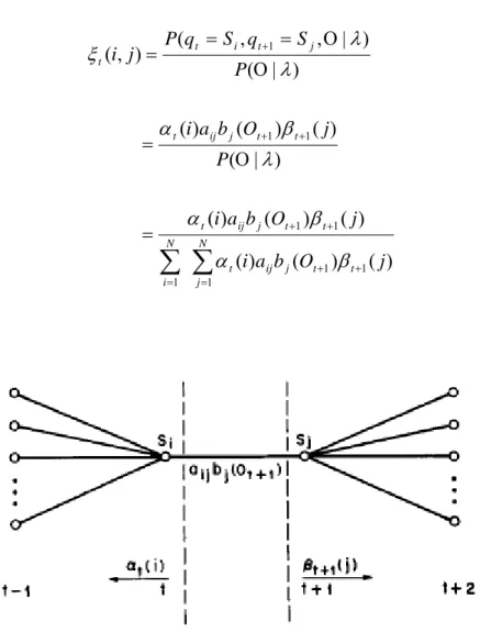
The training procedure adjusts the model parameters (A, B, π) to maximize the probability of generating the training sequenceΟ given the HMM modelλ. We solve this problem with an iterative procedure, known as Baum-Welch method. We begin by defining a variableξt(i,j), the probability of being in state Si at time t, and state Sj at time t+1 given the

model and the observation sequence:

) , | , ( ) , ( 1 λ ξt i j =P qt =Si qt₊ =Sj Ο .

Figure 3-6 illustrates the conditions required by the variable. Clearly, ξt(i,j) can be

rewritten involving the forward and backward variables in the form

∑

∑

= + + = + + + + + = Ο = Ο Ο = = = N j t t j ij t N i t t j ij t t t j ij t j t i t t j O b a i j O b a i P j O b a i P S q S q P j i 1 1 1 1 1 1 1 1 1 ) ( ) ( ) ( ) ( ) ( ) ( ) | ( ) ( ) ( ) ( ) | ( ) | , , ( ) , ( β α β α λ β α λ λ ξ

Figure 3-6 Illustration of sequence of operations required for the computation of the joint event that the system is in state Si at time t and state Sj at time t+1 [12]

Then, we define the variableγt(i), which represents the probability of being in state Si at

time t, given the observation sequence Ο and the model λ: ) , | ( ) ( λ γ_t i =P q_t =S_i Ο .

γt can also be expressed in terms of the forward-backward variables,

∑

= = Ο = _N i t t t t t t t i i i i P i i i 1 ) ( ) ( ) ( ) ( ) | ( ) ( ) ( ) ( β α β α λ β α γ .

In addition, we can relateγt(i) toξt(i,j) by summing over j, giving

∑

= = N j t t i i j 1 ) , ( ) ( ξ γ .

Therefore, the sum ofγt(i) over time may be interpreted as the expected number of times

that state Si is visited, or equivalently, the expected number of transitions made from state Si. That is i 1 1 S from ns transitio of number expected (i) =

∑

− = T t t γ .

Similarly, the sum ofξt(i,j) over time may be interpreted as the expected number of

transitions from state Si to Sj. That is

j i 1 1 S to S from ns transitio of number expected j) (i, =

∑

− = T t t ξ .

Using the above formulas, we can iteratively reestimate the model parameters of a HMM by simply “counting events.” The reestimation formulas forπ,A, B are

) ( 1) (t at time S state in times of number expected _{i 1} i i γ π = = =

∑

∑

− = − = = = ₁ 1 1 1 i j i (i) j) (i, S from ns transitio of number expected S to S from ns transitio of number expected _T t t T t t ij a γ ξ

∑

∑

= = = = = _T t t T v o t s t t k j k t v k b 1 . .1 j j (j) (j) S state in times of number expected symbol observing and S state in times of number expected ) ( γ γ

The reestimated model is denoted as λ=(A,B,π), and it has been proven that the reestimation procedure increases the likelihood of the model generating the observation sequence, i.e., P(Ο|λ)>P(Ο|λ).

3.5 Layered HMM

A layered HMM (LHMM) is the extension of standard HMM [15], developed to decompose the parameter space in a way that could enhance the robustness of the system by reducing training and tuning requirements. A problem is hierarchically divided into sub-problems with smaller scope, and the final solution is obtained by merging the results of the sub-problems.

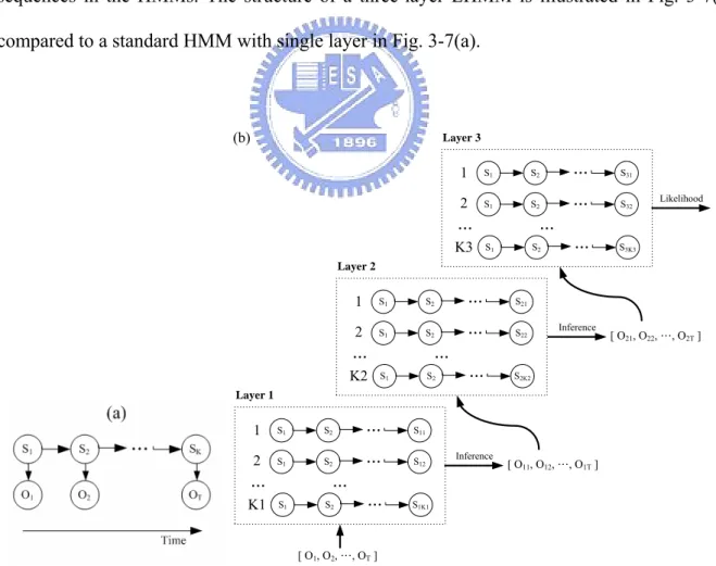
In LHMMs, each layer is connected to the next layer via its inferential results. The representation segments a problem into distinct layers that operate at different temporal granularities, which correspond to the window sizes or vector lengths of the observation sequences in the HMMs. The structure of a three-layer LHMM is illustrated in Fig. 3-7(b) compared to a standard HMM with single layer in Fig. 3-7(a).

S1 S2 ... S11 S1 S2 ... S12 S1 S2 ... S1K1 1 2 K1 ... ... Layer 1 S1 S2 ... S21 S1 S2 ... S22 S1 S2 ... S2K2 1 2 K2 ... ... Layer 2 S1 S2 ... S31 S1 S2 ... S32 S1 S2 ... S3K3 1 2 K3 ... ... Layer 3 [ O1, O2, …, OT] [ O11, O12, …, O1T] Inference [ O21, O22, …, O2T] Inference Likelihood (b)

Figure 3-7 Graphical representation of (a) a standard HMM (b) an architecture of three-layer LHMM

There are two approaches to performing inference with LHMMs [15]: maxbelief and distributional approach. In the maxbelief approach, the model with the highest likelihood is selected and provided as an input to the HMMs at the next level. In the distributional approach, the full probability distribution over the HMMs in the lower level is passed to the next-level HMMs.

Since the training and learning of each layer of LHMM is performed individually, LHMM successfully avoids the drawback of standard HMM – an excess of parameters and over-fitting of limited training data. At the same time, it preserves the advantage of HMM being robust to changes in the segmentation of observations. In addition, it suits the type of problems with layered structures.

Chapter 4

Proposed Action Recognition Scheme

In this chapter, we present our action recognition mechanism that aims to detect actions of an upper human body. Section 4.1 first introduces the system framework. The following sections detail the procedures of the system. Section 4.2 defines the features we employ and the algorithm of feature extraction. In Section 4.3, features are transformed to pose symbols. Section 4.3 depicts the actions to be recognized and the recognition scheme.

4.1 System Overview

The system framework consists of feature extraction, pose estimation, and action recognition as shown in Figure 4-1. First, we segment the human as foreground object from an image and then extract local and global features from the segmentation result. Second, the human pose is estimated by two separate arm pose estimators using extracted features. After processing each frame, the human action is recognized by using sequences of arm poses and the global feature based on layered hidden Markov models (LHMMs).

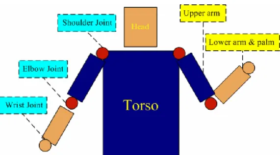
In this thesis, a human is modeled as a collection of body parts [8] as Figure 4-2, including head, torso, upper arms, and lower arms. Human segmentation is regarded as a part-based searching procedure. The local feature is composed of location information of each body part, and the global feature is made up of location relation of body parts. After obtaining the feature vectors in each frame, the high-level knowledge of human action can be inferred subsequently.

Figure 4-1 System Overview

In most cases, two arms’ interaction determines the action of an upper human body, so the recognition procedure focuses on arms without considering other parts. Furthermore, our strategy is to recognize two arms separately. The fundamental idea is that, by defining an adequate set of arm actions, we can decompose the human action recognition problem into two levels. In the first level, actions of two arms are recognized individually. In the second level, the combination of two arms is recognized as the human action. However, so far what we have is a large amount of feature vectors containing numerical location information of body parts which can not be directly perceived through the senses. Before starting the recognition procedure, we should translate confusing local feature vectors to simple but expressive symbols representing two arm poses.

After revealing the location of body parts, the joints between body parts are inferred. An arm pose is represented as a type of interrelationship of arm joints, including the shoulder, the elbow, and the wrist. For example, if one’s hand is raised, the wrist is above the shoulder and so is the elbow. The elbow is below the wrist at the same time. The method we adopt to estimate the arm pose is efficient and effective. All the defined pose symbols are listed in section 4.3.

Our recognition framework is based on the extension of hidden Markov models (HMMs). The HMM is a popular statistical tool for modeling time series data, and has been successfully used for numerous sequence recognition tasks, such as speech recognition. Modeling human actions to HMMs involves two procedures: training and recognition. The training procedure optimizes the parameters of HMMs. Each HMM is trained to represents a specific pattern. The recognition is achieved by finding the HMM with the maximum probability of generating the tested observation sequence. The difference of layered HMM (LHMM) from traditional HMM is the Markov models are structured as various layers for patterns with distinct scopes and the recognition results from the lower layer provide the input of the higher layer.

We present a two-layer HMM framework for human action recognition to meet the demand of our strategy of decomposing the human action recognition problem into two levels, arm movements and human actions. The goal of the lower layer is to recognize the actions of two arms individually using extracted features. The recognition result is regarded as the input of higher layer, which models the interaction of two arms. The local HMM and the global HMM in Figure 4-1 are in the lower layer, and the interaction HMM is in the higher layer.

Compared with a single-layer HMM structure, the layered approach has the following benefits, some of which were previously pointed out by [16].

1) A single-layer HMM is designed to train models on a large observation space, which might face the problem of over-fitting with limited training data. In contrast, the dimensions of the features we adopt in the layered HMM are smaller, resulting in more stable performance.

2) The models of the Local-HMM are reusable. In some cases, there is only one arm (right or left) dominating the action – raising one’s hand for example, so that the trained model for right arm can be transformed as left arm’s model in view of symmetry of human structures, and vice versa.

3) The Interaction-HMMs are less sensitive to slight changes in the low-level features because their observations are the output of the previous action recognizers, which are well trained to tolerate human segmentation flaws.

4) The two layers are trained independently so that it is easier to interpret and to enhance each layer. There are various types of HMMs, such as ergodic and left-right model. We can choose the most suitable type for each model in each layer individually instead of remaining a consistent type for all models.

5) The framework is general and extensible to recognize new human actions defined in the future.

4.2 Feature Extraction

4.2.1 Local Feature Definition

A human body can be modeled as a collection of body parts linked in a kinematic structure. It is natural to express such a model as an undirected graph with vertices representing parts and edges representing connections between parts. Since every part is connected and the connections between parts is acyclic, a human model fits the tree structure more specifically. The center part of body, head-torso, can be viewed as the root followed by children parts. Then, breadth first search order can be applied to our part detection scheme to find the locations of all parts hierarchically. The location information, which specifies a position, orientation and an amount of foreshortening of each part, forms the local feature. We record the scale of the length of the extracted arm and the standard model, since the length of an arm can vary due to foreshortening.

As shown in Figure 4-2, our model for a front-facing upper body has five “parts” or “combination of parts”: (a) head and torso, (b) two parts for upper arms, and (c) two parts for lower arms and palms. Two parts are linked by joints, shoulder joints and elbow joints. The wrist joints are the linkers of lower arms and palms. The head-torso part is defined as the “salient part” since it dominates the human body and it is easy to detect. On the other hand, the remains are categorized as “rest parts”. In this thesis, we assume users’ lower arms are exposed to simplify the human model. The assumption is fairly valid whether the users wear short sleeve shirts or roll up long sleeves. Consequently, the skin model for head and lower arms are the same and the clothing model for torso and upper arms are identical.

each vector comoponent specifies the location information of the part specified by the suffix. The posterior probability of a location vector L given an image I is formulated as,

i l ) ( }) { | ( ) | ( ) | ( ) | ( ) | ( ) ( ) | ( I p l I p l l p l l p l l p l l p l p I L

p = HT RUA HT LUA HT RLA RUA LLA LUA i

∏

∏

∝ i i i i parent i l p I l l p( | ₍₎) ( | ).

The above formulation, proved in [8], is a standard approximation adopted by many researches in the past. Generally, the prior probability is uniform distribution over all possible locations as long as the kinematic restriction is retained, which says that the head can be any position of the image and the left lower arm can be left-bottom or right-top of the left upper arm only if they are linked. Since detection in each frame is performed without prior knowledge from previous frames, it is reasonable to assume that all poses are equally possible. Furthermore, the detection of individual body parts through template matching is independent of each other. Hence, the likelihood of seeing an image given that the human is at some location can be modeled as the product of individual part likelihoods,

) | (li lparent(i) p

∏

∝ i i i p I l l I p( |{ }) ( | ).

The individual part likelihood is approximated as the ratio of foreground pixels inside a part to total pixels inside a part,

i i i l inside pixels total l inside pixels foreground l I p( | )= .

4.2.2 Local Feature Extraction

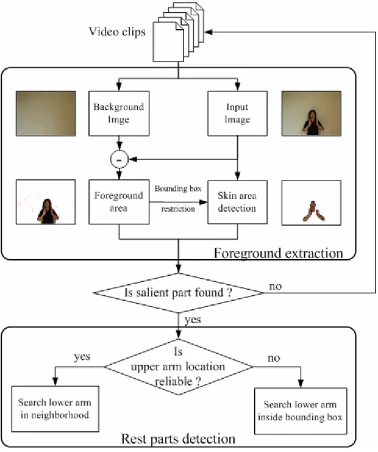
The algorithm of local feature extraction consists of two stages, foreground extraction and hierarchical part detection. The first stage extracts foreground area and skin area of an input image and meantime estimates the bounding box of foreground pixels. The second stage detects the location of each body part hierarchically from the salient part to rest parts. The algorithm is displayed in Figure 4-3.

First, the input image and background image are transformed to YUV color space. Background subtraction is performed on the Y component of the color values of the transformed pixels. The bounding box of the foreground area is then estimated to speed the detection of skin areas and body parts. Skin areas are detected by comparing the transformed color values to a human skin model [19]. We employ the chrominance components of YCbCr color model to eliminate the influence of luminance. By the end of this stage, we attain foreground plane and skin plane, where we further apply morphological operations to filter noise and enhance the completion of extracted foreground objects. The following parts detection procedure is searched on these planes.

The matching of body parts to prior models is searched at coarse grid locations instead of at pixel level. Although head and torso is viewed as a combination part, we have two detectors for head and torso doing different follow-up procedures. To start from the torso, the template of the torso is moved on the foreground plane to find the location with the highest probability. Since it is assumed that the color distributions of the torso and upper arms are the same, we learn the appearance model of clothing by building the YCbCr color histograms for rest parts detection. Head is searched on the skin plane in the area adjacent to torso. If head is found, we continue searching the rest parts, or else we simply drop the input video frame based on the assumption that human face must be seen to insure the existence of human being in the current image.

As the location of torso and the appearance model of clothing are collected, upper arms are detected and the reliability of the arm location is evaluated by the probability of the template matching. The higher probability implies the higher reliability of the arm location. If the location of upper arm is assured, lower arm is searched in the neighborhood. Otherwise, it is searched inside the bounding box.

4.2.3 Global Feature

In opposition to local feature specifying the information about parts themselves, the global feature defines the relation between parts. In our method, we record the distance relation between right and left palms. The distance relation is simply determined as near or far, instead of retaining measured numerical values. The classification is based on an adaptive threshold, which is proportional to the width of torso model. Hence, after detecting the locations of lower-arm-and-palm parts from local feature extraction algorithm, we can calculate the Euler distance of two palms and judge their distance relation without extra effort.

4.3 Pose Estimation

So far we obtain the abstract features of a human pose revealing where the body parts are, but the pose understanding remains unsolved. In this section, we propose an efficient and effective method to interpret a pose in a naïve way. Instead of building a representative codebook from training data and matching extracted features to all the pose exemplars in the codebook as adopted in the exemplar-based methods [4, 5, 7, 8], our proposed rule-based method estimates a pose according to the relation of joints.

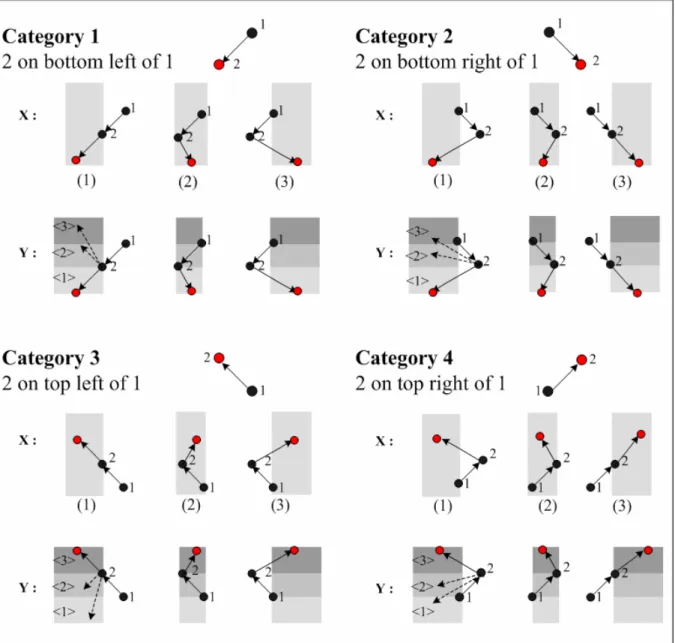
All the defined patterns for either right arm or left arm poses are listed in Figure 4-4. The circles represent joints, including the shoulder, the elbow, and the wrist labeled from one to three respectively. We can organize them in terms of the following taxonomy. Patterns are first grouped into four categories according to the relative position of joint 2 (elbow) and joint 1 (shoulder). The category one stands for the cases that joint 2 is on bottom left of joint 1. The category two stands for the cases that joint 2 is on bottom right of joint 1, and the category

three and four similarly stand for the cases that joint 2 is on top left and top right of joint 1 respectively.

Figure 4-4 Pose estimation from joints relation. The circles represent joints, including the shoulder, the elbow, and the wrist labeled from one to three respectively.

Each of the categories is then divided into smaller groups based on the x and y coordinate. Take x coordinate into consideration first. All the patterns in the same category are split into three partitions depending on whether the x coordinate of joint 3 (wrist) is left to,

between, or right to the coordinates of joint 1 and joint 2. Then, each partition is further split into three sub-partitions depending on whether the y coordinate of joint 3 is below, between, or above the coordinates of joint 1 and joint 2.

Consequently, each time the location information of parts is achieved, the coordinates of joints are used to estimate the pose by deciding which category, partition, and sub-partition the pose belongs to. Each pattern of pose is assigned a three digit codeword. The first digit indicates the category the pattern belongs to, and the second and third digits specify the partition and the sub-partition.

There is one point deserved mentioning that the patterns on the left side of Figure 4-4 are symmetric to those on the right side. Due to this symmetric property, the advantage of reusability of trained HMMs, showed in section 4.1, is easy to implement. All we need to do is to transform the trained HMMs of one arm to symmetric HMMs, which are sufficient to represent the other arm’s trained models.

4.4 Action Recognition

4.4.1 Framework overview

We present a two-layer HMM framework for human action recognition to meet the demand of our strategy to decompose the human action recognition problem into two levels, arm actions and human actions. As the Figure 4-5 shows, the local HMMs and the global HMM are in the lower layer, responsible for the recognition of arm actions using sequences of estimated arm poses and extracted global features. The two local HMM recognizers represent right and left arm respectively. The recognition results of all recognizers are transformed into feature vectors and regarded as the input of higher layer, which models the interaction of two arms and output the final recognition result of the human action.

The HMM recognizers take charge of the evaluation process. Given a model and a sequence of observations, we need to compute the probability that the observed sequence was produced by the model. We can also view the evaluation process as one of scoring how well a given model matches a given observation sequence. In other words, if we try to choose among several competing models, the solution to the evaluation process allows us to choose the model which best matches the observations.

There are two approaches to performing inference with LHMMs: maxbelief and distributional approach. In the maxbelief approach, the model with the highest likelihood is selected and provided as an input to the HMMs at the next level. In the distributional approach, the full probability distribution over the models is passed to the next-level HMMs. In this thesis, we propagate the maxbelief of the lower layer as the observation of the higher layer. However, we also pass the probability distribution to provide detailed recognition results.

Local-HMM 1 Action-HMM 1 Action-HMM 2 . . . Local-HMM 2 Action-HMM 1 Action-HMM 2 . . . Global-HMM Relation-HMM 1 Relation-HMM 2 . . . Lower Layer Higher Layer Interaction-HMM Interaction-HMM 1 Interaction-HMM 2 . . . Preprocessing Video clips Right Arm

Posture Features Posture FeaturesLeft Arm

Global Relationship Feature ] , , , [Ο'1 Ο'2 L Ο'T1 Recognition Result Inference

Figure 4-5 The two-layer HMM framework.

There are two approaches to performing inference with LHMMs: maxbelief and distributional approach. In the maxbelief approach, the model with the highest likelihood is selected and provided as an input to the HMMs at the next level. In the distributional approach, the full probability distribution over the models is passed to the next-level HMMs. In this thesis, we propagate the maxbelief of the lower layer as the observation of the higher layer. However, we also pass the probability distribution to provide detailed recognition results.

4.4.2 Action Definition

The list of local and global actions for one arm is defined in Table 1. There are four types of local actions to describe one’s arm, including raising, waving, clapping, and still. Generally speaking, one man’s arms are hung down naturally toward the ground while standing doing nothing. The status of one arm is named “still”. The action of the “raising” is initialized from the pose of “still”. The participant raises his arm gradually until the hand is overhead. The “waving” action is to swing one’s arm overhead left and right alternately. While one man clapping his hands in front of his chest, his arms appear to strike the air continuously, and such movement is the means to perceive the action “clapping”.

Local action description

Raising one arm raised overhead

Waving one arm swinging overhead left and right alternately Clapping one arm continuously striking the air in front of the chest

Still one arm hung down naturally

Global action description

Near-Far the distance of two hands being near and far alternately Far the distance of two hands remaining far all the time

Table 1 Description of local and global actions

Since a human being has two hands, it is reasonable for one man to raise any of his hands while he receives the instruction to raise his hand. Therefore, the “raising” action is further divided into “raising one’s right hand” and “raising one’s left hand”. In a similar way, the “waving” action and the “still” action are divided into actions for left and right hands. Consequently, the number of local action types we can recognize is seven instead of four.

On the other hand, the global actions used to describe the distance relation of two hands are simply defined as two types of “Near-Far” and “Far” because all the human actions we

can recognize fall into these two categories. The “Near-Far” action stands for the case that the distance of two hands is near and far alternately. The “Far” action stands for the case that two hands are always far from each other.

The logical relations between human actions, local actions, and global actions are summarized in Table 2. The human actions can been seen as combinations of local actions of two arms and global actions of two hands. Note that we define a new action “stretching” of human actions different from those of local actions pointed out in Table 1. The “stretching” action is an ensemble of two arms raised and the global action labeled as far. The only difference between “raising” and “stretching” is the number of raised arms, which is one and two respectively. The “raising” action covers the cases whether one raises his right arm or left arm as long as the other arm remains still. In a similar way, the “waving” action is an ensemble of one arm waving, the other arm being still, and the global action being far. Since the “clapping” action stands for one clapping his both hands, it is reasonable that the global action is Near-Far with one’s hands joining together and separating alternately.

Human actions Local actions Global actions

Raising One arm is raised, and the other arm is still. Far

Stretching Two arms are raised. Far

Waving One arm is waving, and the other arm is still. Far

Clapping Two arms are doing clapping. Near-Far

4.4.3 Lower-Level HMM

The fundamental idea of the HMM recognizer is to construct a model for each of the actions to be recognized. The elements of a HMM model are states and three probability distributions, including state transition distribution, observation emission distribution, and state initial distribution. The common notation for a model is λ, and the symbol for the probability of an observation sequence Ο given the model isP(Ο|λ).

There are numerous types of HMMs, varying in state transition constraints. In this thesis, we adopt two distinct structures – the ergodic model and the left-right model as shown in Figure 4-6. An ergodic model, or fully connected HMMs, has the property that every state of the model can be reached from every other state. A left-right model [12], also called Bakis model, has the property that as time increases the state index increases (or stay the same), i.e., the states proceed from left to right. Clearly, the left-right type of HMM can better models signals whose properties change over time – e.g., speech, than the ergodic model. In the same manner, the left-right model can be used for non-cyclic motions such as arm-raising, while ergodic model can be used for periodic motions such as hand-clapping.

Figure 4-6 Illustration of distinct types of HMMS. (a) A 3-state ergodic model. (b) A 3-state left-right model.

To summarize, each of the four cases of local actions and two cases of global actions has a corresponding model, well-trained to represent the movement. For cyclic motions – “Waving”, “Clapping”, “Near-Far”, we select the structure of ergodic model. On the contrary, we use left-right model for the rest.

After constructing and training each action model of HMM recognizers, the probability of each model generating the observation sequence to be recognized is evaluated. We combine the maxbelief output of all recognizers as an observation to the higher layer. The new observation is propagated to the next layer along with the detailed probability distribution over all models.

4.4.4 Higher-Level HMM

In this layer, the recognition process of the human action is based on the combinational patterns of the three lower-level HMM recognizers, namely the observation sequence. The new observation symbol is a high-dimensional feature vector, i.e., also a Boolean vector, which very likely results in over-fitting to limited training data. Briefly, the training of the observation emission probability distribution of a HMM is to count the appearing times of each observation in training data. In the case of high-dimensional discrete observations, a large proportion of observations do not occur in the training data. Thus, the emission probabilities of these unseen observations are equally low for all action models. Therefore, recognizing an unseen observation sequence may lead to failure even the unseen observation sequence is similar to some observation sequence which has appeared before.

To solve the problem, we propose a modified method of generating the observation emission probability distribution. The emission probability of each observation symbol is

applied a weighting. The weighting favors two types of defined observation symbols. The first type is the observation with smaller hamming distance to the input symbol. We compute the distance between the input symbol and the considering defined symbol, and the smaller distance implies the higher weighting applied to the considering defined symbol. The second type is the observation with higher max belief. We summation the probabilities, propagated along with the observation, of the models with maxbelief, and the higher summation implies the higher weighting. To formulate the weighting, the following notations are first defined. D = the number of HMMs in the Lower-Level

N = the number of HMMs in the Higher-Level

)

,...,

(

}

,...,

{

)

,...,

(

)

,...,

(

1 1 1 ' 1 ' ' nD n n N D D

s

s

S

S

S

S

p

p

P

o

o

O

=

=

=

=

:input observation vector

vel e Lower-Le HMMs in th over all stribution ability di input prob : Level he HMMs in t set of all servation defined ob : evel e Higher-L HMMs in th vector of servation defined ob :

The weighting is formulated as

∑

=

×

=

1

)'

,

(

tance

HammingDis

_normalized

10

-nd

s

p

O

S

d n n

W

The normalization adjusts the probability summations of all action models to values between 0 and 1.

We demonstrate the influence of applying the weighting by an example. Assume an observation sequence containing only one observation is propagated from the lower layer along with the probability distribution. The input observation is denoted as O’ in the following Table 3. There are three trained action models: Waving, Raising, and Stretching. Any of these three models has only one observation appearing in training data, denoted as S1, S2, and S3 individually. Hence, other “unseen” symbols for the model have equally low emission

probabilities. The input observation O’ happens to be an “unseen” symbol for the three models. Thus, the likelihood of the three models generating O’ is equally low based on the traditional observation emission probability distribution, and the recognition result might fail. However, if we apply the weighting to the emission probability distribution, as we can see, the weighting favors the “Waving” action. The input observation sequence is recognized as “Waving”, which is the correct result. The probability P(O’ | λ) differs among the three models, meaning the discriminability of the modified LHMM improves.

P -62 -15 -221 -221 -45 -221 -126 -71 -41 0 Input

Observation

O’ 0 1 0 0 1 0 0 0 0 1

Hamming

Distance Sum P Normalized P Weight

Waving Symbol S1 0 1 0 0 0 0 0 1 0 1 2 (-15)+(-71)+0 = -86 0.74 10-2 x 0.74 Raising Symbol S2 1 0 0 0 0 0 0 1 0 1 4 (-62)+(-71)+0 = -133 0.59 10-4 x 0.59 Stretching Symbol S3 1 0 0 0 1 0 0 0 0 1 2 (-62)+(-45)+0 = -107 0.67 10-2 x 0.67

Chapter 5

Experimental Results and Discussion

We have implemented the human action recognition system based on our proposed method and have tested the system performance on real human action videos. The system is capable of recognizing six distinct actions, including “Raising the right arm”, “Raising the left arm”, “Stretching”, “Waving the right arm”, “Waving the left arm”, and “Clapping”. The video content was captured by a digital camera (NTSC, 30 frames / second) with the pixel resolution of 320x240. For simplicity, the background of each video clip is assumed static and uniform in order to facilitate human segmentation. Each video clip is sampled every three frames to reduce temporal redundancy. The duration of the sampled clips is from 14 to 62 frames, in which an action can be recognized whether the movements are fast or slow.

All data is separated into two sets, the training data set and the testing data set. Training set contains 1 person wearing different clothes repeatedly doing four types of actions — “Raising the right arm”, “Stretching”, “Waving the right arm”, and “Clapping”. Figure 5-1 shows some example video clips of the training data. Note that the training set excludes on purpose the training samples of the two actions of “Raising the left arm” and “Waving the left arm” because the trained models of the symmetric actions of the two actions can be reused and transformed into the desired models directly.

Testing set contains 7 persons doing all the defined actions. Each action is repeated three times in average. Recognizing this testing set successfully reveals that the action models trained from a restricted data set provide sufficient discrimination to recognize movements with slight difference from the defined actions.

Figure 5-1 Example clips of each human action in training data set

The action recognition task is started by human segmentation. The three human parts of (a) head and torso, (b) two parts for upper arms, and (c) two parts for lower arms and palms are segmented out, and the amounts of translation, rotation, and scaling of each body part are assembled to local and global features. The extracted local features are further used for arm pose estimation. Figure 5-2 shows the examples of human segmentation results of training video clips. Colored rectangles represent human body parts. Shoulder joints and elbow joints are connected in red color; elbow joints and wrist joints are connected in yellow. The relation of the three joints is encoded to a pose symbol according to Figure 4-4.

After processing feature extraction and pose estimation of every frame of a video clip, each HMM recognizer in the lower level collects the sequence of observations and all the trained action models inside the recognizer compute the probability of generating the corresponding observation sequence Oi. Then, the model with the highest likelihood inside each recognizer is selected, and the selection results of all recognizers is combined to a feature vector as an input to the HMMs in the higher level along with the original probability distribution. We regard the input sequence for the HMMs in the higher level as a new observation sequence O’ in contrast to the input sequence for the HMMs in the lower level Oi. In the same manner, the trained action models compute the probability of generating the new observation sequence O’. The video clip is recognized as the action with the max probability. The example of complete recognition process is shown in Figure 5-3.

(a) Raising (right arm)

(b) Stretching

(c) Waving (right arm)

(d) Clapping

Right arm sequence: 131 131 131 131 121 121 111 111 111 111 111 111 111 111 113 113 313 313 313 313 313 313 313 313 313 313 313 313 313 313 313 313 323 323 323 323 323 323 323 323 323 323 323 323 333 333 333 333 333 333 333 333 333 333 333 333 333 333 333 333 333 333

Left arm sequence: 231 231 231 231 231 231 231 231 231 231 231 231 231 231 231 231 232 232 233 233 433 433 433 433 433 433 433 433 433 433 433 433 433 433 433 433 433 433 433 433 433 433 433 433 433 433 433 433 433 433 433 433 433 433 433 433 433 433 433 433 433 433 Feature Extraction Log( P( Or| Raise) ) = -135.93 Log( P( Or| Wave) ) = -127.55 Log( P( Or| Clap) ) = -407.45 Log( P( Or| Still) ) = -339.85 Log( P( Ol| Raise) ) = -107.49 Log( P( Ol| Wave) ) = -151.24 Log( P( Ol| Clap) ) = -359.20 Log( P( Ol| Still) ) = -319.40 Log( P( Og| Near-Far) ) = -80.39 Log( P( Og| Far) ) = 0.00

P( O＇| Raising-right ) = 0.00008 P( O＇| Raising-left ) = 0.00847 P( O＇| Waving-right ) = 0.00848 P( O＇| Waving-left ) = 0.00008 P( O＇| Stretching ) = 0.00917 P( O＇| Clapping ) = 0.00000

Stretching Clip

Local recognizer of right arm Local recognizer of left arm Global recognizer

Recognition result: Stretching

0100 1000 01

O

= <

>

Interaction

HMM

Global Features Local Features Defined Poses

Pose Estimation

We compare the recognition results of 1-layered HMM (traditional HMM), 2-layered HMM with trained emission distribution, and our proposed 2-layered HMM with weighted emission distribution. The results are summarized in the following tables. Table 4 demonstrates the correct recognition numbers and rates of the three distinct systems. Table 5 shows the confusion matrix.

raise stretch wave clap sum precision

number of testing clips _right (24) left (6) (27) right (24) left (9) (21) (111) 1-layered HMM 21 1 27 21 3 21 94 84.68% 2-layered HMM

with trained emission distribution 24 6 27 20 6 21 104 93.69% 2-layered HMM

with weighted emission distribution 24 6 27 21 6 21 105 94.59% Table 4 Precision of the three distinct systems

Overall, the more complex system implies the higher precision. Our proposed system presents the best result and reaches the precision of 94.59%. However, the confusions between waving and raising are caused by the abnormal movements of the acting person. The standard movement of the waving action is to swing one’s arm overhead left and right alternately as shown in Fig. 5-4(a), and the movement of the failed clip obviously disobeys the rule from the segmentation result shown in Fig. 5-4(b). As it happens, the sequence of the abnormal waving poses is part of the raising action. Therefore, the abnormal waving clips are recognized as the raising action.

Confusion matrix for 1-layered HMM

Raising (right hand)

Raising

(left hand) Stretching

Waving (right hand)

Waving

(left hand) Clapping

Raising (right hand) 21 3

Raising (left hand) 2 1 3

Stretching 27

Waving (right hand) 3 21

Waving (left hand) 6 3

Clapping 21

Confusion matrix for 2-layered HMM with trained emission distribution

Raising (right hand)

Raising

(left hand) Stretching

Waving (right hand)

Waving

(left hand) Clapping Raising (right hand) 24

Raising (left hand) 6

Stretching 27

Waving (right hand) 4 20

Waving (left hand) 3 6

Clapping 21

Confusion matrix for 2-layered HMM with weighted emission distribution

Raising (right hand)

Raising

(left hand) Stretching

Waving (right hand)

Waving

(left hand) Clapping Raising (right hand) 24

Raising (left hand) 6

Stretching 27

Waving (right hand) 3 21

Waving (left hand) 3 6

Clapping 21

Table 5 Confusion matrix of the three distinct systems, 1-layered HMM, 2-layered HMM with trained emission distribution, and 2-layered HMM with weighted emission distribution.