串接式類神經網路在財務時間序列模型與預測之研究

行政院國家科學委員會專題研究計畫 成果報告

串接式類神經網路在財務時間序列模型與預測之研究

研究成果報告(精簡版)

計 畫 類 別 ： 個別型

計 畫 編 號 ： NSC 94-2416-H-151-005-

執 行 期 間 ： 94 年 08 月 01 日至 95 年 07 月 31 日

執 行 單 位 ： 國立高雄應用科技大學資訊管理系

計 畫 主 持 人 ： 柯博昌

計畫參與人員： 碩士班研究生-兼任助理：簡偉倫、黃慶俊、高怡君

處 理 方 式 ： 本計畫涉及專利或其他智慧財產權，2 年後可公開查詢

中 華 民 國 96 年 01 月 22 日

行政院國家科學委員會補助專題研究計畫

; 成 果 報 告

□期中進度報告

（計畫名稱）

串接式類神經網路在財務時間序列模型與預測之研究

計畫類別：

;

個別型計畫 □ 整合型計畫

計畫編號：NSC 94-2416-H-151 -005

執行期間：

2005 年 8 月 01 日至 2006 年 12 月 20 日

計畫主持人：柯博昌

共同主持人：

計畫參與人員：簡偉倫、高怡君、黃慶峻

成果報告類型(依經費核定清單規定繳交)：

;

精簡報告 □完整報告

本成果報告包括以下應繳交之附件：

□赴國外出差或研習心得報告一份

□赴大陸地區出差或研習心得報告一份

;

出席國際學術會議心得報告及發表之論文各一份

□國際合作研究計畫國外研究報告書一份

處理方式：除產學合作研究計畫、提升產業技術及人才培育研究計畫、

列管計畫及下列情形者外，得立即公開查詢

□涉及專利或其他智慧財產權，□一年

;

二年後可公開查詢

執行單位：國立高雄應用科技大學 資管系

中 華 民 國 95 年 12 月 20 日

串接式類神經網路在財務時間序列模型與預測之研究

摘

要

由於全球化競爭的結果，各國政府均必需正視國際金融變動對本國的經濟局勢影響，

而國際化企業的決策者面對未來金融局勢的波動，更需進一步掌握其發展趨勢與控管其風

險，以避免造成企業獲利的衝擊與影響，同時避免企業處於高風險的營運狀態。過去相關

的實證研究多採用時間序列的迴歸模型，如線性時間序列模型（AR、MA、ARMA 與 ARIMA

等）與自我迴歸條件變異模型（ARCH、GARCH 與 GARCH-M 等）。不過，最近研究發現

總體時間序列資料普遍為非定態(Non-stationary)，如果直接對原始財務資料進行迴歸分析，

將容易產生虛假迴歸(spurious regression)問題，並造成嚴重的估計誤差。雖然此一問題，可

針對個別變數進行差分以改善受時間趨勢影響的情況。但此一方法則存在著因使用差分後

資料可能會消除非定態時間序列間共整合關係(Co-integration Relationship)，以致喪失資料

長期的重要訊息。此外，目前新興的人工智慧技術，如

ANN、GA、GP、Fuzzy、Ant 與 PSO

等，均可以應用其非線性最佳化的搜尋能力，得到較佳的預測準確度，因此，本計劃將導

入一串接式的類神經網路模型，結合傳統時間序列模型與柔性計算的優點，應用類神經網

路模擬生物神經網路的特性，從真實複雜的金融財務資訊中獲取並累積經驗，儲存知識，

同時利用其智慧型的演算程序，重新組織並架構新的智慧型時間序列模型，進而提供更佳

的預測模型與風險控管機制

關鍵字：迴歸條件變異模型、類神經網路、選擇權、迴歸模型

Abstract

Global competition stimulates countries to confront the effects of international financial

changes to domestic economic environments. The decision-makers of global enterprises also face

future financial volatility, and further control the managing risk to avoid diminishing the profits

of business and increasing operating risk. The time series regression models, such as linear time

series analysis (AR, MA, ARMA and ARIMA) and Conditional Heteroscedastic Models (ARCH,

GARCH and GARCH-M), are widely used on the empirical researches in the past. But, the recent

researches find that the global time series financial data is non-stationary pervasively. It caused

series estimating error from spurious regression, if applying regressive analysis to raw financial

data directly. Although the spurious regression problem would be solved if differencing distinct

variables, it also causes eliminating co-integration relationship on non-stationary time series data

and fails to support a long-term equilibrium among them. Besides, the modem artificial

intelligent technologies, such as ANN, GA, GP, Fuzzy, Ant and PSO, achieve better predicting

accuracies based on their non-linear optimization capabilities. Therefore, we will introduce a

cascading neural network model in this project, which combines the advantages of conventional

time series models and soft computing technologies. By simulating the real bio-neural network,

our model accumulates experiences, stores necessary knowledge, computes smartly, re-organizes

more suitable time series modes intelligently, and provides better prediction models and risk

control mechanism finally, from real complex financial information database.

Keywords: GARCH、ANN、Options、Regression.

由於全球化競爭的結果，各金融市場的連動速度愈來愈快，此外各區域經濟體（如歐

盟等）的蓬勃發展，均宣示著未來國際金融版圖快速的移動與變化。此外，各式各樣新型

金融商品與衍生性金融商品的誕生，更呈現出未來金融商品的多樣性，而其相互間的連動

關係也將更趨於複雜。對政府而言，傳統的封閉保守財經政策，已無法符合未來的國際金

融局勢，各國政府均必需開放其金融市場，並正視國際金融變動對本國的經濟局勢影響。

另一方面，未來金融局勢（如外匯）的波動同樣也衝擊各國際化企業，各企業決策者除了

需面對金融局勢變動所造成的可能影響，如貨幣供給變化可能造成的利率變化外，更需要

進一步掌握其發展趨勢與控管其風險，以避免造成企業成本與獲利的衝擊，同時更可以避

免企業處於高風險的營運狀態，使企業營運風險增加。過去常用的相關實證研究多採用時

間序列的迴歸模型，如線性時間序列模型（AR、MA、ARMA 與 ARIMA 等）與自我迴歸

條件變異模型（ARCH、GARCH 與 GARCH-M 等）。不過，近代學者發現總體時間序列

資料普遍為非定態(Nostationary)，如果直接對原始財務資料進行迴歸分析，將容易產生虛

假 迴 歸(spurious regression) 問題，並造成嚴重的估計誤差。雖然此一問題，可採用

Box-Jenkins 方法對個別變數進行差分以改善受時間趨勢影響的情況。但此一方法則存在

著 因 使 用 差 分 後 資 料 可 能 會 消 除 非 定 態 時 間 序 列 間 共 整 合 關 係

(Cointegration

relationship)，以致喪失資料長期的重要訊息，並造成預測上的干擾與誤差。目前新興的人

工智慧技術，如

ANN、GA、GP、Fuzzy、Ant 與 PSO 等，均可以應用其非線性最佳化的

搜尋能力，得到較佳的預測準確度。

雖然目前許多人工智慧技術已被廣泛的用來預測投資組合績效或各類型的金融商品

價格，但面對各時間序列模型上計量方法的不斷改進與創新，其準確度也不斷的改進。所

以，本計劃將導入以串接式的類神經網路模型為基礎的財務時間序列模型，其可以同時結

合傳統時間序列模型與柔性計算的優點，應用類神經網路模擬生物神經網路的特性，從真

實複雜的金融財務資訊中獲取並累積經驗，儲存知識，同時利用其智慧型的演算程序，重

新組織並架構新的智慧型時間序列模型，並進而提供更佳的預測模型與風險控管機制。

目前，在加入

WTO 之後，我國金融業直接面對國外的競爭，由於國際金融環境的日

趨複雜與金融商品的多樣性，各金融商品之間的關係也相對的複雜與非結構性，另一方面

投資者面對跨國金融商品不易瞭解其報酬及風險的特質，也容易造成其血本無歸。再加上

近年來由於政府推動金融自由化，金融控股公司如雨後春筍紛紛成立，許多新金融商品也

陸續被開發。雖然傳統結構化的時間序列模型近幾年在計量方法上不斷的修正與創新，但

如能結合類神經網路在非線性最佳化的能力，重新模組化時間序列模型，使目前各種序列

迴歸模型，如線性時間序列模型（AR、MA、ARMA 與 ARIMA 等）與自我迴歸條件變異

模型（ARCH、GARCH 與 GARCH-M 等），均能應用類神經網路模擬生物神經網路的特

性，一定能更準確的預測未來的趨勢變化，進一步提供企業決策者更精確的資訊趨勢，以

控管並降低其營運風險。

2.文獻探討

本計畫主要在傳統的時間序列模型中，加入類神經網路的人工智慧技術，期望能普遍

改善各時間序列模型的準確度，並研究此一嶄新的智慧型時間序列模型在各種財務金融應

用的應用價值。因此相關人工智慧技術與時間序列模型在財經策略與財務工程議題(如選

擇權定價，外匯期貨等)的國內外重要文獻探討如下：

1.

時間序列模型在財經議題上的應用

傳統上，時間序列模型被廣泛的應用於各財經議題的預測上，例如：以總體經濟

面的觀點來探討和預測股市變動，並探究該國總體經濟和股票市場可能存在的關聯性

[1]-[2]；Joseph發現美國的總體經濟指標和財務股價指數間存有長期的均衡關係[3]。至

於實證研究方法上，傳統迴規歸分析法是常用的方法之一，不過，由於總體時間序列

資料普遍為非定態，若直接進行迴歸分析會因為虛假迴歸而造成嚴重的錯誤估計[4]。

因此，Granger and Engle提出共整合的估計方法－誤差修正模型(Error Correction

Models, ECM)以改善上述問題[5]，但由於其只能估計單一共整合向量，所以Johansen

另外提出以多變量模型(VAR)為基礎來改善，並利用最大概似法同時估計多個顯著的

共整合向量[6]。

2. 人工智慧技術在交易策略上的應用

近幾年，人工智慧技術被廣泛應用於分析財務市場資料以發掘股票交易策略，其

中尤以遺傳演算法與遺傳程式規劃最為常見，例如：以遺傳演算法為基礎考慮使用者

偏好輔助製定投資決策的研究模型，研究結果顯示，在考慮交易成本下其投資報酬率

可以打敗大盤[7]。應用遺傳演算法以技術指標最佳化出交易策略，研究對象是台積

電，測試期間 (1999) 的平均報酬率為 85.46% 優於買入持有的 62.5% [8]。同樣使用

遺傳演算法挑選以技術指標為基礎的交易策略，其研究對象是S&P500 指數股價走勢，

研究期間為

1928 年到 1995 年，研究結果顯示，考慮交易成本下，遺傳演算法的研究

模式打敗買入持有而獲得超額報酬[9]。此外，藉由遺傳程式規劃，也可以在歷史股價

中搜尋交易策略，以獲取超額報酬。 以台灣發行量股價指數與美國S&P500 股價指數

為研究對象，研究發現遺傳程式規劃為基礎的搜尋模式優於隨機漫步 (Random Walk)

理論近

50%，由此證明這兩指數具有弱式效率市場假說 (Weak-Form Efficient Market

Hypothesis)[10]。應用遺傳程式規劃分析日內股價交易資料，為單一個別股票選出交易

策略，其交易策略產生的間距或顆粒度是

1 分鐘內，以路透社提供的線上即時資訊為

研究樣本，其研究期間的投資報酬率優於買入持有策略[11]。以往投資人以經驗分析

技術指標，有研究應用模糊理論做股價技術分析的交易策略，即以歷史股價的技術指

標做為模糊邏輯的輸入變數，追蹤股價的趨勢做為股票買進賣出交易決策依據，智慧

型模糊式交易策略的實驗結果，其投資績效除優於S&P 500 指數報酬率外，亦具有超

額報酬[12]。也有應用模糊邏輯與類神經網路做股票交易策略系統，即藉由此系統能

在即時且複雜的股票市場中過濾與整合大量的資料提供投資人正確有效的資訊，幫助

製訂買進賣出的決策。實證結果顯示，結合模糊邏輯與類神經網路確實能獲得超額報

酬[13]。

3. 人工智慧於選擇權定價的應用

結合一種新的機率理論與模糊理論的歐式選擇權，歐式買權 (Call) 賣權 (Put)選

擇權定價問題充滿不確定因素，有研究以歐式選擇權 (Black-Scholes) 買賣雙方期望的

價格為考量因素以期望值法與模糊理論協助定價，即以買賣雙方期望價格計算其效用

函數，轉換為模糊數，處理選擇權定價的不確定，進而算出模糊定價。該研究證明此

模式可行性且具有避險能力[14]。以GP逼近股價指數選擇權與股價之間的關係 [15]，

Black-Scholes 歐式選擇權模式的參數做為GP的搜尋目標之一，並且以蒙地卡羅模擬法

輔 助 資 料 分 析 ， 當 資 料 呈 現

Jump-Diffusion 時 ， GP 找 到 的 規 則 其 績 效 優 於 純

Black-Scholes，另外，所需的資料量少以及速度快。應用GP於衍生性金融商品之避險

[16]，研究對象是 S&P 500 指數選擇權，試圖藉由GP找出歐式賣回選擇權定價模式，

即由GP找出五個參數的最佳化，進行算出定價。研究結果顯示，投資的勝率並不如預

期，原因可能是研究期間不夠長，GP模型相較於Trigueros [17] 的B-S模型，避險能力

有近

8 成的正確率。另有應用GP於日內指數期貨選擇權套利 [18]，其為即時線上套利

系統，最短能在

10 秒內做出套利決策。研究結果顯示，在測試期間共有 196 次套利訊

號，訊號的錯誤率為

0 次，平均獲利為 381 英磅，投資報酬率顯著。影響選擇權價格

的五個因素有即期資產價格、到期日、標的資產股價報酬波動度、無風險利率、屐約

價格。通常以Greeks 表示，用數值分析或敏感度分析衡量五個變數變動時，對選擇權

價格的影響，美式買回選擇權 Greeks (係數)，然而用這兩種方法分析這些係數是耗時

且較為封閉的解法。 除外，使用GP決定Vega等風險係數[19]，即藉助GP平行處理能

力，評估的係數與模型，其投資報酬率優於一般的數值分析方法。

4. 人工智慧於外匯期貨的應用

應用模糊類神經網路模型預測時間序列的外匯利率走勢，模糊系統歷史資料學習

模擬人類思考規則成為模糊規則，並建成知識庫，應用遺傳演算法最佳化模糊類神經

網路的參數。實驗結果顯示，可以改善正確率，並有效追蹤外匯利率的走勢 [20]。透

過遺傳程式規劃，找出美國中央銀行進場干預 (Intervention) 外匯利率的訊號 [21]，

試圖在交易中獲得超額報酬，文中的利用 Granger 因果檢定得出的假設是央行進行干

預後，必定會影響匯率的走勢，投資人即可從中獲利。研究結果顯示，利用遺傳程式

規劃預測出央行進場干預的訊號，以及考慮交易成本的因素下，並無法獲得超額報酬。

以遺傳程式規劃與

Reinforcement Learning做為技術分析的工具，協助搜尋日內

(Intraday) 外匯交易策略[22]，即在 15 分鐘內以常用的 8 項技術指標找出交易策略。

研究結果顯示，相較於 Markov-Chain 線性規劃法與簡易的經驗法則，在不考慮交易

成本的情形下，遺傳程式規劃與 Reinforment Learning模型可以獲得超額報酬，若考慮

交易成本，則無法獲得超額報酬。也有以遺傳程式規劃發掘高頻率 (High Frequency)

外匯市場的交易策略 [23]，該研究以遺傳程式規劃建構的交易策略，結合相關的領域

知識以限制語意在策略表達的完整性、對稱性，其主要目的是提高交易策略的可讀性，

但有其他研究 [24]出會降低投資績效。該研究結果顯示，在納入語意限制的情形並不

會影響投資報酬率，其原因歸功於適應函數有加入報酬率的風險調整因子。

3.研究方法

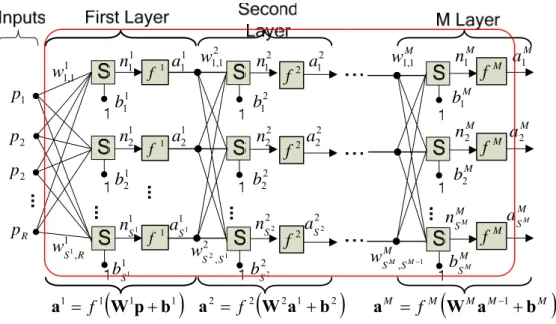
傳統的類神經網路架構圖如圖一所示，其中共有R個Inputs，M層的隱藏層(L

1

,

L

2

, …, L

M

)，第L

i

層具有S

i

個神經元，假設

p是Input Vector，W

i

是第i層的Weight Matrix，

b

i

是第i層的Bias Vector，a

i

是第i層隱藏層的Output Vector，則p、W

i

、

b

i

與

a

i

分別表示如

Equation (1)：

(1)

⎥

⎥

⎥

⎥

⎥

⎦

⎤

⎢

⎢

⎢

⎢

⎢

⎣

⎡

=

⎥

⎥

⎥

⎥

⎥

⎦

⎤

⎢

⎢

⎢

⎢

⎢

⎣

⎡

=

⎥

⎥

⎥

⎥

⎥

⎦

⎤

⎢

⎢

⎢

⎢

⎢

⎣

⎡

=

⎥

⎥

⎥

⎥

⎦

⎤

⎢

⎢

⎢

⎢

⎣

⎡

=

− − − i S i i i i S i i i i S S i S i S i S i i i S i i i R i i i i i i i i

a

a

a

a

b

b

b

b

w

w

w

w

w

w

w

w

w

W

p

p

p

p

M

M

L

M

M

M

M

L

L

M

2 1 2 1 , 2 , 1 , , 2 2 , 2 1 , 2 , 1 2 , 1 1 , 1 2 1 1 1 1

…

1 1 , 1

w

1

p

2

p

2

p

R

p

1 , 1_R S

w

1 1

b

1 2

b

1 1 S

b

…

1 f 1 f 1 f 2 1

b

2 2

b

2 2 S

b

…

2

f

2

f

2

f

…

2 1 , 1

w

2 , 1 2_S S

w

1 1

a

1 1

n

1 1 S

a

1 1 S

n

1 2

a

1 2

n

2 1

a

2 1

n

2 2 S

a

2 2 S

n

2 2

a

2 2

n

M

b

₁ M

b

₂ M SM

b

…

M

f

M

f

M

f

M

w

_1,1 M S SM M

w

_, −1 M

a

₁ M

n

₁ M SM

a

M SM

n

M

a

₂ M

n

₂

(

1 1

)

1 1

_W

_p

_b

a

= f

+

_a

2

_{= f}

2

(

_W

2

_a

1

₊

_b

2

)

M M

(

M M M

)

f

W

a

b

a

=

−1

+

圖

1. M-Layer Neural Network

假設f

i

(

⋅

)是第i層隱藏層的Activation Function，令p=a

0

, 則傳統類神經網路的操作

如Equation (2)。

(

1 1

)

for

0

1

2

1

1 1

, ...,

M-,

,

m

f

m m m m m+

=

+

_W

+

_a

+

_b

+

=

a

(2)

另 一 方 面 ， 傳 統 的 時 間 序 列 模 型 ， 如

AR(p) 、 ARMA(p,q) ， ARCH(p) 與

GARCH(p,q)，定義如 Equation (3)-(6)。

(3)

( )

_∑

= −

+

=

p i i t i t

r

r

p

AR

1 0

:

φ

φ

(4)

( )

_∑

_∑

= − = −

−

+

+

=

q i i t i t p i i t i t

r

a

a

r

q

p

ARMA

1 1 0

:

,

φ

φ

θ

(5)

( )

_∑

= −

+

=

=

p i i t i t t t t

a

a

p

ARCH

1 2 0 2

,

:

σ

ε

σ

α

α

(6)

( )

_∑

_∑

= − = −

+

+

=

=

q i i t i p i i t i t t t t

a

a

q

p

GARCH

1 2 1 2 0 2

,

:

,

σ

ε

σ

α

α

β

σ

其中φ

i,

θ

i

,

α

i

,

β

i

分別是一常數項，由於AR(p)、ARMA(p,q)的目標均在求解φ

i,

θ

i

的

值為何時，可使其誤差平方和達到最小，假設有N個觀察項r

p

, r

p+1

, r

p+2

,…, r

p+N-1

，以AR(p)

而言，定義Y, X,

Φ, E如下：

⎥

⎥

⎥

⎥

⎥

⎦

⎤

⎢

⎢

⎢

⎢

⎢

⎣

⎡

=

− + + 1 1 N p p p

r

r

r

Y

M

⎥

⎥

⎥

⎥

⎥

⎦

⎤

⎢

⎢

⎢

⎢

⎢

⎣

⎡

=

− − + − 1 2 1 0 1

1

1

1

N N p p p

r

r

r

r

r

r

X

L

M

M

M

M

L

L

⎥

⎥

⎥

⎥

⎥

⎦

⎤

⎢

⎢

⎢

⎢

⎢

⎣

⎡

=

Φ

p

φ

φ

φ

M

1 0

⎥

⎥

⎥

⎥

⎥

⎦

⎤

⎢

⎢

⎢

⎢

⎢

⎣

⎡

=

− + + 1 1 N p p p

E

ε

ε

ε

M

也就是說，Y = X⋅Φ + E，目標為minimize E

2

_，而

E

2

= (Y-X

⋅Φ

)

t

⋅

(Y-X

⋅Φ

)

0

2

=

Φ

∂

∂E

(

) (

)

[

]

0

2

=

Φ

⋅

−

Φ

⋅

−

Φ

∂

∂

=

Φ

∂

∂

X

Y

X

Y

E

t

(Y-X

⋅Φ

)

t

⋅

(Y-X

⋅Φ

)=(Y

t

-

Φ

t

⋅

X

t

)

⋅

(Y-X

⋅Φ

)

=Y

t

Y - Y

t

X

Φ

-

Φ

t

X

t

Y +

Φ

t

X

t

X

Φ

Because Y

t

Y is independent of B,

( )

=

0

Φ

∂

∂ Y

Y

t

.

[

]

( )

Y

X

X

X

X

X

Y

X

X

X

Y

X

X

Y

X

X

Y

X

X

Y

E

t t t t t t t t t t t t t

2

2

0

2

2

2

2

=

Φ

=

Φ

+

−

=

Φ

+

−

−

=

Φ

Φ

+

Φ

−

Φ

−

Φ

∂

∂

=

Φ

∂

∂

Finally,

Φ

= (X

t

X)

-1

X

t

Y

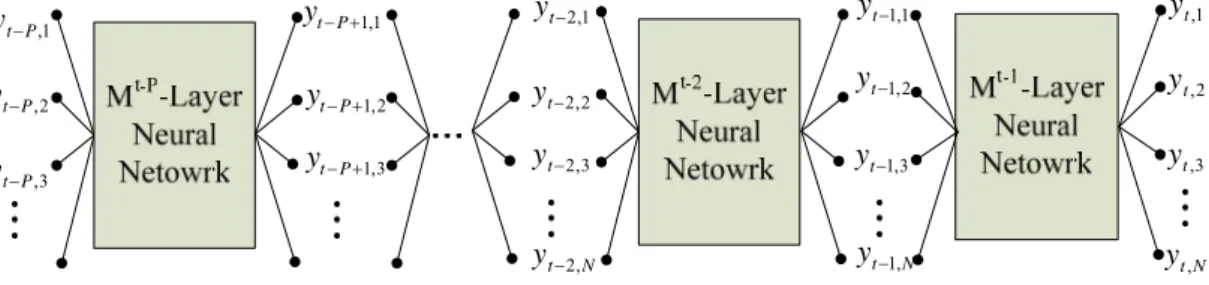
ARMA(p,q)與 AR(p)的解法類似，只要重新定義 X, Φ即可。結合上述類神經網路

模型與時間序列模型的優點，本計劃將提出一嶄新的串接式類神經網路模型，將原有

時間序列模型的線性參數組合，改以類神經網路取代之，希望藉由柔性計算的非線性

最佳化特性，進一歩改善其預測結果。

1 , t y 2 , t y 3 , t y N t y_, 1 , 1 − t y 2 , 1 − t y 3 , 1 − t y N t y−1, 1 , 2 − t y 2 , 2 − t y 3 , 2 − t y N t y−2, 1 , P t y− 2 , P t y₋ 3 , P t y− 1 , 1 + −P t y 2 , 1 + −P t y 3 , 1 + −P t y

圖

2. Cascading Neural Network Model

4. 實證結果與分析

本篇所使用的方法是以類神經迴歸係數模型以及

BS Model 的五個參數來實

作之，因此我們藉此導出的式子如下：

V

T

r

X

S

PV

=

β

₀

+

β

₁

*

+

β

₂

*

+

β

₃

*

+

β

₄

*

+

β

₅

*

(20)

其中每一個

β (i=0,1,2,3,4,5)分別代表著一個類神經網路，除了β

i 0以外，其它

五個類神經則是分別對應至BS Model的五個參數{ S, X ,r, T, V }，以求能藉此找

出一個評估選擇權價格的線性方程組，每個

β 所對應的參數資料如表三所示。

i 表三 βi

所輸入的參數資料

βi 輸入集合 β0 (X, T) β1 (X, T, S, V) β2 (X, T, S) β3 (X, T+1, T+2, T+3) β4 (X, T+1, T+2, T+3) β5 (X, T, ₋₁, , ) i t σ ₋₂ i t σ ₋₃ i t σ

而在這中間我們從

MySQL 資料庫內取出他的股票價格、履約價格以及執行

日期，到期日等四項資料，從中我們必需另外計算其到期日期至執行日期所包

含的天數，以及股價的波動率，在此波動率我們以取執行日期的前

30 天至執行

日期當作其樣本，以求能夠符合實際運算的價值，接著我們必需設定類神經的

參數如表四。

表四 類神經的參數設定

輸入層個數

4

隱藏層層數

2

輸出層個數

1

隱藏層個數

6

訓練週期

100

訓練樣本比率

0.8

測試樣本比率

0.2

學習率

0.1

激化函數

Sigmoid

網路模型

倒傳遞網路模型

三、績效評估

在此我們在表五以及表六分別列出NNC與BS Model的取絕對值delta避險的

誤差，所有的變動加總誤差值

ξNNC=200.56 和

ξBS=714，這些結果可以很顯然

的看出本篇所提出的NNC模型績效優於BS Model。

本篇所要達成的目標為能夠評量整個選擇權市場的公式，並希望能以此公

式來代替

BS Model，因其假設與現實有許多出入，並且藉由本篇所新創的公式—

類神經網路係數模型來尋找一組能計算其價值的係數值，因此在短期內首要目

的為能找出一組係數值能夠凌駕於

BS Model 在歐式選擇權方面的評價，但這組

係數值因其為類神經網路在非線性模型中求得的結果，因此其係數因隨著市場

的變動而做些微的調整。當然，由於歐式選擇權與美式選擇權有許多不同之處，

因此在未來我們不排除要新增一條專門為美式選擇權評價的係數模型，其中可

能要加以考慮的因素不外乎是可能交易的執行日期與利息發放等相關議題，

表五 Delta Hedge Error – NNC 模型 (Year: 2004) 執行 價格 三月 四月 五月 六月 九月 5300 NA NA NA 200.5 124.4 5500 NA NA NA 289.2 188.3 5700 NA NA NA 198.5 167.6 5900 NA NA NA 295.6 127.1

6100 NA NA NA 187.7 170.9 6200 NA 288.3 NA NA NA 6300 NA 264.6 0.0 125.0 160.1 6400 NA 404.5 211.0 NA NA 6500 NA NA 219.7 61.4 211.8 6600 NA 347.5 161.1 NA NA 6700 NA 128.4 173.3 251.9 219.4 6800 NA 127.6 271.7 NA NA 6900 NA 133.8 248.4 206.5 188.7 7000 NA 231.2 243.2 NA NA 7100 225.0 263.3 194.7 200.4 168.9 7200 NA 127.5 253.3 NA NA 7300 367.0 211.2 243.9 251.4 NA 表六 Delta Hedge Error - BS Model (Year: 2004)

執行 價格 三月 四月 五月 六月 九月 5300 NA NA NA 91.1 34.2 5500 NA NA NA 21.1 13.6 5700 NA NA NA 66.4 151.4 5900 NA NA NA 145.3 195.1 6100 NA NA NA 74.5 44.9 6200 NA 39.1 NA NA NA 6300 NA 73.7 0.0 51.2 150.4 6400 NA 62.4 218.9 NA NA 6500 NA NA 415.5 159.9 333.6 6600 NA 1912.6 2305.9 NA NA 6700 NA 2727.1 1830.4 2017.4 1890.3 6800 NA 2813.4 974.5 NA NA 6900 NA 1458.7 1382.0 1463.8 1648.3 7000 NA 206.0 513.6 NA NA 7100 28.5 101.7 356.3 260.8 262.9 7200 NA 54.3 139.2 NA NA 7300 0.7 127.2 126.9 176.1 NA

本篇所要達成的目標為能夠評量整個選擇權市場的公式，並希望能以此公

式來代替

BS Model，因其假設與現實有許多出入，並且藉由本篇所新創的公式—

類神經網路係數模型來尋找一組能計算其價值的係數值，因此在短期內首要目

的為能找出一組係數值能夠凌駕於

BS Model 在歐式選擇權方面的評價，但這組

係數值因其為類神經網路在非線性模型中求得的結果，因此其係數因隨著市場

的變動而做些微的調整。當然，由於歐式選擇權與美式選擇權有許多不同之處，

因此在未來我們不排除要新增一條專門為美式選擇權評價的係數模型，其中可

能要加以考慮的因素不外乎是可能交易的執行日期與利息發放等相關議題。

5. 結論

一般來說，金融相關資料的預測很難準確，主要原因即是市場會隨著經濟環境、國與

國的關係以及政策事件的影響，選擇權評價模型對於投機或是避險目的的人而言，是眾所

周知的事情。BS Model就是耳熟能響的一套選擇權評價模型，但是必需符合某些特定的假

設下才得以計算，如果我們使用真實的選擇權資料，對於以往的一些論述已經顯示出BS

Model並不能夠有效的抓取選擇權價格非線性的答案，在此，我們介紹類神經迴歸係數模型

來評估選擇權價格來改善績效上的偏差，主要目的即是用於避險，而此模型使用了與BS

Model相同的變數並使用線性迴歸來結合他們藉以評估選擇權價格，為了抓取選擇權價格高

度正確性的非線性動作，每一個係數均是一個線性迴歸模型，其均由類神經網路所產生，

而此實證結果顯示了NNC模型與BS Model平均後的絕對值delta避險誤差資料，ξ

NNC

=200.56

以及ξ

BS

=714，毫無疑問的，本篇所提及的NNC模型的避險能力優於BS Model。

本計劃已發表於到國際與研討中CIEF2005 與投稿到Journal of the Operations Research

Society of Japan國際期刊審稿中，條列如下：

[1] P. C. Ko, P. C. Lin, W. L. Chien and Y. S. Cheng, ”Hedging Derivative Securities based

on the Neural Network Coefficient Model,” The 4th International Conference

Computational Intelligence in Economics and Finance, July 21 - 26, 2005, pages

1126-1129, Salt Lake City, Utah. (ISIP) (國科會補助, NSC 94-2416-H-151 -005)

[2] P. C. Lin, P.C. Ko and P. S. Chiang, “Cascading Neural Network Approach to Financial

Time Series Modeling and Forecasting,” Journal of the Operations Research Society of

Japan (SCI). (submitted) (國科會補助: NSC 94-2416-H-151 -005).

參考文獻

[1] Shiro, P. S. "The Impact of Interest Rate Changes on the Stock Price Volatility", The

Journal of Portfolio and Management, 16, 1990, pp. 63-68.

[2] Cochrane, J. H. "Production-based Asset Pricing and the Between Stock Return and the

Economic Fluctuations",

Journal of Finance

, 46, 1991, pp. 209-237.

[3] Joseph, N. L. "Predicting Returns in U.S. Financial Sector Indices",

International Journal of

Forecasting,

19, 2003 , pp. 351-367.

[4] Granger, C. and P. Newbold "Spurious Resgression in Econometrics",

Journal of Econometrics

,

2, 1974, pp. 1-135.

[5] Engel, R. F. and C. W. Granger,＂ Cointegration and Error Eorrection Representation,

Estimation and Testing＂,

Econometrica

, 55, 1987, pp. 251-276.

[6] Johansen, S., ＂Statistical Analysis of Cointegration Vectors＂, Journal of Economic

Dynamics and Control, 12, 1988, pp. 231-254.

[7] Lin, W. S., J. S. Chen, and P. C. Lin (1999), A Study on Investment Decision Making

Model: Genetic Algorithms Approach", in Proceedings of the 1999 IEEE International

Conference on Systems, Man, and Cybernetics, 1049-1054, Tokyo, Japan.

[8] Chen, J. S., S. X. Deng, and P. C. Lin (2000), Generation of Trading Strategies Using

Genetic Algorithms", in Proceedings of the 5th Joint Conference on Information Sciences

(First International Workshop Computational Intelligence in Economics and Finance),

921-924, Atlantic City.

[9] Allen, F. and R. Karjalainen (1999a), Using Genetic Algorithms to Find Technical Trading

Rules", Journal of Financial Economics, 51, 245-271.

[10] Chen, S. H. and C. H. Yeh (1997), Toward a Computable Approach to The Efficient

Market Hypothesis: An Application of Genetic Programming", Journal of Economic

Dynamics and Control, 21, 1043-1063.

[11] Svangard, N. and P. Nordin (2002), Evolving Short-Term Trading Strategies Using

Genetic Programming", in Proceedings of The 2002 Congress on Evolutionary

Computation, 2006-2010.

[12] Dourra, H. and P. Siy (2002), Investment Using Technical Analysis and Fuzzy Logic",

Fuzzy Sets and Systems, 127, 221-240.

[13] Kosaka, M., H. Mizuno, and T. Sasaki (1991), Applications of Fuzzy Logic and Neural

Network to Securities Trading Decision Support System", in Proceedings of IEEE

International Conference on System, Man and Cybernetics 1991 Decision Aiding for

Complex Systems, 1913-1918.

[14] Yoshida, Y. (2003), \The Valuation of European Options in Uncertain Environment",

European Journal of Operational Research, 145, 221-229.

[15] Chidambaran, N. K., C. W. J. Lee, and J. R. Trigueros (1998), Adapting Black-Scholes to

a Non-Black-Scholes Environment", in Proceedings of the IEEE/IAFE/INFORMS 1998

Congress on Computational Intelligence for Financial Engineering (CIFEr), 29-31.

[16] Chen, S. H., W. C. Lee, and C. H. Yeh (1999), Hedging Derivative Securities with Genetic

Programming", International Journal of Intelligent Systems in Accounting, Finance and

Management, 8, 237-251.

[17] Trigueros, J. (1997), “A Nonparametric Approach to Pricing and Hedging Derivative

Securities Via Genetic Regression", in Proceedings of the IEEE/IAFE 1997 Conference

on Computational Intelligence for Financial Engineering, 1-7, New York: IEEE Press.

[18] Markose, S., E. Tsang, E. Hakan, and A. Salhi (2001), Evolutionary Arbitrage for

FTSE-100 Index Options and Futures", in Proceedings of the 2001 Congress on

Evolutionary Computation, 275-282.

[19] Keber, C. and M. G. Schuster (2001), Evolutionary Computation and the Vega Risk of

American Put Options", IEEE Transaction on Neural Networks, 4, 704-714.

[20] Muhammad, A. and G. A. King (1997), Foreign Exchange Market Forecasting Using

Evolutionary Fuzzy Networks", in Proceedings of the IEEE/IAFE 1997 Computational

Intelligence for Financial Engeneering, 213-219.

[21] Christopher, J. N. and A. W. Paul (2001), Technical Analysis and Central Bank

Intervention", Journal of International Money and Finance, 20, 949-970.

[22] Dempster, M. A. H., T. W. Payne, Y. Romahi, and G. W. P. Thompson (2001),

Computational Learning Techniques for Intraday FXTrading Using Popular Technical

Indicators", IEEE Transaction on Neural Networks, 12, 744-754.

[23] Bhattacharyya, S., O. V. Pictet, and G. Zumbach (2002), Knowledge-Intensive Genetic

Discover in Foreign Exchange Markets", IEEE Transaction on Evolutionary Computation,

6, 169-181.

[24] Bhattacharyya, S., O. V. Pictet, and G. Zumbach (1998), Representational Semantics for

Genetic Programming-Based Learning in High Frequency Financial Data", in Proceedings

of the Third Annual Conference on Genetic Programming 1998, 11-16.

Hedging Derivative Securities based on the Neural Network

Coefficient Model

P. C. Ko

1

, P. C. Lin

2

, W. L. Chien

1

, Y. S. Cheng

2

1

Department of Information Management

2

Institute of Finance and Information

1,2

National Kaohsiung University of Applied Sciences

Abstract

Investment in options has attracted much interest among investors for both speculative and hedging reasons in financial markets at present. Applying neural networks to forecast volatility in option pricing has increased in popularity in recent years since many studies have indicated that the conventional option pricing models are not sufficiently accurate. This article proposes a neural network coefficient (NNC) model to re-price option values to improve on the tracking error in the measurement of hedging capability. The NNC model uses the variables introduced by the Black-Scholes (BS) Model and applies the linear regression (LR) model to price option values. It is worth noting that each corresponding weight coefficient in LR is constructed by a complete neural network rather than by a scalar value. By capturing the nonlinear behaviors of option pricing, our proposed NNC model has lower tracking error and better hedging capability than the BS model. Besides, the experimental data are obtained from the Taiwan Stock Index Commodity (TIMEX) index options instead of artificially simulated data in order to avoid departing from reality.

1. Introduction

Option investment has become very popular among investors in financial markets for speculative and hedging purposes in recent years. In particular, derivatives can effectively reduce risk by enabling investors to fix a price for a future transaction now. The Black-Scholes (BS) [14] model constitutes the earliest option pricing methodology and was introduced in 1973. Although numerous pricing models have been studied, the BS model still exhibits systematic, significant and persistent bias [13]. The call option (C) and put option (P) values of European-style options are illustrated in Equations (1)-(4), where the related notations are listed in Table 1. ) ( ) (d1 K e d2 S C= ⋅Φ − ⋅ −rfT ⋅Φ (1) ) (-d S -) (-d e K P 2 1 T -rf ⋅Φ ⋅Φ ⋅ = (2) T T r K S d f σ σ ) 2 ( ln 2 1 + + = (3) T d d2= 1−σ ₍₄₎

Table 1. The Notations Used in the BS Model Symbol Description

S: The current market price of the stock. K: The strike price of the option.

rf: The risk-free interest rate.

T: The expiration date. σ: The volatility of the stock price.

Φ(⋅): The cumulative distribution function for the standard normal distribution. However, the hedging capability of option pricing in the BS model is generally not good enough because the real data in financial markets cannot fully conform to the assumptions introduced by the BS model.

The neural network-based regression technique is a nonparametric pricing model which has the distinct advantage of not relying on specific assumptions. Many studies apply neural networks to option pricing. Hutchinson, et al. adopt a nonparametric neural network method to estimate the pricing formula of derivative assets [4]. They use neural networks in the nonlinear regressions of some input variables on the observed market prices. Henrik uses multilayer perceptions to find a call option pricing formula and to map from the inputs to the bid and the ask prices of the options instead of assuming the mid-point [5]. Hamid and Iqbal use a back-propagation network to forecast the volatility of S&P 500 index futures prices. They compare forecasting volatility from neural networks with implied volatility using the Barone-Adesi and Whaley American futures options pricing models [7]. Yao, et al. use backpropagation neural networks to forecast the option prices of Nikkei 225 index futures and they outperform the BS model [10]. Ormoneit introduces the iterative extended Kalman filter as a neural network learning rule to effectively eliminate no-arbitrage pricing restrictions when pricing German stock index options [12].

The Neural network model also effectively improves the forecasting accuracy of option hedging and produces better hedging parameters.

The Bayesian regulation generates significantly smaller pricing and delta hedging errors than the baseline neural networks and the BS model [8]. Carverhill, et al. examine the best way to set up and train a neural network for option hedging [11]. Morelli, et al. [9] apply multi-layer perceptrons and radial basis functions to European and American options to evaluate the Greek letters for hedging strategy. The results show that neural networks are able to precisely predict the values of the options and the Greek letters. Gencay and Qi apply a Bayesian regularization to mitigate overfitting and improve generalization for hedging derivative securities with S&P 500 index call options.

Using the nonlinear optimization characteristics of traditional neural networks, the objective of this paper is to propose a neural network coefficient (NNC) model to re-price the call option value. This NNC model considers the same variables as those introduced by the BS model, and simply combines these variables linearly by applying the linear regression (LR) model. Each corresponding weighted coefficient in LR is determined by a complete neural network rather than just a scalar value. The results of our experiment show that our proposed model effectively improves the delta-hedging error and enhances hedging capability when compared with the BS model. In addition, all of the experimental data are from Taiwan Stock Index Commodity (TIMEX) index options instead of artificial simulated data in order to avoid departing from reality.

2. Neural Network Coefficient Model

A conventional M-Layer neural network is shown in Figure 1. Let p=[p1 p2 … pR]T denote

the input signals. wm represents the weight matrix for the m-th layer shown in Equation (5), where m

i j

w, refers to the synaptic weight

connecting the m-th layer of neuron j to the

(m-1)-th layer of neuron i, and Sm refers to the number of neurons in layer m. fm(⋅), m

j

b and am

are the used activation function, the bias applied to neuron j and the output signals in layer m, respectively. Let p=a0. am should be shown in Equation (6). 1 1 , 1 w 1 p 2 p 2 p R p 1 , 1_R S w 1 1 b 1 2 b 1 1 S b 1 f 1 f 1 f 2 1 b 2 2 b 2 2 S b 2 f 2 f 2 f 2 1 , 1 w 2 ,1 2_S S w 1 1 a 1 1 n 1 1 S a 1 1 S n 1 2 a 1 2 n 2 1 a 2 1 n 2 2 S a 2 2 S n 2 2 a 2 2 n M b1 M b2 M SM b M f M f M f M w1,1 M S SM M w , −1 M a1 M n1 M SM a M SM n M a2 M n2 ( 1 1) 1 1 b p W a = f + _a2_{= f}2(_W2_a1_+b2) M M( M M M) f W a b a = −1+

Figure 1. M-Layer Neural Network

⎥ ⎥ ⎥ ⎥ ⎥ ⎦ ⎤ ⎢ ⎢ ⎢ ⎢ ⎢ ⎣ ⎡ = − − − m S S m S m S m S m m m S m m m m m m m m w w w w w w w w w 1 1 1 , 2 , 1 , , 2 2 , 2 1 , 2 , 1 2 , 1 1 , 1 L M M M M L L m w (5)

(

1 1

)

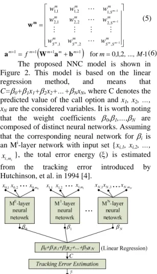
for 012 1 1 1 , ..., M-, , m fm m m m m+ ₌ + + ₊ + ₌ b a W a (6)

The proposed NNC model is shown in Figure 2. This model is based on the linear regression method, and means that

C=β0+β1x1+β2x2+…+βNxN, where C denotes the predicted value of the call option and x1, x2, …,

xN are the considered variables. It is worth noting that the weight coefficients β0,β1,…,βN are composed of distinct neural networks. Assuming that the corresponding neural network for βi is an Mi-layer network with input set {xi,1, xi,2, …,

i

m i

x_, }, the total error energy (ξ) is estimated

from the tracking error introduced by Hutchinson, et al. in 1994 [4]. 1 , 0 x 0 β 2 , 0 x 0 , 0 m x 1 β 1 , N x N β 3 , N x N m N x , 1 , 1 x x1,2 x1 m,1 C

Figure 2 Neural Network Coefficient Model

Tracking Error

The use of the tracking error as the performance measure is based on the no-arbitrage phenomenon. Let

V(t)=VS(t)+VB(t)+VC(t) be the value of the portfolio using our model, where VS(t), VB(t) and

VC(t) are the values of stocks, bonds and held call options at time t. The expected value of such a hedged option portfolio at the expiration date should be exactly zero. Let αti denote the

composition of the portfolio at time ti shown as

follows:

( )

( )

( )

( ) ( )

( )

( )

_{( ) ( ) ( ) ( )}

₍

₎

_⎥⎥ ⎥ ⎦ ⎤ ⎢ ⎢ ⎢ ⎣ ⎡ Δ − Δ − − Δ = ⎥ ⎥ ⎥ ⎦ ⎤ ⎢ ⎢ ⎢ ⎣ ⎡ = − − − − 1 1 1 i i i i B t t r i M i i i B i C i S t t t t S t V e t C t t S t V t V t V i i f i α (7) where

( )

( )

S t C t m i i _∂ ∂ = Δ . Cm(ti) is defined as the predicted call option value based on Model m, where m=BS or NNC. The initial case αt0 is

( )

( )

( )

( ) ( )

( )

( )

( )

(

)

⎥⎥ ⎥ ⎦ ⎤ ⎢ ⎢ ⎢ ⎣ ⎡ + − − Δ = ⎥ ⎥ ⎥ ⎦ ⎤ ⎢ ⎢ ⎢ ⎣ ⎡ = 0 0 0 0 0 0 0 0 0 t V t V t C t t S t V t V t V C S M B C S t α (8)

The total error energy ξm is defined as follows:

( )

(

V T

)

E e rT m f − = ξ (9)

Let ξ m (q) refer to the instantaneous error energy at iteration q by using model m. Used in a manner similar to the Least-Mean-Square (LMS) algorithm, the back-propagation algorithm applies a correction

w

njim , ,

Δ

to the synaptic weight

w

njim , , denoted by m i j

w

, in βn, n=0,1,2,…,N. ( ) ( ) ( ) ( )( ) ( )( ) w ( )( )q q q q C q C q V q V q w q m n i j n n NNC m n i j NNC , , , , ∂ ∂ ⋅ ∂ ∂ ⋅ ∂ ∂ ⋅ ∂ ∂ = ∂ ∂ β β ξ ξ (10) where ( ) ( ) ⎩⎨ ( )( ) ⎧ ≤ − > = ∂ ∂ − − 0 0 q V if e q V if e q V q T r T r NNC f f ξ (11) ( ) ( ) ( )( ) ( )( ) ( )( ) ( ) ( ) ( ) ( ) ( )C( )q t t S q C q V e q C q V q C q V q C q V q C q V i i B t t r C B S i i f ∂ Δ ∂ + ∂ ∂ = ∂ ∂ + ∂ ∂ + ∂ ∂ = ∂ ∂ − −−1 1 (12) ( ) ( ) ⎩⎨ ⎧ = = = ∂ ∂ N 1,2,..., n if x n if q q C n n 0 1 β (13) The adjustment to

w

njim , , is similar to the

traditional back-propagation algorithm, because each βn is defined by a complete neural network. So, ( ) ( ) ( ) ( ) ( ) ⎪⎩ ⎪ ⎨ ⎧ ≠ ⋅ ′ = ⋅ ′ = ∂ ∂

∑

n k j m n j k n j m n i j n M m if q a w M m if q a w q ϕ ϕ β , , , , (14)

Finally,

Δ

w

n_j,,_im is illustrated in Equation (15).

( ) m n i j NNC m n i j w q w _, , , , _∂ ∂ ⋅ − = Δ η ξ (15)

3. Results

of Experiment

To avoid losing reality, our experimental data are obtained from Taiwan Stock Index Commodity (TIMEX) index options instead of using artificial simulated data. These data are European-style options. It means that they are exercised only on the option expiration date, and the payoff is determined by the Taiwan Stock Index on the option maturity date. There are 841 samples chosen from the TIMEX during 2004, which are further divided into training and testing sets with corresponding ratios of 80% and 20%.

The simulation programs are written in Borland C++ Builder 6.0 run on a Microsoft Windows XP professional platform. The considered variables set (x1, x2, x3, x4, x5) used in our NNC model is (S, K, rf, T, σ), which is introduced by the BS model illustrated in Table

1. The corresponding input set for βi is shown in Table 2.

Table 2. The Corresponding Input Setfor βi βi Input Set β0 (K, T) β1 (K, T, S, V) β2 (K, T, S) β3 (K, T+1, T+2, T+3) β4 (K, T+1, T+2, T+3) β5 (K, T, 1 − i t σ , 2 − i t σ , 3 − i t σ )

The configuration of each neural network is presented in Table 3 of our NNC model. Table 3. The Configuration of Each Neural

Network

Parameter Value No. of Hidden Layers 2 No. of Neurons in each Hidden Layer 6 Activation Function (Hidden Layer) Sigmoid Activation Function (Output Layer) Linear Learning Rate 0.01 No. of Epochs 1000

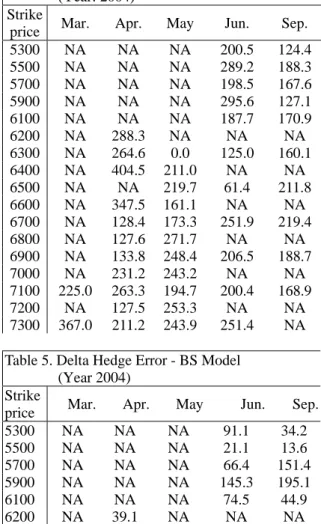
The derived absolute delta-hedging errors of the NNC and BS models are shown in Table 4 and Table 5, respectively. The total error energies are ξNNC=200.56 and ξBS==714. These

results show that our proposed NNC model performs better than the BS model.

Table 4. Delta Hedge Error – NNC model (Year: 2004)

Strike

price Mar. Apr. May Jun. Sep. 5300 NA NA NA 200.5 124.4 5500 NA NA NA 289.2 188.3 5700 NA NA NA 198.5 167.6 5900 NA NA NA 295.6 127.1 6100 NA NA NA 187.7 170.9 6200 NA 288.3 NA NA NA 6300 NA 264.6 0.0 125.0 160.1 6400 NA 404.5 211.0 NA NA 6500 NA NA 219.7 61.4 211.8 6600 NA 347.5 161.1 NA NA 6700 NA 128.4 173.3 251.9 219.4 6800 NA 127.6 271.7 NA NA 6900 NA 133.8 248.4 206.5 188.7 7000 NA 231.2 243.2 NA NA 7100 225.0 263.3 194.7 200.4 168.9 7200 NA 127.5 253.3 NA NA 7300 367.0 211.2 243.9 251.4 NA Table 5. Delta Hedge Error - BS Model

(Year 2004) Strike

price Mar. Apr. May Jun. Sep. 5300 NA NA NA 91.1 34.2 5500 NA NA NA 21.1 13.6 5700 NA NA NA 66.4 151.4 5900 NA NA NA 145.3 195.1 6100 NA NA NA 74.5 44.9 6200 NA 39.1 NA NA NA

6300 NA 73.7 0.0 51.2 150.4 6400 NA 62.4 218.9 NA NA 6500 NA NA 415.5 159.9 333.6 6600 NA 1912.6 2305.9 NA NA 6700 NA 2727.1 1830.4 2017.4 1890.3 6800 NA 2813.4 974.5 NA NA 6900 NA 1458.7 1382.0 1463.8 1648.3 7000 NA 206.0 513.6 NA NA 7100 28.5 101.7 356.3 260.8 262.9 7200 NA 54.3 139.2 NA NA 7300 0.7 127.2 126.9 176.1 NA

4. Conclusions

Generally speaking, financial data forecasting is always difficult because it is greatly influenced by economic, international and political events. The option pricing model tends to be more popular with financial institutions for both speculative and hedging purposes. The Black-Scholes model is a well-known option pricing model based on certain specific assumptions. However, past studies have shown that the Black-Scholes model cannot effectively capture the nonlinear behavior of option prices if real options data is applied. In this article, we therefore introduce a neural network coefficient (NNC) model to estimate option pricing to improve the tracking of error performance used to measure hedging capability. This model uses the variables included in the BS model and combines them with linear regression to evaluate the option value. To capture the nonlinear behavior of option prices with a high degree of accuracy, each coefficient in the linear regression model is produced by a neural network. The empirical results show that the derived average absolute delta-hedging errors of the NNC and BS models are ξNNC=200.56 and ξBS==714, respectively. It

is obvious that our proposed NNC model performs better hedging capability than the BS model.

References

[1] N. Burgess and A-P. N. Refenes, “Modelling non-linear moving average processes using neural networks with error feedback: An application to implied volatility forecasting,” Signal Processing, 74:89-99, 1999.

[2] A-P. N. Refenes and W. T. Holt, “Forecasting volatility with neural regression: A Contribution to model adequacy,” IEEE Transactions on Neural Networks, 12:850-864, 2001.

[3] P. Lajbcygier, “Improving option pricing with the product constrained hybrid neural network,” IEEE Transactions on Neural Networks, 15:465-476, 2004.

[4] J. M. Hutchinson, A. W. Lo and T. Poggio, “A nonparametric approach to pricing and hedging derivative securities via learning networks,” Journal of Finance, 49:851-889, 1994.

[5] H. Amilon, “A neural network versus Black-Scholes: A comparison of pricing and hedging performances,” Journal of forecasting, 22:317-335, 2003.

[6] J. Bennell and C. Sutcliffe, “Black-Scholes versus neural networks in pricing FTSE 100 options,” Working Paper 00-156, University of Southampton - Department of Accounting and Management Science, 2003.

[7] S. A. Hamid and Z. Iqbal, “Using neural networks for forecasting volatility of S&P 500 index futures prices,” Journal of Business Research, 57:1116-1125, 2004. [8] R. Gencay and M. Qi, “Pricing and hedging

derivative securities with neural networks: Bayesian regularization, early stopping, and bagging,” IEEE Transactions on Neural Networks, 12:726-734, 2001.

[9] M. J. Morelli, G. Montagna, O. Nicrosini, M. Treccani, M. Farina and P. Amota, “Pricing financial derivatives with neural networks,” 338:160-165, 2004.

[10] J. Yao, Y. Li and C. L. Tan, “Option price forecasting using neural networks,” International Journal of Management Science, 28:455-466, 2000.

[11] A. Carverhill and T. H. F. Cheuk, “Alternative neural network approaches for option pricing and hedging,” Working paper, Dec. 2003.

[12] D. Ormoneit, “A regularization approach to continuous learning with an application to financial derivatives pricing,” Neural Networks, 12:1405-1412, 1999.

[13] G. Bakshi, C. Cao, and Z. Chen, “Empirical performance of alternative option pricing models,” Journal of Finance, LII:2003-2049, 1997.

[14] F. Black and M. Scholes, “The pricing of options and corporate liabilities,” Journal of Political Economy, 81:637-659, 1973.

行政院國家科學委員會補助團隊參與國際學術組織會議報告

年 月 日

報告人姓名

柯博昌

服務機構

高雄應用科技大學

資管系

_職稱

副教授

中文：串接式類神經網路在財務時間序列模型與預測之研究

會議正式名稱

英文：The 4

th

International Conference on Computational Intelligence in

Economics and Finance（CIEF’2005）

會 議 時 間

自 94 年 7 月 21 日至 94

年 7 月 26 日

地點（國、州、城市）

美國猶他州鹽湖城

報告內容應包括下列各項：

一、 參加會議經過

CIEF2005 是計算智慧於經濟與財務之國際型學術研討會，本屆研討會自 94 年 7 月 21 日至 26 日於

美

國猶他州鹽湖城

舉行。每 1 年集合全球

資訊科技

的尖端學者參與盛會。並經過嚴格的專業審查，收錄目 前相關計算智慧於經濟與財務理論與應用的研究論文，具有崇高的學術地位。全世界的資訊科技與財務經 濟應用研究學者，皆以能在本研討會發表論文為榮。

二、 與會心得

會議分成 20 個 Sections， Invited Keynote Speaker 1 位(

美國 Brandeis 大學 Blake LeBaron 教授在代理

人基計算財務學（agent-based computational finance, ABCF）中，享有盛名。今年又正值代理人基計

算財務學發展的十週年，LeBaron 教授將以「How real are artificial stock markets」為題講演，對

ABCF 的十週年做一回顧與前瞻

)。Tutorial speakers 2 位(

分別由英國伯明罕大學的 Colin Frayn 博

士講授 Genetic Programming in Finace 以及西班牙巴塞隆納大學（Universitat Autònoma de Barcelona）

的 Michael Creel 博士講授 Setup and Use of a Non-Dedicated Cluster for Paralle Computing with

Examples

)。發表的研討會論文近 90 篇。來自台灣被接受的文章有近 30 篇 Conference paper，本人的文章即 是正式的 Conference paper。在全程的參與過程中，聆聽全球電腦尖端學者在計算智慧於經濟與財務應用的研

究成果，受益良多。本人於 7 月 25 日上午發表的「

Cascading Neural Network Approach to Financial Time

Series Modeling and Forecasting

」論文以及主持兩場會議時, 引起台下聽眾的熱烈興趣，本人亦與台下聽眾 熱烈討論以及會後的進一步資訊交流，經由參與本國際會議，一方面發表個人的研究成果，另一方與專家學 者討論中獲得更新的資訊交流, 對未來研究將有更大的助益。

三、 考察參觀活動（無是項活動者省略）

無

四、 建議事項

國內相同領域的學者應多支持此類似之國際會議，一方面發表國人的科技研究成果，同時與國際知名 學者交流, 吸取更豐富的知識與資訊, 以儲備不久將來可在國內舉辦此類國際會議的能量。

五、 其他