1036 Am J Epidemiol 2003;158:1036–1038 American Journal of Epidemiology
Copyright © 2003 by the Johns Hopkins Bloomberg School of Public Health All rights reserved
Vol. 158, No. 11 Printed in U.S.A. DOI: 10.1093/aje/kwg268
Lee Responds to “Making the Most of Genotype Asymmetries”
Wen-Chung Lee
From the Graduate Institute of Epidemiology, College of Public Health, National Taiwan University, Taipei, Taiwan, Republic of China.
Received for publication September 10, 2003; accepted for publication September 16, 2003.
I am grateful to Dr. Weinberg for her insightful commentary (1) on my paper (2). Weinberg is looking forward eagerly to a day when researchers will be able to search the whole genome for susceptibility loci for complex diseases (1). Likewise, I notice with excitement that the conventional “risk factor” epidemiology as we know it has undergone a profound change. Moving into this postgenomic era, epidemiology can mean gene-mapping business, no less truly than it has been for so long about odds ratios and confidence intervals for, for example, smoking and lung cancer.
To obtain a weighting scheme for the various family configurations encountered in actual practice, the Di is
defined as the allele count for the case (Ci) minus the
allele count for the following: 1) nontransmitted, Ni
(case-parents data); 2) imputed nontransmitted, (case-sibling data); 3) spouse, Si (case-spouse data); and 4)
im-puted spouse, (case-offspring data), where the “non-transmitted” refers to the parental alleles not transmitted to the case (1), the “imputed nontransmitted” has an al-lele count of , where the Bi is the mean
al-lele count of the control siblings, and the spouse and the imputed spouse are defined the same as in my paper (2). The Dis defined in this way all have the same “mean” (e1 in my paper (2)) under the alternative hypothesis, irre-spective of family configurations. The statistical effi-ciencies of the various family configurations are then in proportion to the inverses of their respective “variances” (e2 in my paper (2)).
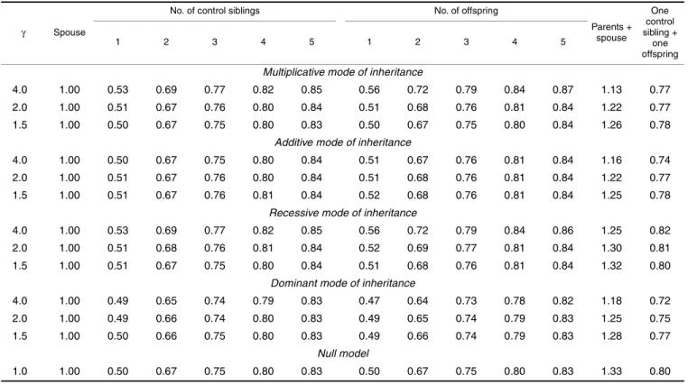
Table 1 presents the relative efficiencies for the various family configurations (relative to case-parents data). Note that, in this paper, the disequilibrium test (1), but not the transmission/disequilibrium test (2), was applied to the case-parents data. To be brief, I present only the case with the allele frequency set at P = 0.1. It is of interest to note the following. First, the case-spouse data and the case-parents data have exactly the same efficiency. Second, the offspring data and the
case-sibling data have roughly the same relative efficiency, when the number per family of offspring and the number per family of control siblings are equal. Third, the rela-tive efficiency of the case-offspring (case-sibling) data with one offspring (control sibling) per family is ~0.5. These findings largely confirm Weinberg’s speculations (1).
In addition, I agree with Weinberg (1) that the informa-tion from the following two lines of relatives can be inte-grated to improve the power of the disequilibrium test: line I, the parents or, if the parents are missing, the control siblings; and line II, the spouse or, if the spouse is missing, the offspring. The penultimate column of table 1 presents the relative efficiencies (also calculated from e2 in my paper (2)) for a Di, averaged from
case-parents and case-spouse data, and the last column, the relative efficiencies from one control sibling and one offspring. It is of interest to note that the relative effi-ciencies are less than 2.00 for parents plus spouse. (Having two controls does not make the case twice as informative). Moreover, the relative efficiencies are less than 1.00 for one control sibling plus one offspring. (Two haploids do not make a whole diploid control). The values are larger than the corresponding values for two control siblings or two offspring, though. (Having two lines of relatives is better than having only one).
The variance formula simplifies considerably under the null. We have, dropping the subscript i, Var(D) = Var(C – N) = Var(C) + Var(N) = 4P(1 – P), for case-parents data. Likewise, Var(D) = Var(C – S) = Var(C) + Var(S) = 4P(1 – P),for case-spouse data. Because the numbers of “identical by descent” (3) for a sibling pair are 2 (probability = 0.25), 1 (probability = 0.5), and 0 (probability = 0.25), we have Cov(B1, B2) = Cov(C, B1) = 0.25 × 2P(1 – P) + 0.5 × P(1 – P) + 0.25 × 0 = P(1 – P), with
B1 and B2 being the allele count for the first and the second control siblings, respectively. Thus, for case-sibling data with x control case-siblings per family,
Reprint requests to Dr. Wen-Chung Lee, Graduate Institute of Epidemiology, National Taiwan University, No. 1, Jen-Ai Road, 1st Section, Taipei 100, Taiwan, Republic of China (e-mail: wenchung@ha.mc.ntu.edu.tw).
Nˆi
Sˆi
Lee Responds to Weinberg 1037
Am J Epidemiol 2003;158:1036–1038 Similarly, we can show that
for case-offspring data with y offspring per family.
Treating case-parents data as case-sibling data with x = ∞ and case-spouse data as case-offspring data with y = ∞, the variance (under the null) of a weighted average of the two lines of relatives (superscripts, I and II) is
where Ok is the allele count for the kth offspring. With the use of the identical-by-descent probabilities again (for siblings,
parent-offspring, and uncle-nephew pairs) (3), the last term can be shown to be t(1 – t) × 4P(1 – P). Thus, the variance is a quadratic function of t and has a minimum value of
when
TABLE 1. Relative efficiencies for the various family configurations (relative to case-parents data)
γ Spouse
No. of control siblings No. of offspring
Parents + spouse One control sibling + one offspring 1 2 3 4 5 1 2 3 4 5
Multiplicative mode of inheritance
4.0 1.00 0.53 0.69 0.77 0.82 0.85 0.56 0.72 0.79 0.84 0.87 1.13 0.77
2.0 1.00 0.51 0.67 0.76 0.80 0.84 0.51 0.68 0.76 0.81 0.84 1.22 0.77
1.5 1.00 0.50 0.67 0.75 0.80 0.83 0.50 0.67 0.75 0.80 0.84 1.26 0.78
Additive mode of inheritance
4.0 1.00 0.50 0.67 0.75 0.80 0.84 0.51 0.67 0.76 0.81 0.84 1.16 0.74
2.0 1.00 0.51 0.67 0.76 0.80 0.84 0.51 0.68 0.76 0.81 0.84 1.22 0.77
1.5 1.00 0.51 0.67 0.76 0.81 0.84 0.52 0.68 0.76 0.81 0.84 1.25 0.78
Recessive mode of inheritance
4.0 1.00 0.53 0.69 0.77 0.82 0.85 0.56 0.72 0.79 0.84 0.86 1.25 0.82
2.0 1.00 0.51 0.68 0.76 0.81 0.84 0.52 0.69 0.77 0.81 0.84 1.30 0.81
1.5 1.00 0.51 0.67 0.75 0.80 0.84 0.51 0.68 0.76 0.81 0.84 1.32 0.80
Dominant mode of inheritance
4.0 1.00 0.49 0.65 0.74 0.79 0.83 0.47 0.64 0.73 0.78 0.82 1.18 0.72
2.0 1.00 0.49 0.66 0.74 0.80 0.83 0.49 0.65 0.74 0.79 0.83 1.25 0.75
1.5 1.00 0.50 0.66 0.75 0.80 0.83 0.49 0.66 0.74 0.79 0.83 1.28 0.77
Null model
1.0 1.00 0.50 0.67 0.75 0.80 0.83 0.50 0.67 0.75 0.80 0.83 1.33 0.80
Var D( ) Var C( –Nˆ) 4 Var C Bj j=1 x
∑
– ⁄x × = = 8P 1( –P) 4 x2 ----×[x×2P 1( –P) x x 1+ ( – ) Cov B× ( 1,B2)] 8 Cov C B– × ( , 1) + = x+1 x ---×4P 1( –P). = Var D( ) y+1 y ---×4P 1( –P) = Var tD[ I+(1–t)DII] [t2(x+1) x⁄ +(1–t)2(y+1) y⁄ ] 4P 1 P× ( – ) 8t 1( –t) Cov C Bj j=1 x∑
⁄x – C Ok k=1 y∑
⁄y – , , × + = 1–xy⁄[4 x( +1) y 1( + )] x⁄(x+1) y+ ⁄(y+1) xy– ⁄[(x+1) y 1( + )] ---×4P 1( –P),1038 Lee
Am J Epidemiol 2003;158:1036–1038 The last row of table 1 presents the relative efficiencies
calculated from these formulas. It can be seen that the approximation is satisfactory as long as the risk parameter, γ, is not too far away from its null value of 1.0. Therefore, the following weighted disequilibrium test is proposed (with the subscript, i, denoting the ith family):
with
and
which is distributed as a 1-degree-of-freedom chi-square distribution under the null.
REFERENCES
1. Weinberg CR. Invited commentary: making the most of geno-type asymmetries. Am J Epidemiol 2003;158:1033–5. 2. Lee WC. Genetic association studies of adult-onset diseases
using the case-spouse and case-offspring designs. Am J Epide-miol 2003;158:1023–32.
3. Sham P. Statistics in human genetics. New York, NY: Oxford University Press, Inc, 1998:209.
t x⁄(x+1)–xy⁄[2 x( +1) y 1( + )] x⁄(x+1) y+ ⁄(y+1) xy– ⁄[(x+1) y 1( + )] ---. = X2 wi I Di I wi II Di II + ( ) i=1 n