The FPGA Design of the Scan Conversion for Multimedia

全文

(1)Int. Computer Symposium, Dec. 15-17, 2004, Taipei, Taiwan.. The FPGA Design of the Scan Conversion for Multimedia GUO-CHIUAN WANG AND MING-CHIEH TSAI Department of Electrical Engineering Tatung University processior@yahoo.com.tw. Abstract-Image scaling is important in conversion between different formats such as VGA, NTSC and HDTV. As an application, we consider a scan formats, such as a VGA mode into 720p as a target signal format. In this paper proposes the design of a scan converter based on propose adaptive cubic convolution (ACC), which was modeled in verilog and implemented with an FPGA chip. The algorithm (ACC) exhibits of information loss when compared with the traditional interpolation algorithms, particularly in the edge regions. To realize the chip of this design, we use verilog, Xilinx tool and Synopsys library to design and simulate. We use FPGA(XC2V 1000 0.18μm CMOS process) to implement it. The gate count is 825,186. The operating clock rate is 25MHz, 50MHz and 75 MHz, with embedded memory requirement of 16kB. Keywords: adaptive cubic convolution (ACC) 1. Introduction A high-performance scaling algorithm that can scale an image without introducing much distortion will allow us to transmit image data using a small image size format while maintaining perceptual quality. For example, if a VGA format picture is to be displayed on HDTV monitors. Image scaling is also sometimes referred to as spatial up-conversion. Scaling techniques that are commonly used include simple pixel replication, bilinear interpolation and cubic convolution interpolation. These techniques can be considered as separable FIR filters [1] of two, three and seven taps, respectively, in each dimension. Video scaling finds use in conversion from one format to another such as NTSC to PAL, PAL to SECAM, HDTV, especially with emerging flat panel displays. For instance, if VGA format (640x480 pixels) is to be converted into 720p format (1280x720 pixels), it needs up scaling by a ratio of 2:1.5. The hardware implementations based on FPGA and ASIC can exploit pipelined and massively parallel processing, resulting in faster and cost effective solutions. ASIC designs are suitable if high volume production is envisaged. However, in the research and development phase, for rapid prototyping of a new design and for dynamic reconfigurability, FPGA is the right choice. Further, FPGA implementation is cost effective for low volume applications. The following sections present the algorithm, architecture and its FPGA implementation of the proposed method for. video scaling. 2. Interpolation of an edge We show in this section that the ACC technique is able to reduce the error when interpolating edge points. To this purpose, we need a model for the edge; those typically used in the literature are the step, the linear ramp, and the sigmoid [2]. Step edges are extremely rare in real images, since any lowpass effect in the acquisition process causes them to change into sigmoidal functions. In the following, we use a sigmoid as a model for the edge. Let the true data be represented by the sigmoidal function. f ( x ) = 255 (1 + e − cx ) . (1) The edge location is x = 0 ; its steepness is controlled by the constant c and its amplitude is 255. We had shown the sigmoidal function in Figure 1. We may obtain an estimate for the function at position using the cubic convolution Interpolation in [3]: Figure 2 shows the behavior of this error as an unction of x and s and for different values of c the values of c are selected in order to see the effects on edges of different width, we set c = 3 and c = 4 . In Figure 2,if the curve is sharpest then error is large than curve is smothering. 3. Description of our algorithm The capability to digitally interpolate images to different resolution with good image quality is important in many applications. Using the adaptive cubic convolution (ACC) to the local property of the sampled data is critical factor in improving the perceived quality of the scaled image. In this paper, we. 1273. Figure 1 sigmoidal function.

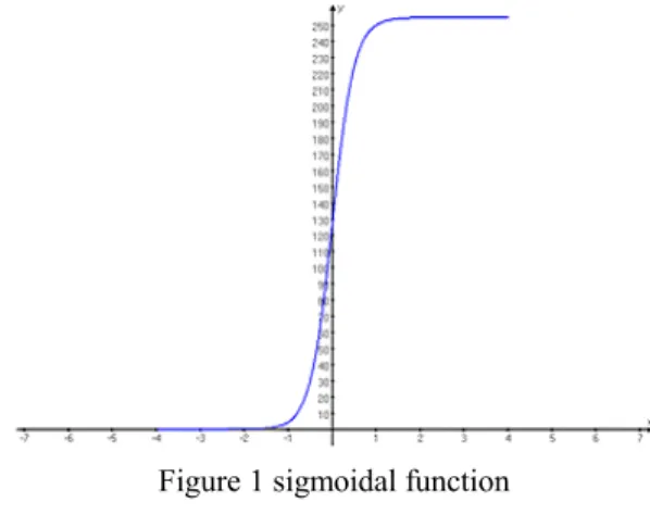
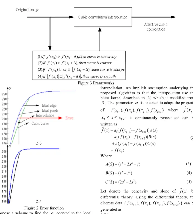
(2) Int. Computer Symposium, Dec. 15-17, 2004, Taipei, Taiwan.. Original image Cubic convolution interpolation Adaptive cubic convolution. (1) If f ′( x0 ) > f ′( x0 + ∆ ), then curve is concavity (2) If f ′( x0 ) < f ′( x0 + ∆ ), then curve is convex (3) If f ′( x0 ). or. f ′( x0 + ∆) , then curve is sharpe. (4) If f ′( x0 ) ≅ f ′( x0 + ∆) , then curve is smooth. Figure 3 Frameworks interpolation. An implicit assumption underlying the proposed algorithm is that the interpolation use the basis kernel described in [3] which is modified from [3]. The parameter a is selected to adapt the property of. f ( xk −1 ), f ( xk ), f ( xk +1 ), f ( xk + 2 ). where. ) f ( xk ). xk ≤ x ≤ xk +1 is continuously reproduced can be written as ) f ( x ) = a1 ( f ( xk −1 ) − f ( xk +1 )) A( s ). + a2 ( f ( xk ) − f ( xk + 2 )) B ( s ). (2). + a ( f ( xk ) − f ( xk +1 ))C ( s ) + f ( xk ) Where. Figure 2 Error function propose a scheme to find the a adapted to the local property of the sampled data in such a way that the concavity and slope of the produced pixels using the selected a is coincided with that of the neighbor pixels. Since real data is not stationary, the adaptation of the parameter is performed in each sub-pixel of the data to be processed. With these considerations in mind, we have developed a new cubic convolution method for image interpolation. Figure 3 shows the framework within which the parameter a is adapted for four pixels { f ( xk −1 ), f ( xk ), f ( xk +1 ), f ( xk + 2 ) }, where f ( xk ) ' s. A( S ) = ( s 3 − 2 s 2 + s ). (3). B( S ) = ( s3 − s 2 ). (4). C ( S ) = (2s 3 − 3s 2 ). (5). ) Let denote the concavity and slope of f ( x) by differential theory. Using the differential theory, the discrete data { f ( xk −1 ), f ( xk ), f ( xk +1 ), f ( xk + 2 ) } can be generated as follows.. f ′( xk ) ≅ ( f ′( xk +1 ) − f ′( xk −1 )) / ∆ f ′( xk +1 ) ≅ ( f ′( xk + 2 ) − f ′( xk )) / ∆ Let ∆ = 1 , then: f ′( xk ) ≅ ( f ′( xk +1 ) − f ′( xk −1 )) f ′( xk +1 ) ≅ ( f ′( xk + 2 ) − f ′( xk )). represent the original data. The proposed system consists of an adaptation of a and cubic convolution. 1274. (6). (7). ⎧convex if f ′( x0 ) < f ′( x0 + ∆) ⎨ ⎩concavity if f ′( x0 ) > f ′( x0 + ∆). ⎧error ⇒ large ⎨ ⎩error ⇒ small. if f ′( x0 ) or f ′( x0 + ∆) So if f ′( x0 ) ≅ f ′( x0 + ∆ ).

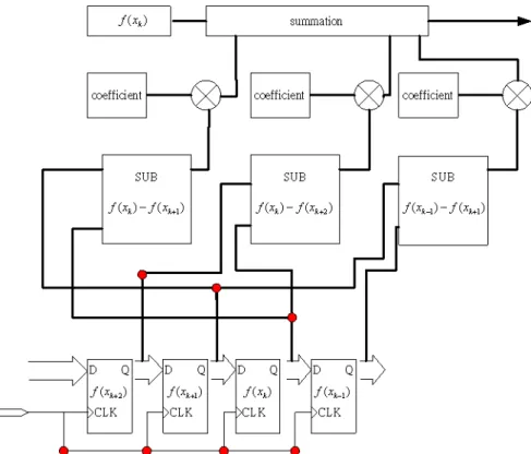
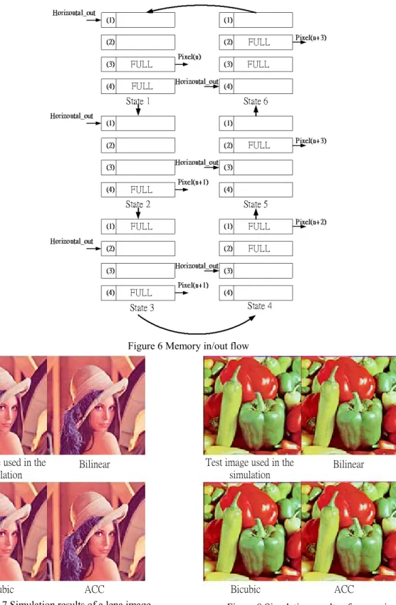
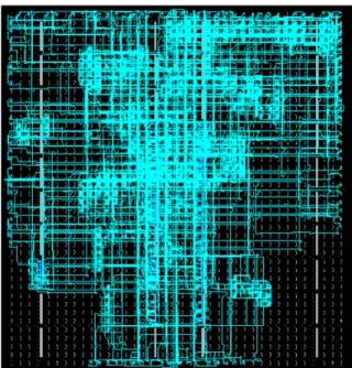
(3) Int. Computer Symposium, Dec. 15-17, 2004, Taipei, Taiwan.. we understand A(s), B(s) and C(s) is constant function; a1 and a2 are parameters. In general equally a1 = a2 = −. 1 , but I can use difference theory which 2. decide cubic kernel function. We proposed adaptive tune cubic kernel function algorithm is performed as in Table 1. Table 1 Adaptive a1 and a2. 4.Hardware architecture A novel architecture suitable for FPGA implementation of a scalar is presented in this section. The demand for the ability to display video signals on the high-resolution monitor has been increasing. Scan conversion process (scalar) is required for resizing the source video data to fit the target format. In this paper, we use FPGA implementation for adaptive cubic interpolation that is better performance than the other traditional interpolation manners. 4.1Scan Conversion structure and architecture The scalar using the adaptive cubic interpolation consist of 5 blocks: Memory block, horizontal scalar, vertical scalar, control signal and clock Synthesizer, as in Figure 4 The detailed explanation of each block is given below. 4.2. Scalar blocks In this paper we propose a new algorithm (adaptive cubic interpolation) is performed in the scalar block. We use verilog language and DSP FIR-FILTER translation cubic kernel function. cubic kernel function is a mathematical representation of a fundamental polynomial. Polynomial can be implemented several ways in the FPGA. We can use a 4-tap, 8-Bit Finite impulse Response (FIR) filter to achieve Equation [3], as shown in Figure 5. 4-tap FIR filter has the data flow processing as follows. The input data is registered in D Flip-Flops and then serially shifted LSB first at the clock rate. The output D Flip-Flops to subtraction produces three equations f ( xk −1 ) − f ( xk +1 ) , f ( xk ) − f ( xk + 2 ) and f ( xk ) − f ( xk +1 ) . Finally, the three-equation multiply coefficient (A (S), B (S), C (S)), and then plus the f ( xk ) . 4.3. Memory block. When input data are inserted to the horizontal block, memory is required to store for the interpolation and we total use 16kbyte.There,we use Virtex-II Family provides block memory. The dedicated RAM provides very high speed, comparable to discrete memories or ASIC memory cores. 4.4. Control signal The block is control memory read/write, select memory line and memory address. We use counter and compare to achieved select memory and address signal. The select input and output of memory block conditions are shown in Figure 6.In Figure 6, pixels form horizontal scalar block input to memory1 and memory3 to vertical block. The principle of state1~state6 above will be the reason by analogy. 4.5. Digital Frequency Synthesizer block The block is used to solve a timing problem and a wide rage of output frequencies when we execute the scan converter. Delay cells constitute this block to control the phase of a clock provided to each block. The block generates three frequencies 25MHz, 50MHz and 75MHz to horizontal and vertical blocks. 5. Computer simulation results The low-resolution image is obtained by down sampling the image by 2 in horizontal and vertical directions to yield a 256 × 256 low-resolution image. This image is then interpolated to its original resolution of 512 × 512 . The peak signal-to-noise (PSNR) between the original image and the interpolated images is then estimated. We proposed adaptive image interpolation method is tested on the same image for bilinear, bicubic and cubic spline methods. The PSNR results are tabulated in Table 2 Results show that the proposed adaptive weighted image interpolation yields better results that the traditional interpolation techniques. 6. Implement results We have designed the proposed adaptive cubic interpolation by using a verilog tool we verified it through timing simulation. Figure 11 shows the placement and route circuit results of the proposed circuits using an FPGA(XC2V 1000 0.18μm CMOS process, 3.3V power supply) to implement it. The implement result show that the adaptive cubic interpolation (ACC) image scalar has occupied with 825,186 gate count. 7. Conclusion In this paper, we proposed an adaptive cubic interpolation and implementation it. The present design is capable of working at 75MHz and has about 826,626 gate counts, with embedded memory requirement of 16kB.However, the adaptive cubic convolution algorithm can overcome those disadvantages (blocking, blurring) because the proposed method adaptive performs interpolation through the correlation of. 1275.

(4) Int. Computer Symposium, Dec. 15-17, 2004, Taipei, Taiwan.. performs interpolation through the correlation of neighbored pixels. References [1]Y.Wang and S. K. Mitra,”Image representation using block pattern models and its image processing applications,”IEEE Trans.Pattern Anal.Machine Intell.,vol.15,pp.321-336, Dec. 1993. [2] Giovanni Ramponi(1998),” Warped Distance for Space-Variant Linear Image Interpolation,” IEEE transactions on image processing, vol. 8, pp.629-639 Dec.1978. [3]Robert G. Keys, “Cubic Convolution Interpolation for Digital Image Processing,” IEEE transactions on acoustics, speech, and signal processing, vol.29, pp.1153-1160, Dec.1981. [4] H. S. Hou and H. C. Andrews (1978), “Cubic splines for image interpolation and digital filtering,” IEEE Trans. Acoust., Speech, Signal Processing, vol. ASSP-26, pp. 508–517 Dec.1978.. [5] Shih-Chang Hsia ,Bin-Da Liu ,Jar-Ferr Yang ,and Chien-Hsin Huang(1996), “A Parallel video converter for displaying 4:3 image on 16:9 HDTV receivers,” IEEE transactions on circuits and systems for video technology, vol. 6 , pp. 695–699 Dec.1996. [6] Mohiy M.Hadhoud, Moawad I.Dessouk , and Fathi. E.Abd EI-Samie, “Adaptive Image Interpolation Based on Local Activity Levels ,” twentieth national radio science conference, vol.18-20, pp. 1 –8,Mar.2003. [7] Jung Woo Hwang and Hwang Soo Lee(2004), “Adaptive Image Interpolation Based on Local Gradient Features,” IEEE signal processing letters, vol.11,pp 359-362Mar. 2004. Figure 4 The scalar of architecture. Figure 5 Data flow diagram for 4-tap FIR Filter. 1276.

(5) Int. Computer Symposium, Dec. 15-17, 2004, Taipei, Taiwan.. Figure 6 Memory in/out flow. Test image used in the simulation. Bilinear. Bicubic. ACC. Test image used in the simulation. Bicubic. Figure 7 Simulation results of a lena image. Bilinear. ACC. Figure 8 Simulation results of pepper image. 1277.

(6) Int. Computer Symposium, Dec. 15-17, 2004, Taipei, Taiwan.. Test image used in the simulation. Bicubic. Bilinear. ACC. Figure 9 Simulation results of letter image. Figure 11 Placement and route circuit Test image used in the simulation. Bicubic. Bilinear. ACC. Figure 10 Simulation results of mutipage image Table 2 Simulation result of PSNR. 1278.

(7)