Hyperspectral Image Classification Using Dynamic Classifier Selection with Multiple Feature Extractions

全文

(1)Int. Computer Symposium, Dec. 15-17, 2004, Taipei, Taiwan.. Hyperspectral Image Classification Using Dynamic Classifier Selection with Multiple Feature Extractions Chia-Hao Pai(1), Bor-Chen Kuo(1), Tian-Wei Sheu(1), Jinn-Min Yang(2), and Li-Wei Ko(1) (1) Graduate School of Educational Measurement and Statistics, National Taichung Teachers College, Taichung, Taiwan (2) Department of Mathematics Education, National Taichung Teachers College, Taichung, Taiwan 906118@ms3.ntctc.edu.tw, kbc@mail.ntctc.edu.tw, ygm@ms3.ntctc.edu.tw, koliwei@pchome.com.tw classifiers with different feature extractions. Although there are many different combination strategies [4][5][9][13][14], only dynamic classifier selection based on local accuracy [14] is studied.. Abstract-Dynamic classifier selection is a strategy in multiple classifier system design. Feature extraction is one of the important procedures for mitigate Hughes phenomenon in hyperspectral image classification. Most papers have discussed the potential discriminatory information between different classifiers. In this paper, we try to exploit the discriminatory information extracted by different feature extractions for improving classification accuracy. Information is then combined by using a dynamic classifier selection strategy based on local information to make a consistency decision. This paper provides another thinking of constructing a multiple classifier system without additional classifier design by using multiple feature extraction.. 2. Multiple Classifier System Design The Multiple Classifier System (MCS) design cycle can be formulated as shown in Figure 1. In most papers, the ensemble overproduction focuses on the overproduction of classifiers. Since different feature extractions encapsulate complementary discriminatory information between each other. In this paper, the overproduction of both feature extraction and classifiers is considered and the step 2 and 3 are replaced by the dynamic classifier selection. We propose the following algorithm: Ensemble Overproduction Phase I: Use different feature extraction methods to generate informative feature ensembles. Ensemble Overproduction Phase II: Apply the ensembles obtained in Phase I to different classifiers and generate classifier ensembles. Dynamic Classifier Selection: For each point in the testing set, K nearest neighbors in the training set are used to calculate the local accuracies of classifiers. Then the classifier with the highest local accuracy is applied to classify the testing data. Local accuracy using K nearest neighbors is defined as: K ∑ yik local _ acc( j ) = C k =1 K ∑i=1 ∑k =1 yik. Keywords: Feature extraction, Dynamic classifier selection, Multiple classifier system.. 1. Introduction Many researches [4][5][8][9][13][14] show that combined classifier systems can outperform single classifier system. There are three basic combinations strategies: sequential combination [6], parallel combination [8], and dynamic classifier selection [5]. This study focuses on the third approach in hyperspectral data classification problem. Typically, design of a multiple classifier system considers the potential classification information between different classifiers. However, in hyperspectral data classification, feature extraction is an important factor that influences classification accuracy greatly. In this paper, the effects of three feature extractions, principal component analysis [1], Fisher’s linear discriminant analysis [3] and nonparametric weighted feature extraction [12], are explored. It is hard to decide which method is better than others. Therefore, how can we ensure that our classification system will produce optimal or suboptimal result? In this paper, we construct a multiple classifier system for combining different. K is the number of nearest neighbors surrounding the testing point j. In this study, K is set as 3. C is the number of classifiers. i=1,…,C. yik=1 if classifier i successfully classifies the neighbor k, otherwise, yik=0. Performance Evaluation: Evaluate algorithm performance by holdout accuracy.. 754.

(2) Int. Computer Symposium, Dec. 15-17, 2004, Taipei, Taiwan.. covariance matrix. A between-class scatter matrix is expressed as:. 1. Ensemble Overproduction. L. S bDA = ∑ Pi ( M i − M 0 )( M i − M 0 ) T i =1. 2 .Ensemble Choice. L. where M = E{ X } = P M ∑ i i 0 i =1. The optimal criterion of LDA algorithm is to find the first m eigenvectors corresponding to the largest m eigenvalues of ( S wDA ) −1 S bDA .. 3. Combiner Design. 4. Performance Evaluation. 3. Nonparametric Weighted Feature Extraction One of limitations of LDA is that it works well when data is normally distributed. A different between-class scatter matrix and a within-class scatter matrix were proposed in nonparametric weighted feature extraction (Kuo and Landgrebe, 2001; Kuo and Landgrebe, 2004) for improving this limitation. The optimal criterion of NWFE is also by optimizing the Fisher criteria, the between-class scatter matrix and the within-class scatter matrix are expressed respectively by L L n λ(ki , j ) (i ) NW (i ) (i ) (i ). Figure 1. MCS design cycle based on the overproduce and choose paradigm. [13]. 3. Feature Extractions and Classifiers A. Feature Extractions 1. Principal Component Analysis Principal component analysis (PCA) is defined by the transformation: Y =WT X where X ⊆ R n . W is an m-dimensional transformation matrix whose columns are the eigenvectors related to the eigenvalues computed according to the formula: λe = Se S is the scatter matrix (i.e., the covariance matrix): 1 1 N ( X − M )( X − M ) T , M = ∑ x i S= N −1 N i =1 where xi ∈ X , i=1,…,N, M is the mean vector of. S. L. ni. λ(ki ,i ). i =1. k =1. ni. ni. ( x k − M j ( x k ))( x k − M j ( x k )) T. ( x k(i ) − M i ( x k(i ) ))( x k(i ) − M i ( x k(i ) )) T. function of xk(i ) and local mean M j ( xk(i ) ) , and defined as: dist(xk(i) ,M j ( xk( i ) ) )−1 λ(i,j) = k n ∑ dist(xl(i),M j ( xl(i ) ) )−1 i. l =1. where dist (a, b) means the distance from a to b . If the distance between xk(i ) and M j ( x k(i ) ) is small then its weight λ(ki , j ) will be close to 1; otherwise,. λ(ki , j ) will be close to 0 and sum of total λ(ki , j ) for class i is 1. M j ( x k(i ) ) is the local mean of xk(i ) in the class j and defined as: dist(xk(i),xl( j ) )−1. nj. M j ( xk(i ) ) = ∑ wkl(i , j ) xl( j ) , where wkl(i,j) = l =1. ni. ∑ dist(x l =1. ,xl( j ) )−1. (i) k. The weight wkl( i , j ) for computing local means is a function of xk(i ) and xl( j ) . If the distance between. xk(i ) and xl( j ) is small then its weight wkl( i , j ) will be close to 1; otherwise, wkl( i , j ) will be close to 0 and sum of total wkl( i , j ) for M j ( x k(i ) ) is 1.. L. = ∑ Pi E{( X − M i )( X − M i ) | ω i } = ∑ Pi ∑ i T. i =1. j =1 k =1 j ≠i. In the formula, x k(i ) refers to the k -th sample from class i. The scatter matrix weight λ(ki , j ) is a. 2. Linear Discriminant Analysis The purpose of LDA is to find a transformation matrix A such that the class separability of transformed data ( Y ) is maximized. A linear transformation A from an n -dimensional X to an m -dimensional Y ( m < n ) is expressed by Y = AT X In LDA of statistics, within-class, between-class, and mixture scatter matrices are used to formulate criteria of class separability. LDA uses the mean vector and covariance matrix of each class. A within-class scatter matrix for L classes is expressed by (Fukunaga, 1990): L. i =1. S wNW = ∑ Pi ∑. X, N is the number of samples. This transformation W is called Karuhnen-Loeve transform. It defines the m-dimensional space in which the covariance among the components is zero. In this way, it is possible to consider a small number of “principal” components exhibiting the highest variance (the most expressive features).. DA w. = ∑ Pi ∑ ∑ i. Sb. In the NWFE criterion, we regularize S wNW to reduce the effect of the cross products of betweenclass distances and prevent singularity by. i =1. where Pi means the prior probability of class i , M i is the class mean and Σ i is the class i. 755.

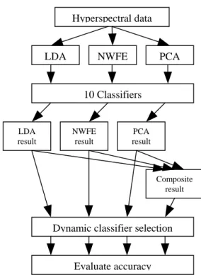
(3) Int. Computer Symposium, Dec. 15-17, 2004, Taipei, Taiwan. 0.5S wNW + 0.5diag ( S wNW ). Hyperspectral data. Hence, the features extracted by NWFE are the first m eigenvectors corresponding to the largest m eigenvalues of ( S wNW ) −1 S bNW .. LDA. B. Classifiers Ten classifiers described in Table 1. are used to construct the multiple classifier system. All classifiers are implemented in a Matlab toolbox for pattern recognition, called PR-tools. [2].. NWFE. PCA. 10 Classifiers. LDA result. Table 1. Classifiers used in this study. Notation Classifiers Normal densities based quadratic qdc classifier Train feed forward neural network bpxnc classifier by backpropagation parzenc Parzen density based classifier svc Support vector classifier Pseudo-Fisher support vector pfsvc classifier loglc Logistic linear classifier knnc1 k-nearest neighbor classifier.(k=1) knnc20 k-nearest neighbor classifier.(k=20) neurc Automatic neural network classifier Construct binary decision tree treec classifier. NWFE result. PCA result. Composite result. Dynamic classifier selection. Evaluate accuracy Figure 2. Experiment design in this study.. 5. Results and Findings To simply result graphs, only the performances of the top 5 single classifiers using 2 to 6 features are shown in Figure 3, 4, and 5. Figure 6 shows the classification accuracy obtained by using dynamic classifier selection strategy. Table 2 shows single classifier accuracy using different feature space, multiple classifier accuracy using different feature space, and multiple classifier accuracy using composite feature space. The best single classifier is an arbitrary choice by authors because each single classifier has different performance at different number of features. The experimental result shows that the NWFE feature space produces better classification accuracy than LDA and PCA ones. The highest accuracy (0.939) occurs in the combination of NWFE and pfsvc. (number of features = 5). 4. Data Set and Experiment Design A. Training and Testing Data Training and testing data sets are selected from a small segment of a 191 bands hyperspectral image data. It was collected over the DC Mall maps which have seven classes (Roof, Street, Path, Grass, Trees, Water and Shadow) are selected to form training and testing data sets. There are 100 training samples and testing samples in each class. B. Experiment Design The experiment design is showed in Figure 1.. 756.

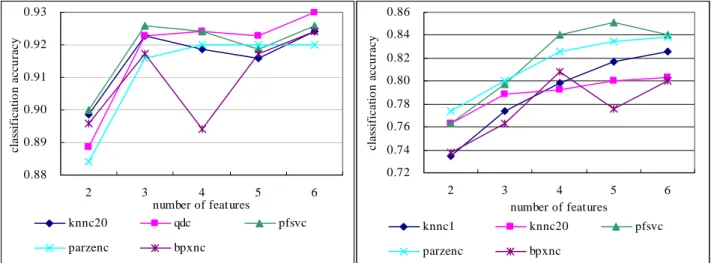
(4) Int. Computer Symposium, Dec. 15-17, 2004, Taipei, Taiwan.. 0.86. classification accuracy. classification accuracy. 0.93 0.92 0.91 0.90 0.89. 0.82 0.80 0.78 0.76 0.74 0.72. 0.88 2. 3. knnc20. 4 5 number of features qdc. parzenc. 2. 6 pfsvc. bpxnc. Figure 3. The performances of top 5 classifiers among 10 classifiers with LDA feature extraction.. 3. 4 5 number of features. knnc1. knnc20. parzenc. bpxnc. 6 pfsvc. Figure 5. The performances of top 5 classifiers among 10 classifiers with PCA feature extraction. 0.95. classification accuracy. 0.94. classification accuracy. 0.84. 0.93 0.92 0.91 0.90 0.89. 0.94 0.93 0.92 0.91 0.90. 2. 3. 4 5 number of features. knnc20. qdc. parzenc. bpxnc. 6. 2 LDA LDA+NWFE LDA+PCA. pfsvc. 3. 4 5 6 number of features NWFE NWFE+PCA LDA+NWFE+PCA. Figure 6. Dynamic classifier selection using local accuracy and 4 different feature extractions.. Table 2. Classification accuracy from dimension 1 to 6 in this study.. 6. Conclusions. Dynamic classifier selection. Best single classifier. Figure 4. The performances of top 5 classifiers among 10 classifiers with NWFE feature extraction.. Number of Features LDA (qdc) NWFE (parzenc) PCA (pfsvc) LDA NWFE PCA LDA+ NWFE NWFE+ PCA LDA+ PCA LDA+ NWFE +PCA. 1. 2. 3. 4. 5. 6. 0.616. 0.889. 0.923. 0.924. 0.923. 0.930. 0.821. 0.907. 0.937. 0.933. 0.939. 0.929. 0.596. 0.763. 0.797. 0.840. 0.851. 0.840. 0.613 0.834 0.701. 0.900 0.917 0.817. 0.929 0.939 0.820. 0.927 0.939 0.856. 0.926 0.939 0.859. 0.926 0.936 0.854. 0.840. 0.927. 0.939. 0.936. 0.930. 0.931. 0.837. 0.911. 0.934. 0.934. 0.937. 0.931. 0.819. 0.933. 0.936. 0.931. 0.930. 0.929. 0.869. 0.933. 0.940. 0.944. 0.937. 0.931. 757. According to the experimental results, the conclusions can be drawn: 1. Dynamic classifier selection strategy does not guarantee of producing better accuracy than a single classifier. But it is worth noting that the dynamic classifier selection strategy ensures to produce optimal or suboptimal classification accuracy. If we are not sure about which classifier is the best, dynamic classifier selection can be used for “stabilizing” classification accuracy. 2. Experimental results show that combining feature extraction methods slightly improve classification accuracy when the number of used features is smaller than 5 (see Figure 6). When the number of features is larger than 5, the classification accuracy of proposed algorithm in this study is not as good as single classifier with single feature extraction or dynamic classifier selection with single feature extraction. In our opinion, there exists.

(5) Int. Computer Symposium, Dec. 15-17, 2004, Taipei, Taiwan. Classification, ” IEEE Trans. on Pattern Analysis and Machine Intelligence, 24(7):893–904, 1998. [7] G.F. Hughes, ”On the mean accuracy of statistical pattern recognition,” IEEE Trans. Information Theory, 14(1), 55-63, 1968. [8] J. Kittler, M. Hatef, R.P.W. Duin and J. Matas, ”On Combining Classifiers,” IEEE Trans. on Pattern Analysis and Machine Intelligence, 20(3), 226–239, 1998. [9] L.I. Kuncheva, J.C. Bezdek and R.P.W. Duin, ”Decision templates for multiple classifier fusion: an experimental comparison.” Pattern Recognition, 34(2), 299–314, 2001. [10] B-C. Kuo and D.A. Landgrebe, ”Improved statistics estimation and feature extraction for hyperspectral data classification,” Technical Report, Purdue University, West Lafayette, IN., TR-ECE 01-6, December, 2001. [11] B-C. Kuo, D.A. Landgrebe, L-W. Ko, and C-H. Pai, ”Regularized Feature Extractions for Hyperspectral Data Classification,” International Geoscience and Remote Sensing Symposium, Toulouse, France, 2003. [12] B-C. Kuo, and D.A. Landgrebe, ”Nonparametric Weighted Feature Extraction for Classification,” IEEE Trans. on Geoscience and Remote Sensing, 42(5), 1096-1105, 2004.. [13] F. Roli, G. Giacinto, ”Design of Multiple Classifier Systems,” H. Bunke and A. Kandel (Eds.) Hybrid Methods in Pattern Recognition, World Scientific Publishing, 2002. [14] K. Woods, W.P. Kegelmeyer, K. Bowyer, ”Combination of Multiple Classifiers Using Local Accuracy Estimates, ” IEEE Transaction on Pattern Analysis and Machine Intelligence, 19(4), 405410, 1997.. potential discriminatory information between different feature extractions, but if the number of features is larger, the increasing noise may influence this information.. 7. Acknowledgements Authors would like to thank National Science Council for partially supporting this work under grant NSC-91-2520-S-142-001 and NSC-92-2521-S142-003.. References [1]. P.N. Belhumeur, J.P. Hespanha and D.J. Kriegman, ” Eigenfaces vs. Fisherfaces: Recognition Using Class Specific Linear Projection, ” IEEE Transaction on Pattern Analysis and Machine Intelligence, 19(7), 711-720, 1997. [2] R.P.W. Duin, PRTools, a Matlab Toolbox for Pattern Recognition, (Available for download from http://www.ph.tn.tudelft.nl/prtools/), 2002. [3] K. Fukunaga, Introduction to Statistical Pattern Recognition. San Diego: Academic Press Inc., ch9-10, 1990. [4] G. Giacinto and F. Roli, ”An approach to automatic design of multiple classifier systems. ” Pattern Recognition Letters, 22, 25–33, 2001. [5] G. Giacinto and F. Roli, ”Dynamic classifier selection based on multiple classifier behaviour.” Pattern Recognition, 34(9), 179–181, 2001. [6] N. Giusti, F. Masulli, and A. Sperduti, ”Theoretical and Experimental Analysis of a Two-Stage System for. 758.

(6)