Hardware Implementation of High-Throughput 3-D Rotation for Graphic Engine Using Double Rotation CORDIC Algorithm

全文

(1)Hardware Implementation of High-Throughput 3-D Rotation for Graphic Engine Using Double Rotation CORDIC Algorithm 宋志雲陳志炘 Tze-Yun Sung Chih-Sin Chen Department of Microelectronics Engineering Institute of Engineering Science Chung Hua University Hsinchu, Taiwan 300-12 bobsung@chu.edu.tw implementation and is applied to many signal processing tasks, such as sine and cosine generation, vector rotation, coordinate transformation and linear system solver. This algorithm is especially suitable for implementation of 3-D rotation. The CORDIC requires only shifters and adders, its realization on reconfigurable hardware platforms, especially on FPGA [5]. Thus, the 3-D rotation algorithm required in 3-D graphics can be realized with vector rotation, the CORDIC could be mainly used in this function block [6]. In this paper, the architecture of 3-D rotation with CORDIC algorithm is proposed, the proposed architecture is very suitable for VLSI implementation, and the computation complexity is also evaluated. The introduction of the new concept, double rotation CORDIC algorithm, improves throughput in the 3-D rotation, by up to 30% without any noticeable error occurrence. The view of observer in 2-D display system is performed by the 3-D central perspective method [7], the architecture of that is performed by 2-D CORDIC processors. The remainder of the paper is organized as follows. Section 2 reviews the 2-D CORDIC algorithm; section 3 presents the algorithm of CORDIC rotation in 3-D space, section 4 presents the double rotation CORDIC algorithm, the 3-D rotation with double CORDIC rotation algorithm is proposed in section 5, the 3-D central perspective method performed by CORDIC algorithm is proposed in section 6, VLSI architectures of 3-D rotation and perspective are described in section 7, The impact of new algorithms and architectures is presented and analyzed in section 8, and. Abstract High performance architectures can be design for data intensive and latency tolerant applications by maximizing the parallelism and pipelining at the algorithm. The hardware primitives for 3-D rotation for high throughput 3-D graphics and animation are presented in this paper. The primitives are based on the 2-D CORDIC algorithm, in contrast to conventional hardware for graphic engine. The accelerated architecture of the 3-D rotation based on double rotation CORDIC algorithm is also presented in this paper. The throughput is improved by more than 30%, but the additional hardware is required by less than 40%. The 3-D central perspective method for graphic engine is performed by double rotation CORDIC processors. The throughput is also improved by more than 30%. Keywords: 3-D rotation, double rotation CORDIC algorithm, graphic engine, 3-D perspective method, high-throughput. 1. Introduction Three dimensional rotation (3-D) is utilized in 3-D graphics, animation, and virtual reality applications [1] [2]. The rotations are applied to large number of points, which need quiet time consuming, but can be effectively parallel and pipelined. Moreover, 3-D computer hardware has been receiving great attention recently. The conventional hardware for 3-D rotation consists mainly of multipliers and accumulators. The CORDIC algorithm [3] [4] is widely recognized as well-suited for hardware 1.

(2) finally, the conclusion is given in section 9.. coordinates ( X i , Yi , Z i ) and spherical coordinates ( Ri ,θ i ,φi ) . The vector R can be rotated to become a new vector S which has cartesian coordinates ( X i +1 , Yi +1 , Z i +1 ) and spherical coordinates ( Ri ,θ i + α i ,φi + β i ) [8]. The relationship between the Cartesian coordinates and spherical coordinates of R and S are derived as follows: X i = Ri cosθ i sin φi (6) Yi = Ri sin θ i sin φi (7) Z i = Ri cos φi (8) X i +1 = Ri cos(θ i + α i ) sin(φi + β i ) (9) Yi +1 = Ri sin(θ i + α i ) sin(φi + β i ) (10) Z i +1 = Ri cos(φi + β i ) (11) The eqs. (9), (10) and (11) are expanded, we can get. 2. The 2-D CORDIC Algorithm CORDIC (COordinate Rotation DIgital Computer) is an algorithm for performing a sequence of iteration computations using coordinate rotation [3] [4]. This algorithm can generate some powerful elementary functions realized only by a simple set of adders and shifters. The basic CORDIC iteration equations are (1) xi +1 = xi − mσ i 2 − s ( m ,i ) yi. yi +1 = yi + σ i 2 − s ( m ,i ) xi zi +1 = zi − σ iα m,i. (2) (3). where m identifies circular (m=1), linear (m=0), and hyperbolic (m=-1) coordinate systems, i=0, 1,2,….,n-1, 0,1,2,3,4,5,...., m =1 s (m, i ) = 1,2,3,4,5,6,...., m=0 1,2,3,4,4,5,...., m = −1. X i +1 = Ri (cos θ i cos α i − sin θ i sin α i ). (sin φ i cos β i + cos φ i sin β i ). = Ri cos θ i sin φ i cos α i cos β i. α m ,i = m −1 / 2 tan −1[ m 2 − s ( m,i ) ] (4) the rotation σ i for rotation mode ( z n → 0) is σ i = sign( z i ) , while for vectoring. + Ri cos θ i cos φ i cos α i sin β i. − Ri sinθ i sin φi sin α i cos β i − Ri sinθ i cosφi sin α i sin β i = X i cos α i cos β i + U i cos α i sin β i − Yi sin α i cos β i − Vi sin α i sin β i. , it is mode ( y n → 0) σ i = − sign( xi ) ⋅ sign( yi ) . Table 1 shows the elementary functions that can be evaluated by the CORDIC algorithm. For the i-th iteration, a scale becomes k m,i = 1 + mσ i2 2 −2 s ( m ,i ). factor. Yi +1 = Yi cos α i cos β i + Vi cos α i sin β i + X i sin α i cos β i + U i sin α i sin β i. n. (14) and Wi are defined as. where the U i , Vi follows: U i = Ri cosθ i cos φi Vi = Ri sinθ icos φi Wi = Ri sin φi Similarly, the U i +1 , Vi +1 derived as follows:. .. i =0. i =0. K m = ∏ k m,i = ∏ 1 + mσ i2 2 −2 s ( m,i ) n. = ∏ 1 + m2. (13). Z i +1 = Z i cos β i − Wi sin β i. After n iterations, the product of all the scale factors is n. (12). (5). − 2 s ( m ,i ). (15) (16) (17) and Wi +1 are. U i +1 = U i cos α i cos β i − X i cos α i sin β i. i =0. − Vi sin α i cos β i + Yi sin α i sin β i. where the rotation directions are defined to σ i = {−1,+1} .. Vi +1 = Vi cos α i cos β i − Yi cos α i sin β i + U i sin α i cos β i − X i sin α i sin β i. (18) (19). (20) According to eqs. (6), (7) and (8) of the CORDIC algorithm, the eqs. (12), (13), (14), (18), (19) and (20) can be split into a set of CORDIC rotations and become as follows: Wi +1 = Wi cos β i + Z i sin β i. 3. CORDIC Rotation in ThreeDimensional Space. A vector R in three dimensional space is shown in Fig. 1. It has Cartesian 2.

(3) 1 (U i − X i ρ i 2 −i − Viδ i 2 −i + Yiδ i ρ i 2 −2i ) k i2 1 Vi +1 = 2 (Vi − Yi ρ i 2 −i + U i δ i 2 −i − X iδ i ρ i 2 −2i ) ki 1 Wi +1 = (Wi + Z i ρ i 2 −i ) ki 1 X i+1 = 2 ( X i + U i ρi 2−i − Yiδ i 2−i − Viδ i ρi 2−2i ) ki 1 Yi +1 = 2 (Yi + Vi ρ i 2 −i + X iδ i 2 −i + U iδ i ρ i 2 −2i ) ki 1 Z i +1 = ( Z i − Wi ρ i 2 −i ) ki U i +1 =. Wi +1 is different from that of U i +1 , Vi +1 , X i +1 and Yi +1 , we can prescale the inputs or post scale the outputs by the constant scale factor K for Z i +1 and Wi +1 ,. (21) (22) (23). and K 2 for U i +1 , Vi +1 , X i +1 and Yi +1 , where. (24). K = ∏ ki. (34). K 2 = ∏ k i2. (35). n −1. i =0 n −1. (25). i =0. (26). 4. Double Rotation 2-D CORDIC Algorithm and Architecture. where cos α i = sin α i = cos β i = sin β i =. 1. (27). 1 + 2 −2 i δ i 2 −i. The basic concept of the accelerated CORDIC algorithm is to reduce the iterations. The double rotation CORDIC algorithm is developed to reduce the iterations or computation time [9] [10]. The double rotation CORDIC iteration equations should be derived and the computation complexity should be also evaluated. The CORDIC iteration equations in a circular coordinate system are also written in the form of matrix multiplications.. (28). 1 + 2 − 2i 1. (29). 1 + 2 −2i ρ i 2 −i. (30). 1 + 2 − 2i. (31) k i = 1 + 2 −2i In the two-dimensional CORDIC algorithm, we choose α i = δ i tan −1 2 − i and. β i = ρ i tan 2 −1. −i. ,. ⎡ x2i +1 ⎤ ⎡ 1 − σ 2 i 2 −2 i ⎤ ⎡ x 2 i ⎤ ⎥⎢ ⎥ ⎢y ⎥ = ⎢ −2i 1 ⎣ 2i +1 ⎦ ⎣σ 2i 2 ⎦ ⎣ y 2i ⎦ ⎡ x2i + 2 ⎤ ⎡ 1 − σ 2i +1 2 − ( 2i +1) ⎤ ⎡ x2i +1 ⎤ ⎥⎢ ⎢y ⎥ = ⎢ ⎥ −( 2 i +1) 1 ⎣ 2i + 2 ⎦ ⎣σ 2i +1 2 ⎦ ⎣ y 2 i +! ⎦. where δ i and ρ i are. ∈ {− 1,1} . The eqs. (21) and (22) can be written in the form of matrix multiplications as follows: ⎧⎡ 1 ⎪ ⎢ −i ⎡U i +1 ⎤ 1 ⎪⎣δ i 2 ⎢V ⎥ = 2 ⎨ ⎣ i +1 ⎦ k i ⎪ −i ⎪− ρ i 2 ⎩. ⎫ ⎪ ⎪ ⎬ −i − δ i 2 ⎤ ⎡ X i ⎤⎪ ⎥⎢ ⎥ 1 ⎦ ⎣ Yi ⎦ ⎪⎭. − δ i 2 − i ⎤ ⎡U i ⎤ ⎥⎢ ⎥ 1 ⎦ ⎣ Vi ⎦ ⎡ 1 ⋅ ⎢ −i ⎣δ i 2. ⎫ ⎪ ⎪ ⎬ −i − δ i 2 ⎤ ⎡U i ⎤ ⎪ ⎥⎢ ⎥ 1 ⎦ ⎣ Vi ⎦ ⎪⎭. − δ i 2 −i ⎤ ⎡ X i ⎤ ⎥⎢ ⎥ 1 ⎦ ⎣ Yi ⎦ ⎡ 1 ⋅ ⎢ −i ⎣δ i 2. (37). According to eqs. (6) and (7), we obtain x2i+2 = (1−σ2iσ 2i+1 2−(4i+1) )x2i − (σ 2i 2−2i +σ 2i+1 2−(2i+1) ) y2i (38). (39) z 2i + 2 = z 2i − σ 2i tan 2 − σ 2i +1 tan 2 (40) The additional computation complexity of parallel processing for eqs. (38) and (39) is two carry-save additions ((3,2)CSAs) and one shift for each iteration. In n-bit operand n system, while i ≥ − 1 , eqs. (38) and (39) 4 becomes x2i + 2 = x2i − (σ 2i 2 −2i + σ 2i +1 2 − ( 2i +1) ) y 2i (41) y 2i + 2 = (σ 2i 2 −2i + σ 2i +1 2 − ( 2i +1) ) x2i + y 2i (42) Thus, the additional computation complexity of parallel processing is one (3,2)CSA and one shift for each iteration. The basic intention to realize the double rotation CORDIC algorithm is to generate y2i+2 = (σ2i 2−2i +σ2i+12−(2i+1) )x2i + (1−σ2iσ2i+12−(4i+1) )y2i. (32). −1. Similarly, the eqs. (24) and (25) can be written in the form of matrix multiplications as follows: ⎧⎡ 1 ⎪⎢ −i ⎡ X i +1 ⎤ 1 ⎪⎣δ i 2 ⎢Y ⎥ = 2 ⎨ ⎣ i +1 ⎦ k i ⎪ −i ⎪+ ρ i 2 ⎩. (36). (33). According to eqs. (32) and (33), we find that there are four 2-dimensional CORDIC rotations in the 3-dimensional rotation. Nevertheless, the scale factor of Z i +1 and 3. −2 i. −1. − ( 2 i +1).

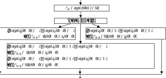
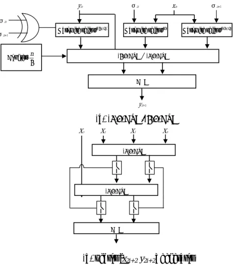
(4) more σ values in each step. Now, the proposed architecture requires two σ values in each step. The σ -value prediction algorithm is described as below: σ 2i is determined by sign of z (2i) , and three equations for determining z(2i+2) are defined as z1 (2i + 2) = z (2i ) − σ 2i (tan −1 2 −2i + tan −1 2 − ( 2i +1) ) (43) z 2 (2i + 2) = z (2i ) − σ 2i (tan −1 2 −2i − tan −1 2 − ( 2i +1) ) (44) z3 (2i + 2) = z (2i ) − σ 2i tan −1 2 −2i (45) The flowchart for the σ 2i +1 -prediction and z (2i + 2) determination algorithm is illustrated in Fig. 2, detailed flowcharts for specific cases are illustrated in Fig. 3 and 4, respectively. Now, the σ 2i +1 -prediction and z (2i + 2) determination algorithm is analyzed and developed, this algorithm is simple and easy to implement on hardware. Thus, the algorithm is very suited to VLSI implementation. The determination circuit of σ 2i +1 and z(2i+2) is shown in Fig. 5. The −1. −2 i. −1. as follows: ⎧⎡ 1 ⎫ − δ 2i 2−2i ⎤⎡U2i ⎤ ⎪⎢ ⎪ ⎥⎢ ⎥ −2i 1 ⎦⎣V2i ⎦ ⎡U2i+1 ⎤ 1 ⎪⎣δ 2i 2 ⎪ ⎬ (46) ⎢V ⎥ = 2 ⎨ − i 2 ⎡ 1 − δ 2i 2 ⎤⎡ X 2i ⎤⎪ ⎣ 2i+1 ⎦ k2i ⎪ −2i ⎥⎢ ⎥ ⎪− ρ2i 2 ⋅ ⎢δ 2−2i 1 ⎦⎣ Y2i ⎦⎪⎭ ⎣ 2i ⎩ 1 W2i +1 = (W2i + ρ 2i 2 −2i Z 2i ) (47) k 2i ⎧⎡ 1 ⎫ − δ 2i 2−2i ⎤⎡ X 2i ⎤ ⎪⎢ ⎪ ⎥⎢ ⎥ −2i 1 ⎦⎣ Y2i ⎦ ⎡ X 2i+1 ⎤ 1 ⎪⎣δ2i 2 ⎪ ⎬ ⎢Y ⎥ = 2 ⎨ −2i k ⎡ 1 − δ 2i 2 ⎤⎡U2i ⎤⎪ ⎣ 2i+1 ⎦ 2i ⎪ −2i ⎥⎢ ⎥ ⎪+ ρ2i 2 ⋅ ⎢δ 2−2i 1 ⎦⎣V2i ⎦⎪⎭ ⎣ 2i ⎩ 1 Z 2i +1 = ( Z 2i − ρ 2i 2 −2i W2i ) k 2i. (48). (49). According to eqs. (46), (47), (48) and (49), we obtain ⎡U 2i + 2 ⎤ 1 − δ 2i +1 2 −2i −1 ⎤ ⎡U 2i +1 ⎤ 1 ⎡ = ⋅ ⎢ ⎥⎢ ⎥ ⎢V ⎥ 2 − 2i −1 1 ⎣ 2i + 2 ⎦ k 2i +1 ⎣δ 2i +1 2 ⎦ ⎣ V2i +1 ⎦ ⎡ 1 − δ 2i+1 2−2i−1 ⎤⎡ X 2i+1 ⎤ 1 − 2 ⋅ ρ2i+1 2−2i−1 ⋅ ⎢ ⎥⎢ ⎥ (50) −2i −1 k2i+1 1 ⎦⎣ Y2i+1 ⎦ ⎣δ 2i+1 2 W2i + 2 =. − ( 2 i +1). series constants of (tan 2 + tan 2 ), −1 −2 i −1 − ( 2 i +1) (tan 2 − tan 2 ) and −1 −2 i (tan 2 ) are stored in ROM and the size 3 of ROM is n words. The accelerated 2 CORDIC architecture with the rotation mode in the circular coordinate system is shown in Fig. 6. In this architecture, the (4,2) carry-save adder (CSA) and carry-propagation adder (CPA) consists of two three-input, and two-output (3,2) carry-save adders/subtractors and one carry-look-ahead adder (CLA).. 1 k 2i +1. (W2i +1 + ρ 2i +1 2 −2i −1 Z 2i +1 ). (51). ⎡ X 2i + 2 ⎤ 1 − δ 2i +1 2 −2i −1 ⎤ ⎡ X 2i +1 ⎤ 1 ⎡ = ⋅ ⎢ ⎥⎢ ⎥ ⎢Y ⎥ 2 − 2i −1 1 ⎣ 2i + 2 ⎦ k 2i +1 ⎣δ 2i +1 2 ⎦ ⎣ Y2i +1 ⎦ ⎡ − δ 2i+1 2−2i−1 ⎤⎡U 2i+1 ⎤ 1 1 + 2 ⋅ ρ2i+1 2−2i−1 ⋅ ⎢ ⎥⎢ ⎥ (52) −2i −1 k2i+1 1 ⎣δ 2i+1 2 ⎦⎣V2i +1 ⎦ 1 Z 2i + 2 = ( Z 2i +1 − ρ 2i +1 2 −2i −1W2i +1 ) (53) k 2i +1. where eqs. (52) and (53) are iteration equations of the 3-D double rotation algorithm. Thus, the 3-D double rotation equations is modified as shown below ⎡ 1 ⋅⎢ − 2i −1 ⎣δ 2i +1 2 − δ 2i 2 −2i ⎤ ⎡U 2i ⎤ ⎥⎢ ⎥ 1 ⎦ ⎣ V2 i ⎦. ⎡U 2i + 2 ⎤ 1 ⎢V ⎥ = 2 2 k ⎣ 2i + 2 ⎦ 2i +1 k 2i. 5. Accelerated 3-D Rotation Using the Double Rotation 2-D CORDIC Algorithm. ⎡ 1 ⎢ − 2i ⎣δ 2i 2. The basic concept of the accelerated 3-D rotation is to reduce the iterations. The double rotation CORDIC algorithm [10] is applied to reduce the iterations or computation time. The 3-D double rotation iteration equations are derived and the computation complexity is also evaluated. The 3-D rotation equations are also written in the form of matrix multiplications. −. ρ 2i ρ 2i +1 ⋅ 2 −4i −1 ⎡ 1 − δ 2i +1 2 −2i −1 ⎤ ⋅ ⎢ ⎥ −2i −1 1 k 22i +1k 22i ⎣δ 2i +1 2 ⎦. ⎡ 1 ⎢ − 2i ⎣δ 2i 2 −. − δ 2i 2 −2i ⎤ ⎡U 2i ⎤ ⎥⎢ ⎥ 1 ⎦ ⎣V2i ⎦. − δ 2i +1 2 −2i −1 ⎤ 1 ρ 2 i ⋅ 2 −2 i ⎡ ⋅ ⎢ ⎥ k 22i +1 k 22i ⎣δ 2i +1 2 − 2i −1 1 ⎦. ⎡ 1 ⎢ − 2i ⎣δ 2i 2. 4. − δ 2i +1 2 −2i −1 ⎤ ⎥ 1 ⎦. − δ 2 i 2 − 2 i ⎤ ⎡ X 2i ⎤ ⎥⎢ ⎥ 1 ⎦ ⎣ Y2i ⎦.

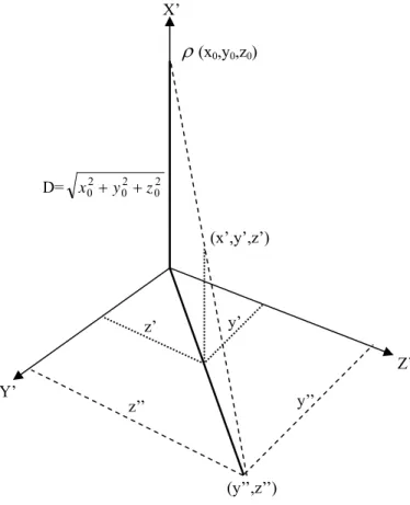
(5) −. − δ 2i +1 2 −2i −1 ⎤ 1 ρ 2i +1 ⋅ 2 −2i −1 ⎡ ⋅ ⎢ ⎥ − 2i −1 k 22i +1 k 22i 1 ⎣δ 2i +1 2 ⎦. ⎡ 1 ⎢ − 2i ⎣δ 2i 2 W2i+2 =. 1 k2i k2i+1 W2i + ρ2i 2 Z2i + ρ2i+1 2 −2i. −2i −1. ⎡ ⎡ X 2i + 2 ⎤ 1 1 ⎢Y ⎥ = 2 2 ⋅ ⎢ − 2i −1 ⎣ 2i + 2 ⎦ k 2i +1 k 2i ⎣δ 2i +1 2 ⎡ 1 − δ 2 i 2 − 2i ⎤ ⎡ X 2i ⎤ ⎢ ⎥⎢ ⎥ − 2i 1 ⎣δ 2i 2 ⎦ ⎣ Y2i ⎦. − δ 2i +1 2 −2i −1 ⎤ ⎥ 1 ⎦. +. +. ρ 2i +1 ⋅ 2 k. 2 2 2 i +1 2i. k. ⎡ 1 ⎢ − 2i ⎣δ 2i 2 Z2i+2 =. ⎡ 1 ⋅⎢ − 2 i −1 ⎣δ 2i +1 2. Z2i+2 =. − δ 2i +1 2 1. −2 i −1. ⎤ ⎥ ⎦. − δ 2i 2 − 2i ⎤ ⎡U 2i ⎤ ⎥⎢ ⎥ 1 ⎦ ⎣ V2i ⎦. 1 . k2ik2i+1. (Z2i − ρ2i ρ2i+12. −4i −1. Z2i − ρ2i 2 W2i − ρ2i+12. (56). −2i −1. W2i ). The additional computation complexity of parallel processing for eqs. (54), (55), (56) and (57) is three additions, one double rotation CORDIC computation and one shit for each iteration. In the n-bit operand n system, when i ≥ − 1 , eqs. (54), (55), (56) 4 and (57) become ⎡ ⎡U 2i + 2 ⎤ 1 1 ⎢V ⎥ = 2 2 ⋅ ⎢ − 2i −1 ⎣ 2i + 2 ⎦ k 2i +1 k 2i ⎣δ 2i +1 2 ⎡ 1 − δ 2i 2 −2i ⎤ ⎡U 2i ⎤ ⎢ ⎥⎢ ⎥ − 2i 1 ⎣δ 2i 2 ⎦ ⎣ V2 i ⎦ −. − δ 2i 2 − 2i ⎤ ⎡U 2i ⎤ ⎥⎢ ⎥ 1 ⎦ ⎣ V2i ⎦. − δ 2i 2 − 2i ⎤ ⎡U 2i ⎤ ⎥⎢ ⎥ 1 ⎦ ⎣ V2i ⎦. 1 (Z2i − ρ2i 2−2i W2i − ρ2i+1 2−2i−1W2i ) k2i k2i+1. (60). (61). 6. 3-D Central Perspective Method Using CORDIC Algorithm. The 3-D central perspective method is shown in Fig. 8 [7]. The graphic is rotated in 3-D space and mapped onto Y’-Z’ plane perspectively. We obtain the coordinate (0, y " , z " ) in Y’-Z’ plane as follows: x" = 0 (62) D y" = ⋅ y' (63) D − x' D (64) z" = ⋅ z' ' D−x. − δ 2i +1 2 −2i −1 ⎤ ⎥ 1 ⎦. − δ 2i +1 2 −2i −1 ⎤ ρ 2 i ⋅ 2 −2 i ⎡ 1 ⋅ ⎢ ⎥ 1 k 22i +1 k 22i ⎣δ 2i +1 2 − 2i −1 ⎦. ⎡ 1 ⎢ − 2i ⎣δ 2i 2. − δ 2i +1 2 −2i −1 ⎤ ⎥ 1 ⎦. Thus, the additional computation complexity of parallel processing is two additions, one double rotation CORDIC computation and one shift for each iteration. The computation time of the double rotation CORDIC algorithm is also reduced [10]. The 3-D rotation with conventional CORDIC algorithm versus the 3-D rotation with double rotation CORDIC algorithm is shown in Fig. 7.. (57) −2i. 1 (W2i + ρ 2i 2 −2i Z 2i + ρ 2i +1 2 −2i −1 Z 2i ) (59) k 2i k 2i +1. − δ 2i +1 2 −2i −1 ⎤ 1 ρ 2i +1 ⋅ 2 −2i −1 ⎡ ⋅⎢ ⎥ − 2 i −1 2 2 1 k 2i +1 k 2i ⎣δ 2i +1 2 ⎦. ⎡ 1 ⎢ − 2i ⎣δ 2i 2. − δ 2i 2 − 2i ⎤ ⎡U 2i ⎤ ⎥⎢ ⎥ 1 ⎦ ⎣ V2i ⎦. (58). − δ 2i +1 2 −2i −1 ⎤ ρ 2i ⋅ 2 −2i ⎡ 1 ⋅ ⎢ ⎥ 1 k 22i +1 k 22i ⎣δ 2i +1 2 − 2i −1 ⎦. ⎡ 1 ⎢ − 2i ⎣δ 2i 2. − δ 2i +1 2 −2i −1 ⎤ ρ 2i ⋅ 2 −2i ⎡ 1 ⋅ ⎢ ⎥ 1 k 22i +1 k 22i ⎣δ 2i +1 2 − 2i −1 ⎦. −2i −1. − δ 2 i 2 − 2 i ⎤ ⎡ X 2i ⎤ ⎥⎢ ⎥ 1 ⎦ ⎣ Y2i ⎦. ⎡ ⎡ X 2i + 2 ⎤ 1 1 ⎢Y ⎥ = 2 2 ⋅ ⎢ − 2i −1 ⎣ 2i + 2 ⎦ k 2i +1 k 2i ⎣δ 2i +1 2 ⎡ 1 − δ 2i 2 − 2 i ⎤ ⎡ X 2i ⎤ ⎢ ⎥⎢ ⎥ − 2i 1 ⎣δ 2i 2 ⎦ ⎣ Y2i ⎦. Z2i ). − δ 2i 2 − 2 i ⎤ ⎡ X 2 i ⎤ ⎥⎢ ⎥ 1 ⎦ ⎣ Y2i ⎦. ⎡ 1 ⎢ − 2i ⎣δ 2i 2 +. W2i +2 =. ρ 2i ρ 2i +1 ⋅ 2 −4i −1 ⎡ 1 − δ 2i +1 2 −2i −1 ⎤ ⋅⎢ ⎥ 2 2 − 2i −1 1 k 2i +1k 2i ⎣δ 2i +1 2 ⎦. ⎡ 1 ⎢ − 2i ⎣δ 2i 2. − δ 2i +1 2 −2i −1 ⎤ 1 ρ 2i +1 ⋅ 2 −2i −1 ⎡ ⋅ ⎢ ⎥ − 2i −1 1 k 22i +1 k 22i ⎣δ 2i +1 2 ⎦. ⎡ 1 ⎢ − 2i ⎣δ 2i 2. (55). (W2i − ρ2i ρ2i+1 2. +. (54). − δ 2 i 2 − 2 i ⎤ ⎡ X 2i ⎤ ⎥⎢ ⎥ 1 ⎦ ⎣ Y2i ⎦. −4i −1. −. −. − δ 2 i 2 − 2 i ⎤ ⎡ X 2i ⎤ ⎥⎢ ⎥ 1 ⎦ ⎣ Y2i ⎦. where D = x02 + y02 + z 02 , ( x0 , y0 , z 0 ) is the 5.

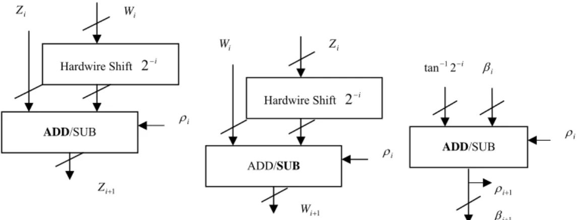
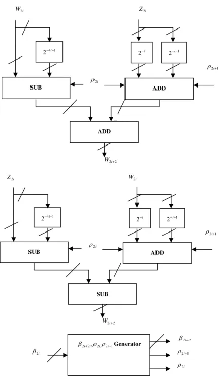
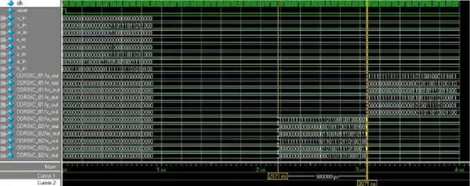
(6) The hardware codes of both that with CORDIC algorithm and double rotation algorithm are written in Verilog-hardware description Language (HDL) [11] running on SUN Blade 1000 workstation under ModelSim simulation tool [12]. Both of two architectures were synthesized by Xilinx FPGA express tools [13] and emulated on the Xilinx XC2V4000 FPGA platform [14]. In the 32-bit accelerated architecture of 3-D rotation, compared with the conventional CORDIC-based architecture of 3-D rotation, the accelerated design improves the latency by more than 30%. The timing diagram for the conventional CORDIC-based architecture and the accelerated architecture of 3-D rotation is shown in Fig. 12. It is designed to evaluate the hardware and to provide an intellectual property (IP) for 3-D graphic engine.. coordinate of observer, and ( x ' , y ' , z ' ) is the rotated coordinate. 7. VLSI Architectures for 3-D Rotation and Perspective with CORDIC Algorithm 7.1 The Architecture of 3-D Rotation with Conventional CORDIC Algorithm. Fig. 9 shows the architecture of the 3-D rotation with the rotation mode in a CORDIC circular coordinate system. In this architecture, the (U i +1 ,Vi +1 ) and ( X i +1 , Yi +1 ) generator each consists of two 2-D CORDIC processors, two hardwire shifts and two adders/subtrators. The Wi +1 and Z i +1 generator each consists of a half of 2-D CORDIC Processor. 7.2 The Architecture of 3-D Rotation with Double Rotation CORDIC Algorithm. 8. Impact of New Architectures and Algorithms. The architecture of the 3-D rotation with double rotation CORDIC algorithm is shown in Fig. 10. In this architecture, the (U i +1 ,Vi +1 ) and ( X i +1 , Yi +1 ) generator each consists of two 2-D CORDIC processors, six hardwire shifts and three adders/subtrators. The Wi +1 and Z i +1 generator each consists of a half of 2-D double rotation CORDIC Processor. The 3-D rotation with double rotation CORDIC algorithm can improve the latency time by more than thirty percent [10].. The Euler angle method consists of sequence of three rotations [2] [6], each rotates one of three orthogonal axes. This method is represented by Euler angles correspond to the sequence of rotations about the coordinate axes. The 3-D rotation method is implemented by cascading two 2-D CORDIC processors [2] [6]. Lang and Antelo proposed a method that replaces two 2-D CORDIC processors by one 3-D CORDIC processor [6]. The sequence of rotations consists of one 2-D CORDIC rotation and one 3-D CORDIC rotation. Both of them require more than two 2-D CORDIC computations. According to the proposed 3-D rotation algorithm, the architecture with conventional CORDIC processors requires one 2-D CORDIC computation in parallelism to perform 3-D rotation, and the architecture with double rotation 2-D CORDIC processors requires less than one 2-D CORDIC computation in parallelism to perform 3-D rotation. The 3-D central perspective method requires four 2-D CORDIC computations in parallelism; this method with CORDIC. 7.3 The Architecture of 3-D perspective Method with CORDIC Algorithm. The proposed architecture of 3-D perspective method consists of five 2-D CORDIC processors and one subtractor. Two CORDIC processors operate in the circular coordinate system for computing x02 + y02 + z 02. ,. and. three. CORDIC. processors operate in the linear coordinate system for computing x " and y " . The architecture of 3-D central perspective method is shown in Fig. 11. 6.

(7) Vol.38, 1971, pp.379-385. [5] O. Mencer, L. Semeria, M. Morf, J. Delosme, “Application of Reconfigurable CORDIC Architecture,” The Journal of VLSI Signal Processing, Special Issue on Reconfigurable Computing, March 2000. [6] T. Lang, E. Antelo, “High-Throughput 3-D Rotations and Normalizations,” Thirty-Fifth Asilomar Conference on Signal, Systems and Computers, 2001, pp.846-851. [7] T. Y. Sung, “Survey of 3-D Perspective Methods for Graphic Engine,” Technical Report (SV-041117), SoC and VLSI Signal Processing Lab., Department of Microelectronics Engineering, Chung Hua University, Hsinchu, Taiwan, 2004. [8] J. Euh, J. Chittamuru, W. Burson, “CORDIC Based Interporator for 3-D Graphics,” IEEE Workshop on Signal Processing Systems, 2002, pp.240-245. [9] S. Wang, E. E. Swartzlander Jr., “Merged CORDIC Algorithm,” Proc. Int’l Symp. Circuits and Systems, 1995, pp.1988-1991. [10] T. Y. Sung, C. S. Chen, M. C. Shih, “The Double Rotation CORDIC Algorithm: New Results for VLSI Implementation of Fast Sine/Cosine Generation,” 2004 International Computer Symposium (ICS-2004), Taipei, Taiwain, Dec. 15-17, 2004. [11] D. E. Thomas, P. H. Moorby, The Verilog Hardware Description Language, Fifth Edition, Kluwer Academic Pub. 2002. [12] Model ModelSim Products: http://www. model.com/products. [13] Synopsys FPGA Express, http://www. synopsys.com/products. [14] Xilinx FPGA products, http://www. xilinx.com/products.. algorithm saves multipliers and square-root, and the implementation of this architecture is required by CORDIC processors only. 9. Conclusions. We have presented two high-throughput 3-D rotation algorithms and architectures both of them are based on 2-D CORDIC algorithm and 2-D double rotation CORDIC algorithm. It is required one or less 2-D CORDIC computation to perform 3-D rotation; and the central perspective method is also performed by 2-D CORDIC algorithm, the architecture of the central perspective method saves hardware and achieves high-performance. The proposed architectures are implemented by 2-D CORDIC processors; the architectures are simple and regular, and suitable for VLSI implementation. The graphic engine should be improved by the proposed algorithms and architectures. 10. References. [1] D. Luebke, M. Reddy, J. D. Cohen, A. Varshney, B. Watson, R. Huebner, “Level of Detail for 3-D Graphics,” Morgan Kaufmann Pub., 2003. [2] D. H. Eberly, “3-D Game Engine Design-A Practical Approach to Real-Time Computer Graphics,” Morgan Kaufmann Pub., 2001. [3] J. E. Volder, “The CORDIC Trigonometric Computing Technique,” IRE Transactions on Electronic Computers, Vol. EC-8, 1959, pp. 330-334. [4] J. S. Walther, “A Unified Algorithm for Elementary Functions,” Spring Joint Computer Conference Proceedings,. 7.

(8) Table 1 Functions of CORDIC arithmetic. System. Rotation Mode z ( n) → 0. Vectoring Mode y ( n) → 0. Linear m=0. x(n) = x(0) y (n) = y (0) + x(0) ⋅ z (0). x ( n ) = x ( 0) y (0) z ( n) = z + x(0). Circular m=1. 1 ( x(0) cos z (0) − y (0) sin z (0)) K1 1 y ( n) = ( y (0) cos z (0) + x(0) sin z (0)) K1. Coordinate. Hyperbolic m=-1. 1 ( x(0) 2 + y (0) 2 ) K1 y (0) z (n) = z (0) − tan −1 ( ) x(0). x ( n) =. x ( n) =. 1 ( x(0) cosh z (0) + y (0) sinh z (0)) K −1 1 y ( n) = ( y (0) cosh z (0) + x(0) sinh z (0)) K −1. x ( n) =. 1 ( x(0) 2 − y (0) 2 ) K −1 y (0) ) z (n) = z (0) + tanh −1 ( x (0). x ( n) =. z. Ri. φi. x. θi y. Fig.1. A vector R in three dimensional space Begin. For ( i = 0; i ≤. n − 1; i + + ) 2. Evaluate. σ 2i = sign( z (2i )) ==1. Yes. Branching. Flowchart in Fig. 2. No. Flowchart in Fig. 3. Fig. 2. Flowchart for the σ 2i +1 -prediction and z (2i + 2) determination algorithm. Detailed flowcharts for specific cases when sign(z(2i)) evaluation returns +1 , -1, and when the algorithm is in a branching are 8.

(9) σ 2i = sign( z (2i)) == +1. Perform in parallel if ( sign( z1 (2i + 2) ="+" ) ∧ ( sign( z2 (2i + 2) ="+" ). if ( sign( z1 (2i + 2) ="−") ∧ ( sign( z2 (2i + 2) ="−"). then σ 2i +1 = +1, z (2i + 2) = z1 (2i + 2). then σ 2i +1 = −1, z (2i + 2) = z2 (2i + 2). if ( sign( z1 (2i + 2) ="−" ) ∧ ( sign( z2 (2i + 2) ="+" ) ∧ ( sign( z3 (2i + 2) ="−" ) then σ 2i +1 = −1, z (2i + 2) = z2 (2i + 2) if ( sign( z1 (2i + 2) ="−" ) ∧ ( sign( z2 (2i + 2) ="+" ) ∧ ( sign( z3 (2i + 2) ="+" ) then σ 2i +1 = +1, z (2i + 2) = z1 (2i + 2). Fig. 3. Flowchart for i-iteration for the case when σ 2i = sign( z (2i)) evaluation returns +1. σ 2i = sign( z (2i)) == −1 Perform in parallel if ( sign( z1 (2i + 2) ="+" ) ∧ ( sign( z2 (2i + 2) ="+" ). if ( sign( z1 (2i + 2) ="−") ∧ ( sign( z2 (2i + 2) ="−"). then σ 2i +1 = +1, z (2i + 2) = z2 (2i + 2). then σ 2i +1 = −1, z (2i + 2) = z1 (2i + 2). if ( sign( z1 (2i + 2) ="+" ) ∧ ( sign( z2 (2i + 2) ="−" ) ∧ ( sign( z3 (2i + 2) ="+" ) then σ 2i +1 = +1, z (2i + 2) = z2 (2i + 2) if ( sign( z1 (2i + 2) ="+" ) ∧ ( sign( z2 (2i + 2) ="−" ) ∧ ( sign( z3 (2i + 2) ="−" ) then σ 2i +1 = −1, z (2i + 2) = z1 (2i + 2). Fig. 4. Flowchart for i-iteration for the case when σ 2i = sign( z (2i)) evaluation returns -1 z(2i+2). z (2i). ± Δ1(2i). Sign(z1(2i+2)) z (2i) Sign(z2(2i+2)). ±. 2：1 Multiplexer. σ2i+1. z2(2i+2). Determination. Sign(z2(2i+2)). (2:1 Multiplexer) σ2i. z (2i) z1(2i+2). σ2i+1. ±. z2(2i+2). (a) Determination circuit of z (2i + 2). z(2i+2). Circuit. Δ2(2i) σ2i. Sign(z1(2i+2)). z1(2i+2). Δ3(2i). (b) σ 2i ,σ 2i+1 and z (2i + 2) generator Fig. 5. The determination circuit of σ 2i , σ 2i +1 and z (2i + 2) 9.

(10) y2i. x2i. σ2i. σ2i+1. σ2i. Hardwire shift 2-(4i+1). σ2i+1. Counter-. n 4. Hardwire shift 2-2i. Hardwire shift 2-(2i+1). (4,2)CSA╱(3,2)CSA. CLA. y2i+2. (a) (3,2)CSA/(4,2)CSA X3. X2. X1. X0. (3,2)CSA. (3,2)CSA. CLA. (b) vector [x2i+2 y2i+2] generator Fig. 6. The accelerated CORDIC architecture with the rotation mode in the circular coordinate system.. Fig. 7 3-D rotation with conventional CORDIC algorithm versus 3-D rotation with double π. π. π. π. 3. 4. 2. 3. rotation CORDIC algorithm ( R0 = 1,α 0 = , β 0 = ,θ 0 = ,φ0 =. 10. ).

(11) X’. ρ (x0,y0,z0). D= x 02 + y 02 + z 02 (x’,y’,z’). y’. z’. Z’ Y’. y’’. z’’. (y’’,z’’). Fig. 8. The 3-D central perspective method Ui. δi. Vi. Xi. αi. Yi. 2-D CORDIC. 2-D CORDIC. δ i +1 Hardwire Shift. ρi Xi. 2. −i. ADD/SUB. Yi. δi. 2. Hardwire Shift. α i +1. −i. ρi. ADD/SUB. Ui. αi. Vi. U i +1. Vi +1. 2-D CORDIC. 2-D CORDIC. δ i +1 Hardwire Shift. ρi. 2 −i. Hardwire Shift. ADD/SUB. 2 −i. ρi. ADD/SUB. X i +1. Yi +1. 11. α i +1.

(12) Zi. Wi Wi. Hardwire Shift. 2. Zi. −i. tan −1 2 − i Hardwire Shift. βi. 2 −i. ρi. ADD/SUB. ADD/SUB. ρi. ADD/SUB. ρi. ρ i+1. Z i+1 Wi +1. β i+1. Fig. 9. The architecture of the 3-D Rotation with 2-D CORDIC algorithm U 2i. V2i. δ 2i. X 2i. Double Rotation CORDIC. 2 −4i −1. α 2i. Y2i. Double Rotation CORDIC. 2 −4i −1. 2 −2i. 2 −2i −1. 2 −2i. δ 2i + 2. 2 −2i −1. α 2i + 2 ρ 2i SUB. ρ 2i +1 ADD. ρ 2i +1. SUB. X 2i. Y2i. δ 2i. U 2i + 2. V2 i + 2 U 2i. Double Rotation CORDIC. 2 −4i −1. α 2i. V2 i. Double Rotation CORDIC. 2 −4i −1. 2 −2i. 2 −2i −1. 2 −2i. δ 2i + 2. 2 −2i −1. α 2i + 2 ρ 2i SUB. ADD. ρ 2i +1. ADD. X 2i + 2. Y2i + 2. 12. ρ 2i +1.

(13) W2 i. Z 2i. 2 −4i −1. 2 −i. 2 −i −1. ρ 2i +1 ρ 2i SUB. ADD. Z 2i ADD. W2 i + 2 Z 2i. W2 i. 2 −4i −1. 2 −i. 2 −i −1. ρ 2i +1. ρ 2i SUB. ADD. SUB. W2 i + 2. β 2i. β 2i + 2 , ρ 2i , ρ 2i +1 Generator. β 2i + 2 ρ 2i +1 ρ 2i. Fig. 10. The architecture of the 3-D Rotation with Double Rotation CORDIC algorithm. 13.

(14) x0. x'. D. 0. y0. 2-D CORDIC. SUB. (Vectoring Mode, Circular Coordinate). 0. D−x. '. 0. z0. 2-D CORDIC (Vectoring Mode, Linear Coordinate) 2-D CORDIC. (Vectoring Mode, Circular Coordinate) D D − x'. D D D − x'. 0. 0. D D' − x ' z. y'. 2-D CORDIC (Rotation Mode, Linear Coordinate). 2-D CORDIC (Rotation Mode, Linear Coordinate). z'' y' '. Fig. 11. The architecture of 3-D central perspective method. Fig. 12. The timing diagram for the conventional CORDIC-based architecture and the accelerated architecture of 3-D rotation (CORDIC_01: Conventional CORDIC, CORDIC 02: Double rotation CORDIC). 14.

(15)