1
A Multi-Class SVM Classification System
Based on Methods of Self-Learning and
Error Filtering
JuiHis Fu
ChihHsiung Huang
SingLing Lee
Department of Computer Science and Information Engineering
National Chung Cheng University
Chiayi 62107, Taiwan, Republic of China
{fjh95p, hch94, singling}@cs.ccu.edu.tw
Abstract—In this paper, the technique of Sup-port Vector Machine has been used to deal with multi-class Chinese text classification. Several data retrieving techniques including word segmentation, term weighting and feature extraction are adopted to implement our system. To improve classification accuracy, two revised methods, self-learning and error filtering, for straight forward SVM results are pro-posed. The method of self-learning uses misclassified documents to retrain classification system, and the method of error filtering filters out possibly misclas-sified documents by analyzing the decision values from SVM. The experiment result on real-world data set shows the accuracy of basic SVM classification system is about 79% and the accuracy of improved SVM classification system can reach 83%.
Index Terms—Document Classification, Support Vector Machine (SVM), Multi-Class SVM, Error Fil-tering
I. INTRODUCTION
With more and more articles and documents in the information system, how to automatically classify information becomes a main research subject. The methods for document classification can be divided into two major types, retrieving semantic meaning of the document content and calculating the statistical similarity of documents. The second type is much popular because the first type is more time-consuming to deal with large set of semantic information. SVM classification system is based on the second approach.
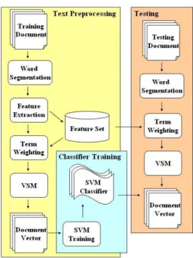
Document classification can be taken into two steps, text preprocessing and classifier training. Figure 1 is an overview of our document classi-fication system. Text preprocessing involves data retrieving techniques, includes segmenting a long sentence to serval shorter terms (word segmenta-tion), eliminating the meaningless keywords (fea-ture extraction), computing the weight of key-words (term weighting), and representing a docu-ment in Vector Space Model (VSM). In feature
ex-Fig. 1. SVM system for Text Preprocessing ,Classifier Training, and Classification.
traction, it computes the weights of all keywords, then eliminates some keywords with weights lower than a predefined threshold. To compute the weight of each keyword, three methods, Term Frequency (TF), Term Frequency * Inverse Docu-ment Frequency (TFIDF), and Information Gain (IG)[6], are adopted in our system. Two normal-ization techniques, L1 and L2 normalnormal-ization[16], are also applied in term weighting to compare the performance difference.
Some well-known classification methods like K-Nearest Neighbors (KNN)[15], Support Vector Machines (SVM)[5][3][7], Naive Bayes[10], and neural network[14] have been well studied re-cently. We chooses SVM as our basic classifier
because SVM has been proven very effective in many research results and is able to deal with large dimensions of feature space. SVM is a statis-tic classification method proposed by Cortes and Vapnik in 1995 [7]. It is originally designed for binary classification. The derived version, a multi-class SVM, is a set of binary SVM multi-classifiers able to classify a document to a specific class.
In addiction to use the basic classification tech-niques, we propose two revised methods, self-learning and error filtering, to increase the accu-racy of multi-class SVM classification. The idea of these two methods is as follows:
1) The method of self-learning
The classifier will retrain itself by combining the original training set and the misclassi-fied documents to a new training set. This method avoids misclassifying similar docu-ments again.
2) The method of error filtering
The system will identify documents which are difficult to be differentiated from all classes. If a document is marked as ”indis-tinct”, it means the document has high prob-ability to be misclassified. To avoid misclas-sifying, the document should be reclassified by other classification methods.
Our experiment uses 6000 official documents of the National Chung Cheng University from the year 2002 to 2005. These documents have a commonly special property that there are seldom words in their contents. The average number of keywords in each document is nearly 10. This leads to a challenge on the accuracy of the classi-fication system. In order to compare performance, our experiment implements several data retriev-ing techniques, TF, TFIDF, and IG as the feature extraction scheme and TF, TFIDF with L1 and L2 normalization as the term weighting scheme. We also adjust the filtering level of feature extraction to find out the best strategy. The filtering level is a percentage threshold of feature extraction. The experiment shows the best strategy is to take IG with filtering level 0.9 as the scheme of fea-ture extraction and TFIDF with L2 normalization as the scheme of term weighting. The accuracy is about 79.83%. When adopting the method of self-learning, the average accuracy raises 1.64%. Adopting the method of error filtering, the aver-age accuracy is up 4.45%. Combining the methods of self-learning and error filtering, the average accuracy improves 5.54% higher.
The rest of the paper is organized as follows: Chapter 2 briefly introduces some multi-class SVM classifications. Chapter 3 presents the pro-cedure of the classification system in this work. Chapter 4 presents the two methods of self-learning and error filtering. Chapter 5 shows the
experiment performance of the classification sys-tem. Chapter 6 summarizes the main idea of this paper.
II. RELATED WORKS
The first process of classifying documents is to weight terms in documents. There are several popular methods like Mutual Information (MI), Chi Square Statistic (CHI), Term Frequency * Inverse Document Frequency (TFIDF), Information Gain (IG), etc. Based on these weights, it’s easier to decide which terms are significant and which terms should be filtered. Then, our classification procedure is to represent documents in Vector Space Model (VSM) and classify vectors by SVM classifier.
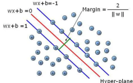
Support Vector Machine (SVM) is a statistical classification system proposed by Cortes and Vap-nik in 1995[7]. The simplest SVM is a binary classifier, which is mapping to a class and can identify an instance belonging to the class or not. To produce a SVM classifier for class C, the SVM must be given a set of training samples including positive and negative samples. Positive samples belong to C and negative samples do not. After text preprocessing, all samples can be translated to n-dimensional vectors. SVM tries to find a separating hyper-plane with maximum margin to separate the positive and negative examples from the training samples.
Fig. 2. Support vector machine
There are two kinds of multi-class SVM system[5], all(OAA) and one-against-one(OAO). The OAA SVM must train k binary SVMs where k is the number of classes. The
ith SVM is trained with all samples belonging
to ith class as positive samples, and takes other examples to be negative samples. These k SVMs could be trained in this way, and then k decision functions are generated. After setting up all SVMs with positive and negative samples, it trains all
k SVMs. Then it can get k decision functions.
For a testing data, we compute all the decision values by all decision functions and choose the
maximum value and the corresponding class to be its resulting class.
The class of input data x = arg max
i=1...k(wi· x + b) The OAO SVM is that for every combination of two classes i and j, it must train a corresponding
SV Mij. Therefore, it will train k(k − 1)/2 SVMs and get k(k−1)/2 decision functions. For an input data, we compute all the decision values and use a voting strategy to decide which class it belongs to. If sign(wij · x + bij) shows x belongs to ith class, then the vote for the ith class is added by one. Otherwise, the jth class is added by one. Finally, x is predicted to be the class with the largest vote. This strategy is also called the “Max Wins” method.
There is no theoretic proof that which kind of multi-class SVM is better, and they are often compared by experiment. In [5][16], it shows the average accuracy of OAA SVM is better than the OAO SVM.
There are some researches for multi-class SVM classification. In [16], it presents a new algorithm to deal with noisy training data, which combines multi-class SVM and KNN method. The result shows that this algorithm can greatly reduce the influence of noisy data on SVM classifier. In [9], it compares OAO SVM, OAA SVM, DAG SVM (Directed Acyclic Graph SVM), and two all to-gether SVM. An all toto-gether SVM means it trains a SVM classifier by solving a single optimization problem. Experiments show that OAO and DAG method may be more suitable for practical use. In [8], it reduces training data by using KNN method before the procedure of SVM classification. The mean idea is to speed up the training time. The experiment compares OAO SVM, DAG SVM, and the proposed hybrid SVM. It shows the accuracy are similar for three methods but the training time of hybrid SVM outperforms the other two methods. In [12], it compares SVM and Naive Bayes in multi-class classification. They both use a method, called ”error correcting output code (ECOC)”, to decide the class label of input data. The experiment shows the accuracy of SVM is better than Naive Bayes method.
III. CLASSIFICATION SYSTEM
A classification system is composed of three phases, Text preprocessing, SVM training, and Performance testing.
• Text preprocessing. Text preprocessing is taken into three steps, Word segmentation, Feature extraction, and Term weighting.
1) Word segmentation. Sentences in docu-ments should be segmented to several
shorter terms. Especially, it’s much dif-ficult to segment Chinese sentence cause there is no natural delimiter be-tween Chinese words. In our implemen-tation, we adopt a Chinese word seg-mentation tool [18], developed by Insti-tute of Information Science in Academia Sinica. It’s obvious that the result of Chinese word segmentation has large influence on accuracy of classification systems.
2) Feature extraction. The following meth-ods are compared experimentally in our system.
– TF, the weight of term i is defined as
w(ti) = tfi , where tfi is the number of occurrences of the ith term.
– TFIDF, w(ti) = tfi× logNni , N is the number of all documents, ni is the number of documents where term i occurs. – Information Gain, w(ti) = − m X j=1 p(cj) log p(cj) +p(ti) m X j=1 p(cj|ti) log p(cj|ti) +p(bti) m X j=1 p(cj|bti) log p(cj|bti) (1)
p(cj) is the probability that terms oc-cur in category j, p(ti) is the prob-ability that term i occurs, p(cj|ti) is the probability that term i occurs in category j, p(bti) is the probability that term i does not occur, p(cj|bti) is the probability that the term i doesn’t occur in category j.
It is difficult to define the threshold for the three methods. We use a percentage threshold instead, named filtering level (F L). Assume n is the number of key-words, let 0 < F L ≤ 1, then it reserves (n ∗ F L) keywords and eliminates the others. The remaining keywords are fea-tures and we use them to represent doc-ument vector. To simplify the notation, we use TFIDF0.8 to denote the TFIDF
with filtering level 0.8.
3) Term weighting. We compared 2 weight-ing methods with 2 normalization meth-ods. – TF with L1 normalization (TFL1), d =(tf1 S , tf2 S , ... , tfn S ), where tfi is the
number of occurrences of the ith term and S =Pni=1ti.
– TF with L2 normalization (TFL2),
d =(tf1
S , tfS2, ... , tfSn), where tfi is the number of occurrences of the ith term and S =pPni=1tf2
i.
– TFIDF with L1 normalization (TFIDFL1), d =(vS1, vS2, ... , vSn), where vi= tfi× lognNi , N is the total number of documents in training set,
ni is the number of documents in training set where term i occurs, and
S =Pni=1tfi× lognNi.
– TFIDF with L2 normalization (TFIDFL2), d =(vS1, vS2, ... , vSn), where vi= tfi× lognNi , N is the total number of documents in training set,
ni is the number of documents in training set where term i occurs, and
S =qPni=1(tfi× lognNi)2.
• SVM training. The OAA SVM is chosen to be our classification system, that is k binary SVMs will be trained and predict the class label of an input data with the maximum decision value. Considering the performance of SVM, a SVM tool, SVMlight[17], developed by Thorsten Joachims, is adopted.
In SVM training, all training data are sepa-rated at first. For example, in figure 3, there are six documents in the training set. Docu-ment a1 belongs to class A, docuDocu-ment b1 and
b2 belong to class B, and document c1, c2, and c3 belong to class C. For the SVM classifier
in C, a1 is in the positive set and other five documents belong to the negative set. For the SVM classifier in B, b1 and b2 are in the pos-itive set and other four documents belong to the negative set. For the SVM classifier in C,
c1, c2, and c3 are in the positive set and other
three documents belong to the negative set. Then SVMlightis executed to train SVM A,B, and C and outputs three trained SVMs. We use the trained SVMs to classify documents.
Fig. 3. Set up training set
• Performance testing. After all classifiers are trained, our system could predict the class label, the class in which the SVM classifier
generates the maximum decision value, of the input data. For a set of testing data, the way to evaluate accuracy is defined as
accuracy =number of correctly classified documents number of total documents
(2)
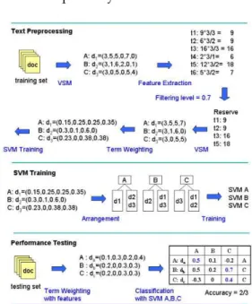
• An example of system flow.
Fig. 4. An example of system flow
Figure 4 is an example of system flow. At first, it needs a training set. Assume there are three documents d1, d2, and d3, and they
belong to classes A, B, and C, respectively. 1) Text preprocessing. Long sentences
should be segmented to shorter terms. The Chinese word segmentation system [18] is used in our implementation. Assume there are six keywords (t1, t2,
..., t6) after word segmentation in our
example. Then A : d1 = (3, 5, 5, 0, 7, 0)
means d1 belongs to class A and
contains 3 term t1, 5 term t2, 5 term t3 and 7 term t5. It uses TFIDF of
feature extraction with filtering level 0.7 (TFIDF0.7). The weight of t
1 is
(3 + 3 + 3) × 3
3 = 9, the weight of t2 is
(5 + 1 + 0) × 3
2 = 9, and so on. Using
the filtering level, 6 × 0.7 = 4.2 ' 4 keywords will be reserved. After feature extraction, it reserves t1, t2, t3 and t5.
Then TF with L1 normalization (TFL1) of term weighting is adopted. For example, the weight of t1 in d1 is
3
3+5+5+7 = 0.15.
2) SVM training. The positive and negative samples for all SVMs should be sep-arated. For example, SVM A takes all samples of class A, d1, to be positive
set and all other samples, d2 and d3,
to be negative set. Then we use the SVMlight[17] tool to be our classification system.
3) Performance testing. Assume there are three testing documents, da, db, and dc, belonging to class A, B, and C, respec-tively. After the procedure of Text pre-processing, these three documents could be classified by all trained SVMs and calculated decision values. Our classi-fication system predicts the class label, the class in which the SVM classifier generate the maximum decision value, of the document. In our example, the decision values are given arbitrarily and the accuracy is 66.67%.
IV. THE IMPROVEMENT OF SYSTEM A. The method of self-learning
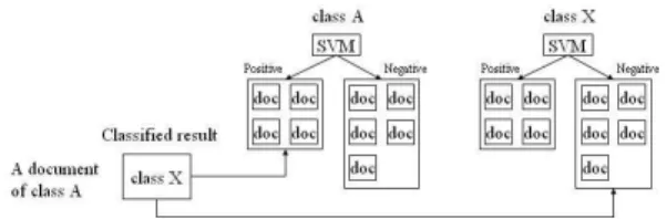
If the class labels of testing data are verified, the system can learn from these data. Not all input data are suitable to retrain system, specific mis-classified data could be taken into consideration. After retraining the system by misclassified data, it would probably not misclassify the similar data. This method is called “Learning from Misclassi-fied Data (LMD)”. The following describes the LMD.
1) Verifying all classified data.
2) For each misclassified data of class A and its predicted class X, showed in figure 5, adding it to the positive set of the SVM in class A and adding to the negative set of the SVM in class X.
3) Retraining these two SVMs in which the training set has been modified.
That is a easy concept, and indeed it can effec-tively increase the accuracy of the system.
Fig. 5. Learning from Misclassified Data (LMD)
B. The method of error filtering
Our classification system chooses the class la-bel, the class in which the SVM generates the maximum decision value, of the input data. But all those decision values could be negative. It means the input data does not belong to any class. It probably leads to misclassification. In the
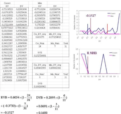
other case, the maximum and second maximum values could be very close. It means the input data is hard to be differentiated from the two most possible classes. It also leads to misclassification. To avoid above situations, we define two vari-ables and two thresholds for decision values. Result Value(RV) is the maximum decision value which means how close the input data is to the predicted class. Difference Value(DV) is the dif-ference between maximum and second maximum value which means how the input data can be clearly separated from two most possible classes.
Fig. 6. The distribution of RV of documents
In figure 6, the x-axis is RV of documents and the y-axis is the number of documents. The solid line is the average RV distribution of correctly classified documents. The dotted line is the av-erage RV distribution of misclassified documents. We can find that if a RV is larger than 0, the threshold, the input data has lots of probability belonging to the corresponding class and we re-turn the class straightforward in our method. The threshold is named “RV bound” (RVB). If the RV is smaller than RVB, we use DV to differentiate the document.
Fig. 7. The distribution of DVs of documents which RVs are smaller than RVB
In figure 7, it is showed the DV distribution of documents with RVs smaller than RVB. In our
method, if the DV is bigger than a threshold, named “Difference Value bound” (DVB), the system will predict the class label of the testing data, or a indistinguishable message otherwise.
An input document is either distinguish-able or indistinguishdistinguish-able. (a) Distinguishable 1) RV ≥ RVB 2) RV < RVB and DV ≥ DVB (b) Indistinguishable 1) RV < RVB and DV < DVB
Now the problem is how to define the two thresholds, RVB and DVB. For the binary classifier in each class, RVB and DVB are individually decided by learning from training data. For a class A and all documents which are classified to class A, the RVB is computed by following formulation
RV B = Cor RV Avg × (1 −Cor N um T otal ) +M is RV Avg × (1 −M is N um
T otal ) (3)
where Cor RV Avg is the average RV of cor-rectly classified data, Cor N um is the number of correctly classified data, M is RV Avg is the average RV of misclassified data, M is N um is the number of misclassified data, and T otal =
Cor N um + M is N um. After determining the
RVB, we compute DVB by documents with RVs smaller than RVB. The formulation is defined as
DV B = Cor DV Avg × (1 −Cor N um
0
T otal0 )
+M is DV Avg × (1 −M is N um
0
T otal0 ) (4) where Cor DV Avg is the average DV of cor-rectly classified data, Cor N um0 is the number of correctly classified data, M is DV Avg is the average DV of misclassified data, M is N um0 is the number of misclassified data, and T otal0 =
Cor N um0+ M is N um0.
The RVB and the DVB will clearly separate the correctly classified and misclassified data. Figure 8 is an example of computing RVB and DVB. The left two columns is the RV and DV of correctly classified data. The right two columns is the RV and DV of misclassified data. The RVB and DVB can be calculated by the two formulations.
C. Combining self-learning and error filtering
In section IV, a method of self-learning, LMD is proposed. LMD chooses the misclassified data to retrain the system. But through separating indistinguishable data from the classified data, there is one strategy to choose which data to
Fig. 8. An example of computing RVB and DVB
retrain the system. Because the predicted class label of some indistinguishable data are correct, they worth to be learned. The indistinguishable data and misclassified data are used to retrain the system, called “Learning from Misclassified and Indistinguishable Data (LMID)”. The following describes the LMID.
1) Varifying all classified data.
2) For each misclassified data with the correct class label A and the predicted class label X, the dotted line in figure 9, adding it to the positive set of the SVM in class A and to the negative set of the SVM in class X.
3) For each indistinguishable data with the correct class label A and the predicted class label A, the solid line in figure 9, adding it to the positive set of the SVM in class A. 4) Retraining the SVMs which training set has
been modified.
The only difference between LMD and LMID is the step 3 in LMID. LMD and LMID are compared experimentally in section V.
V. EXPERIMENT RESULTS
The experiment uses the official documents of the National Chung Cheng University from the year 2002 to 2005. We take 20 units (classes), 150 documents for each unit (class) as training data, and 150 documents for each unit (class) as testing data. Totally we have 6000 documents for experiment. There is a common characteristic among official documents, seldom words in the contents. The average number of keywords in
Fig. 9. Learning from Misclassified and Indistinguishable Data (LMID).
each document is nearly 10. That leads to a chal-lenge on the accuracy of the classification system.
The way to evaluate accuracy is defined as
accuracy =number of correctly classified documents number of total documents
Fig. 10. he accuracy of TF, TFIDF, and IG of feature extraction with TFL2of term weighting
Fig. 11. The accuracy of TF, TFIDF, and IG of feature extraction with TFIDFL2of term weighting
Figure 10 is the result of using TFL2 as term weighting scheme and three kinds of feature ex-traction with increasing filtering level from 0 to 1. Figure 11 is the result of using TFIDFL2 as term weighting scheme. We can find out the IG is better than TFIDF and TF when the filtering level is decreasing but the differentiation is not
so obvious because of the characteristic of seldom words in document content.
Then we compare TFL1, TFL2, TFIDFL1, and TFIDFL2 as term weighting scheme.
Fig. 12. TFL1, TFL2, TFIDFL1, and TFIDFL2of term
weight-ing with TF of feature extraction
Fig. 13. TFL1, TFL2, TFIDFL1, and TFIDFL2of term
weight-ing with TFIDF of feature extraction
Fig. 14. TFL1, TFL2, TFIDFL1, and TFIDFL2of term
weight-ing with IG of feature extraction
Figure 12, 13, and 14 are the results of compar-ing TFL1, TFL2, TFIDFL1, and TFIDFL2 as term weighting scheme with TF, TFIDF, and IG as feature extraction scheme. It is observed TFIDFL2 outperforms the others. In our experiment, we found the best strategy of our classification sys-tem for the input data is IG0.9as feature extraction
scheme with TFIDFL2 as term weighting scheme, and the accuracy of classification is 79.83%.
Table II is the result of using self-learning (LMD) method mentioned in section IV-A. The
Basic SVM LMD SVM Data set Accuracy Accuracy
T1 – – T2 0.7817 0.79 T3 0.785 0.8017 T4 0.77 0.7883 T5 0.8017 0.81 Average 0.7846 0.7975 TABLE I
THE ACCURACY OF USING THE METHOD OF SELF-LEARNING
(LMD) Accuracy Basic SVM EF SVM T1 0.8 0.8263 T2 0.7817 0.8109 T3 0.785 0.8185 T4 0.77 0.7996 T5 0.8017 0.8272 Average 0.78168 0.8165 TABLE II
THE ACCURACY OF USING THE METHOD OF ERROR FILTERING
(EF)
testing data are divided into 5 sets. For each class,there are 30 documents belonging to each set. Totally there are 600 document in each set. We compare results with basic SVM and LMD SVM. Here we use the TFIDFL2as term weighting scheme and TF1.0 as feature extraction scheme.
After classifying each testing data set, the system will automatically be retrianed by itself. There-fore, beside of T1, the other testing sets will have different accuracy. We can find the average accuracy of LMD SVM is better than basic SVM and is 1.64% improvement on accuracy.
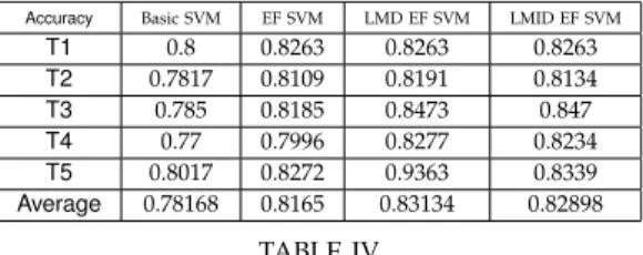
Table IV-C and Table IV-C are the results of using error filtering(EF) method mentioned in section IV-B. We compare the “Basic SVM” and “EF SVM”, they show the average accuracy of “Basic SVM” is 78.168% and “EF SVM” is 81.65% with 94.634% distinguish ability. We can find that “EF SVM” has 4.45% improvement on average accuracy.
Table IV-C and IV-C show the result of using the methods of combining error filtering and self-learning, which is mentioned in section IV-C. It is found that both accuracy and distinguish ability are arising. LMD SVM and LMID SVM has
Distinguish ability EF SVM T1 0.95 T2 0.9517 T3 0.9367 T4 0.0.9483 T5 0.945 Average 0.94634 TABLE III
THE DISTINGUISH ABILITY OF USING THE METHOD OF ERROR FILTERING(EF)
Accuracy Basic SVM EF SVM LMD EF SVM LMID EF SVM
T1 0.8 0.8263 0.8263 0.8263 T2 0.7817 0.8109 0.8191 0.8134 T3 0.785 0.8185 0.8473 0.847 T4 0.77 0.7996 0.8277 0.8234 T5 0.8017 0.8272 0.9363 0.8339 Average 0.78168 0.8165 0.83134 0.82898 TABLE IV
THE ACCURACY OF USING THE METHOD OF COMBINING SELF-LEARNING AND ERROR FILTERING
Distinguish ability EF SVM LMD EF SVM LMID EF SVM
T1 0.95 0.95 0.95 T2 0.9517 0.94 0.467 T3 0.9367 0.9167 0.915 T4 0.9483 0.9383 0.9483 T5 0.945 0.9467 0.9533 Average 0.94634 0.93834 0.94266 TABLE V
THE DISTINGUISH ABILITY OF USING THE METHOD OF COMBINING SELF-LEARNING AND ERROR FILTERING
5.54% and 5.24% improvement, respectively. The accuracy of LMD is better than LMID SVM but LMID SVM has higher distinguish ability.
VI. CONCLUSION
In this paper, soem data retrieving techniques and multi-class SVM classifiers are introduced. After the procedure of Text preprocessing and SVM training, a classification system could be built and then automatically classify documents. Our experiment shows the best strategy is to adopt IG0.9 as feature extraction scheme with
TFIDFL2as term weighting scheme, and the accu-racy of classification is 79.83%. The influence on feature extraction is not obvious because of the characteristic of document contents, few words on average. In order to improve the accuracy of the system, we propose two methods, self-learning and error filtering. In self learning (LMD), it is ob-served that the accuracy of LMD SVM has 1.64% improvement compared to the basic SVM. In error filtering (EF SVM), there is 4.45% improvement on average accuracy . After combining the methods of self-learning and error filtering, the experiment shows the accuracy of LMD and LMID has 5.54% and 5.24% improvement, respectively.
VII. FUTURE WORKS
There are still many other ways to implement feature extraction. We can apply some new meth-ods to the system and compare their experimental results. In section III, there is a short description on word segmentation. Chinese word segmenta-tion is difficult to deal with, and there still is room to improve the influence of word segmentation. After filtering out possibly misclassified data, our classification system does not deal with them. We will figure out other classification methods which
are good at these kind of data in order to improve the accuracy and distinguish ability.
REFERENCES
[1] Bernd Heisele, Purdy Ho, and Tomaso Pog-gio, ”Face Recognition with Support Vector Machines: Global versus Component-based Approach”, IEEE International Conference on Computer Vision, Vol. 2, pp.688-394, 2001. [2] Irene Diaz, Jose Ranilla, Elena Montanes,
Javier Fernandez, and Elias F. Combarro, ”Im-proving Performance of Text Categorization by Combining Filtering and Support Vector Machines”, Journal of the American society for information science and technology, Vol. 55(7), pp.579-542, 2004.
[3] Nello Cristianini and John Shawe-Taylor, ”An Introduction to Support Vector Machines and other kernel-based learning methods”, Cam-bridge University Press, 2000.
[4] Elias F. Combarro, Elena Montanes, Irene Diaz, Jose Ranilla, and Ricardo Mones, ”Intro-ducing a Family of Linear Measures for Fea-ture Selection in Text Categorization”, IEEE Transaction on Knowledge and Data Engi-neering, vol. 17(9), pp.1223-1232, 2005. [5] Jiu-Zhen Liang, ”SVM multi-classifier and
web document classification”, International Conference on Machine Learning and Cyber-netics, Vol.3 , pp.1347-1351, 2004.
[6] Yiming Yang and Jan O. Pedersem, ”A Com-parative Study on Feature Selection in Text Categorization”, International Conference on Machine Learning, pp.412-420, 1997.
[7] C. Cortes and V. Vapnik, ”Support vector net-works”, Machine learning, Vol. 20(3), pp.273-297, 1995.
[8] Fu Chang, Chin-Chin Lin, and Chun-Jen Chen, ”A Hybrid Method for Multiclass Clas-sification and Its Application to Handwritten Character Recognition”, Institute of Informa-tion Science, Academia Sinica, Taipei, Taiwan, Tech. Rep. TR-IIS-04-016, 2004.
[9] Chih-Wei Hsu and Chih-Jen Lin, ”A Compar-ison of Methods for Multiclass Support Vector Machines”, IEEE Transaction on Neural Net-works, vol. 13(2), pp.425-425, 2002.
[10] D. D. Lewis, ”Naive (Bayers) at forty: The independence assumption in information re-trieval”, European Conference on Machine Learning, pp.4-15 , 1998.
[11] Andrew Moore, ”Statistical Data Mining Tu-torials”, http://www.autonlab.org/tutorials/ [12] Jason D. M. Rennie and Ryan Rifkin, ”Im-proving Multiclass Text Classification with the Support Vector Machine”, Massachusetts Institute of Technology, Artificial Intelligence Laboratory Publications, AIM-2001-026, 2001.
[13] G. Salton and C. Buckley, ”Term weighting approaches in automatic text retrieval”, In-formation Processing and Management, Vol. 24(5), pp.513-523, 1988.
[14] E Wiener, ”A neural network approach to topic spotting”, Symposium on Document Analysis and Information Retrieval, pp. 317-332, 1995.
[15] Fang Yuan, Liu Yang, and Ge Yu, ”Improving The K-NN and Applying it to Chinese Text Classification”, International Conference on Machine Learning and Cybernetics, Vol. 3, pp. 1547-1553, 2005.
[16] Jia-qi Zou, Guo-long Chen, and Wen-zhong Guo, ”Chinese Web Page Classification Us-ing Noise-tolerant support vector Machines”, IEEE International Conference on Natural Language Processing and Knowledge Engi-neering, pp.785-790 , 2005.
[17] SVMlight, http://svmlight.joachims.org/ [18] The Chinese Knowledge and Information
Processing (CKIP) of Academia Sinica of Tai-wan, A Chinese word segmentation system, http://ckipsvr.iis.sinica.edu.tw/