在多服務無線網路下提供最佳允入控制

全文

(1)國立交通大學電信工程學系碩士班碩士論文. 在多服務無線網路下提供最佳允入控制. Optimization on Call Admission Control in Multiple-Service Wireless Networks. 研究生：劉政澤指導教授：廖維國. 博士. 中華民國九十三年六月.

(2) 在多服務無線網路下提供最佳允入控制研究生：劉政澤. 指導教授：廖維國博士. 國立交通大學電信工程學系碩士班民國 93 年 6 月. 中文摘要. 隨著第三代行動電話系統的誕生，伴隨的高傳輸速率可提供使用者不同的服務。在無線資源「有限」的情況下，要如何分配頻寬給不同使用者是有趣的，也是允入控制的範疇。在論文中我們假設所關心的是如何讓網路的成本消耗達到最小，該如何做最好的判斷？我們使用馬可夫鏈來模擬頻道的使用狀態，在馬可夫決策過程中尋找最佳策略，也就是根據當時頻寬使用情況和使用者的行為來對新進者做允入判斷。在單一服務下的最佳策略稱為「護衛頻道決策」，我們將修改此策略到多服務的系統下。最終將利用此策略進行一步的「策略改進」，此改進的策略便會是很接近最佳化的策略。. i.

(3) Optimization on Call Admission Control in Multiple-Service Wireless Networks Student: Cheng-Tse Liu. Advisor: Wei-Kuo Liao. INSTITUTE OF COMMUNICATION ENGINEERING NATIONAL CHIAO TUNG UNIVERSITY June, 2004. ABSTRACT With the third-generation mobile phone system coming, it provides multiple-service by higher transmission rate. Since wireless resources are limited, how to allocate the bandwidth is interesting. That is, call admission control is considerable. If we want to minimize the system cost, what can we do? In this thesis, we model channels by Markov chains and find the optimal policy based on Markov decision process. In single service network, the Guard Channel policy is the optimal policy. We will modify it for multiple-service networks, then use this policy to do one-step policy improvement. The next policy is near to the optimal policy.. ii.

(4) 誌謝在研究所的求學過程中，相當感謝廖維國老師對我的指導，老師深厚的知識背景與自由開明的領導都令我深感慶幸。實驗室美好的相處也令我難忘，施邦欣學長、永瑋學長、家宏學長、阿中、怡翔、國瑋、伯谷、于彰、憲良、小智、賢宗，如此完美組合才成為一個活潑的實驗室。最感謝莫過於一路栽培我的父母，有你們的照顧與扶持才有現在的我。陪我長大的大哥與小妹讓我的生活有趣許多，也特別感謝巧雯的陪伴。. iii.

(5) Contents Ⅴ Ⅵ. List of Table List of Figures. Chapter 1: Introduction……………………………………………………….1 Chapter 2: MDP_Based Call Admission Control in Multi-Service Network…………………………….………………………….4 2.1 Multi-rate loss channel model………………………………………..4 2.2 Alternatives (action) and costs……………………………………….6 2.3 The policy-iteration method…………………………………………..7 2.3.1 The value-determination operation…………………………………………..7 2.3.2 The policy-improvement routine……………………………………………10 2.3.3 The one-step policy improvement………………………………….……….11. 2.4 The Guard Channel Policy in Single-Service network……………14 Chapter 3: Evaluation for the Relative Cost in Detail……….………...16 3.1 The Dedicated bandwidth Policy ( π 0 )……………………………16 3.1.1 Cost function in region Ⅰ……………………………………………………………..19 3.1.2 Cost function in region Ⅱ……………………………………………………………..21 3.1.3 Cost function in region Ⅲ……………………………………………………………..24 3.1.4 Cost function in region Ⅳ……………………………………………………………..26 3.1.5 Service bandwidth allocation………………………………………………………….29. 3.2 The Guard Channel Policy ( π 0′ )…………………………………….30 3.2.1 Cost function in region Ⅰ……………………………………………………………..32 3.2.2 Cost function in region Ⅱ……………………………………………………………..34 3.2.3 Service bandwidth allocation………………………………………………………….36. Chapter 4: Numerical Results………………………………………………37 Chapter 5: Conclusion………………………………………………………47 Reference………………………………………………………………………48. iv.

(6) List of Table 4.1 performances of three kinds of policy……………………………………45. v.

(7) List of Figures 2.1 Transition diagram………………………………………………………….5 2.2 Transition diagram with alternative 1 and 2………………………….......6 2.3 The iteration cycle……………………………………………………….12 2.4 LCCM flow diagram……………………………………………………….12 2.5 State transition diagram (Guard Channel Scheme)……………………15 3.1 State transitions in region Ⅰ………………………………………….....19 3.2 State transitions in region Ⅱ……………………………………………21 3.3 State transitions in region Ⅲ……………………………………………24 3.4 State transitions in region Ⅳ……………………………………………27 3.5 State transitions in region Ⅰ for type-1 and type-2 calls……………32 4.1 Channel cost ∆1 (⋅,⋅, n3 = 0, n 4 = 0) …………………………………..……38 4.2 Channel cost ∆1 (⋅, n2 = 0,⋅, n4 = 0) ………………………………….……38 4.3 Channel cost ∆ 2 (⋅,⋅, n3 = 0, n4 = 0) ………………………………….……39 4.4 4.5 4.6 4.7. Channel cost Channel cost Channel cost Channel cost. ∆ 2 (n1 = 0,⋅,⋅, n4 = 0) …………………………………..……39 ∆ 3 (⋅, n 2 = 0,⋅, n 4 = 0) ………………………………….……40 ∆ 3 (n1 = 0, n2 = 0,⋅,⋅) …………………………………..……40 ∆ 4 (⋅, n 2 = 0, n3 = 0,⋅) ………………………………….……41. 4.8 Channel cost ∆ 4 (n1 = 0, n2 = 0,⋅,⋅) …………………………………..……41 4.9 Channel cost ∆ 1′ (n1 + n 2 , n3 + n4 ) …………………………………..…….43 4.10 Channel cost ∆ ′2 (n1 + n 2 , n3 + n 4 ) ………………………………………43 4.11 Channel cost ∆ ′3 (n1 + n2 , n3 + n4 ) ……………………………….……...44 4.12 Channel cost ∆′4 (n1 + n2 , n3 + n4 ) ……………………………….………44. vi.

(8) Chapter 1 Introduction In recent years, there have been tremendous developments and interests in the field of cellular communication. Unlike the old second generation cellular communication systems which only target at voice service provisioning, nowadays the third generation mobile phone systems are capable of providing multiple services, such as conversational real-time audio and video communications. It is believed that an efficient radio resource management scheme to handle such multiplicity is the key to success of the third generation mobile phone system. One of the key issues in radio resource management is the call admission control due to that the wireless resources are much rarer than the wired ones. Therefore, a good admission control scheme for the cellular system with multiple services is to allocate the bandwidth according to the type of the call while the revenue generated by the wireless system can be maximized. With certain reasonable assumptions, the guard channel admission control scheme, which reserves certain amount of bandwidth only for handover calls, is proved to be optimal and practical for the cellular system with the single service. However, as shown in [3,4], the admission control of the multiple services, even in the wired system, is difficult and the optimal solution is computation prohibitive. Therefore, obtaining a near-optimal strategy is what we can expect in attacking the issue of admission control for the cellular system with multiple-service provisioning. To this end, we propose the call admission control scheme called Least Cost Control in Multi-Service wireless networks (LCCM). It is based on the cost function, derived from the context of Markov decision theory [1]. In the general speaking, our proposal is combining the Guard Channel admission control and the Least Cost Routing in Multi-Service Networks. 1.

(9) (LCRM) [3,4] for the multi-service wired networks. Basically, LCRM first models the routing into a Markov decision process (MDP) and uses one-step policy-improvement on a suggested base policy. The novelty of LCRM is in reducing the computation effort to deduce the Howard relative cost function which is mandatory in the policy improvement routing [pp. 37, 1]. In applying LCRM to wireless network, we first note that the call type in the cellular system with single service should be distinguished into “new” and “handoff” calls. Therefore, a naïve way to apply LCRM to the cellular system with $k$ services is to treat the system with distinct $2k$ services (for each original service, we have a new service and handoff service) and then use the base policy suggested in LCRM. Instead, our proposal chooses the guard channel admission control as the base policy and then proposes a simple way to calculate the Howard relative cost function. We then verify that our proposal is dominant over the naïve way in the sense of not only the revenue generated but also the computational effort. In addition, in all the conducted experiments with different parameter settings, our proposal has produced greater revenue. The rest of thesis is organized as follows: In chapter 2, we introduce Morkov decision theory and concepts. Based on the definition of Morkov chain, we consider the concept of cost (reward). The relative cost values appear at the first time in this chapter. In order to find the minimal (maximal) expected cost (reward) in system, we have to find the corresponding policy in some approaches. Then the concept of the Guard Channel policy is shown last in chapter 2. Next, we compute all the relative cost values by using π 0 and π 0′ to be an initial policy in detail, and consider four types of traffic in chapter 3. Recall the result from [4], the system of linear equations associated with the four-dimensional Markov chain can be decomposed with into several systems of linear equations, each one associated with the one-dimensional Markov chain.. 2.

(10) In chapter 4, we do some numerical results and make comparison between two distinct policies. The conclusion is drawn in chapter 5.. 3.

(11) Chapter 2 MDP-Based Call Admission Control in Multiple-Service Network In this chapter, we introduce how to find the optimal policy under Markov Decision Process (MDP). Making a correct decision depends on cost (or reward). We then use the policy-iteration method to solve the problem of optimization step by step.. 2.1 Multi-rate loss channel model In the case of single-service networks, Krishnan and Ott [7], and Lazarev and Starobinets [8] have proposed state dependent routing schemes with roots in Markov decision theory. We use the separable routing concept defined by Krishnan and Ott [7] which is appropriately modified for the case of multiple-service networks. We also study the problem of routing a call over one link where we follow Zachary’s procedure [5] to determine the cost of routing. We shall use the term Fundamental Capacity Unit (FCU) defined in [3] as the largest amount of bandwidth, say ξ Kbps, such that the bit rates of calls of type k (k=1,...,K) are all integral multiples of ξ . Let us take as one example 2 Mbps indoor 3G user, and the total capacity is 50 Mbps. Then, we find that FCU is 2 Mbps. In addition, the total capacity is 50 FCUs. In our model, we assume total capacity is a fixed integer C.. 4.

(12) Traffic is divided into K classes of service, each class corresponding to a different type of traffic. For each service k (k=1,...,K) we make the following assumptions: The process of each type call is Poisson with a mean arrival rate λk . The call holding times are independent and exponentially distributed with the mean 1 / µ k . Each call has a bit rate or capacity requirement of a k FCUs where a k is an integer.. n1 , n 2 − 1, L. λ1. λ1 n1 − 1, n2 , L. (n1 − 1) µ1. n2 µ 2. λ2. λ1 n1 + 1, n 2 , L. n1 , n 2 , L n1 µ1 (n 2 + 1) µ 2. λ2. λ1. (n1 + 1) µ1. (n1 + 2) µ1. n1 , n 2 + 1, L. Figure 2.1. Transition diagram Our channel is described by a Markov chain with a finite number of states. The channel space is denoted by Ν . The channel state vector. 5.

(13) n(t ) ∈ R K is defined as n(t ) = (n1 (t ) ,...,n k (t ) ,...n K (t )). (2.1). where n k (t ) is the number of calls in progress of traffic type k at time t. the state transition rate diagram of a cell is shown in Figure. 2.1. Also, the capacity constraint implies that 0 ≤ n(t )a T ≤ C ,. ∀t. (2.2). where the vector a = (a1 ,..., a K ). (2.3). represents the bandwidth requirements for all classes of service.. 2.2 Alternatives (action) and costs The Markov process with costs (or rewards) has been the means to an end. This end is the analysis of decisions in sequential processes that are Markovian in nature [1]. We at first introduce alternatives (actions) and costs (or reward) of sequential decision process and define them in this section.. λ1. λ1. λ1. n1 , n 2 , L n1 µ1. λ1 , ω1 n1 , n 2 , L. n1 µ1. (n1 + 1) µ1. (n1 + 1) µ1. Figure 2.2. Transition diagram with alternative 1 and 2. 6.

(14) In our channel model, we have two alternatives when a new arrival comes: alternative 1 : accept alternative 2 : reject We then define that a cost ω k is incurred when system rejects the arrival. By these definitions, there are different behaviors with corresponding alternatives. In our case, we make a difference in Figure 2.2 that network admits a call of type 1 and incurs nothing but rejects it with cost ω1 . These analyses will help us to find the solution of the sequential decision process, In addition, the alternative thus selected is called the “decision” for that state. The set of decisions for all states is called a “policy.” There are 2 KN different policies, where K and N represent the number of all types and states.. 2.3 The policy-iteration method An optimal policy is defined as a policy that minimizes the gain, or average return per transition in our work. It is conceivable that we could find the gain for each of these policies in order to find the policy with the least gain. The policy-iteration method that will be described will find the optimal policy in a small number of iterations. It is composed two parts, the value-determination operation and the policy-improvement routine.. 2.3.1 The value-determination operation We are interested in infinite-horizon systems and know that the appropriate objective is the average cost (AC) optimization. Let us denote by Vπ (t ) the lost revenue in the network during the time interval [0,t] under the policy π ∈ Π where Π is the set of all policies. Using the result from [1],. 7.

(15) E [Vπ (t | n 0 = n)] = g π t + vπ (n) + o(1). (t → ∞). (2.4). where E [⋅] denotes expected value and where n ∈ N is the channel state at time t = 0. In Markov decision theory, vπ (n) is the well-known relative value or cost of starting in state n 0 = n . In (2.4), g π represents the expected cost per unit time under the policy π on the original continuous-time scale. Since the system is ergodic, we may call g π the gain of the process. The objective is to minimize the equilibrium expected cost per unit time, that is, g π . Before to find the relative cost values vπ (n) , we define the vector. e k ∈ R K by ekj = 1 if k = j , ekj = 0 otherwise. Then, in the case of the departure of type k when the state of the channel is n , the immediately subsequent state d k (n) ∈ N is found as. d k (n) = n − e k. (2.5). A call admission decision needs to be made at call attempt epochs: either accept or reject. Denoting an alternative taken on the arrival of a call of type k by π k (n) where n ∈ N is the current channel state. In the case of call rejection. π k (n) = n. (2.6). If the call is accepted, the subsequent state of the channel will be found as. π k (n) = n + e k. (2.7). Now we start to introduce how to find the relative cost values vπ (n) for all n ∈ N . The same equation also governs the asymptotic behavior of the process if we assume that it has started immediately after the first event that has occurred after t = 0 . This is because of the ergodic nature of the system, where the initial state has no effect on the asymptotic. 8.

(16) behavior of the process far enough in the future. The first event is either a call termination or a call arrival of any type. The expected time τ for the first event after t = 0 is given as. τ =1 γ ,. K. γ = ∑ (nk µ k + λ k ). (2.8). k =1. where we used the memoryless property of the system. Writing the equation (2.4) for a starting time t = 0 and a first event time t = τ (the latter one is conditional on the type of the first event), we obtain after some arrangements. vπ (n) + g π τ = K. τ ∑ {nk µ k vπ (d k (n)) + λ k [δ (n, π k (n))ω k + vπ (π k (n))]}, ∀n ∈ N. (2.9). k =1. where δ k (⋅) is the Kronecker symbol as follows ⎧1, if n = π k (n) ⎩0, otherwise. δ k (n, π k (n)) = ⎨. (2.10). In the system of linear equation (2.9), the unknown variable are vπ (n) for all n ∈ N , and the gain of the process g π . Obviously, the system has one more variable than the number of equations so that vπ (⋅) s can be determined up to an additive constant. To solve the system (2.9), we follow the standard procedure in [1] by setting vπ (0) = 0 where 0 ∈ R K is zero vector. Thus, we get the system K. g π = ∑ λ k [δ (0, π k (0))ω k + vπ (π k (0))]. (2.11). k =1. Note that the expression for g π is obtained from the equation for the zero state.. 9.

(17) Lemma 1 For any policy π , the relative value function vπ (⋅) can be expressed as K. vπ (n) = ∑ vπ( k ) (n)ω k , ∀n ∈ N \ {0}. (2.12). k =1. where vπ( k ) (⋅) (k = 1, K, K ) is the solution of the system (2.9) in the case. ω k = 1 and ω j = 0 for j ≠ k . Proof: Given in [3].. 2.3.2 The policy-improvement routine Recalling from [1], if we had an optimal policy up to time t = 0 , we could find the best alternative (action) in the state n ∈ N at time t = τ by minimizing K. τ ∑ {nk µ k vπ (d k (n)) + λk [δ (n, π k (n))ω k + vπ (π k (n))]}. (2.13). k =1. the contribution of multiplier τ and the first term nk µ k vπ (d k (n)) is independent of π k (n) . Thus, when we are making our decision at t = τ , we can minimize K. ∑ λ [δ (n, π k =1. k. k. (n))ω k + vπ (π k (n))]. (2.14). According to the definition of Kronecker symbol, we have an equivalent concept to solve the minimal problem, denoting as. min(vπ (n) + ω k , vπ (n + e k ) ) k = 1, L, K πk. 10. (2.15).

(18) Let us denote by ∆ k (n) the cost of accepting a call of type k in the state n ∈ N . We have. ∆ k (n) = v k (n + e k ) − v k (n). (2.16). Then we rewrite the way to find the optimal policy as if ∆ k (n) < ω k. ⎧n + e k (accept ), ⎩n(reject ),. π k (n) = ⎨. otherwise. ∀n ∈ N. (2.17). We have now, by somewhat heuristic means, described a method for finding a policy that is an improvement over our original policy. We use the proof in [1] that the new policy will have a higher gain than the old policy. We show the iteration cycle in Figure 2.3. The upper box, the value-determination operation, yields the g π and vπ (n) corresponding to a given policy π . The lower box yields the policy π ′ that decrease the gain for a given set of vπ (n) . In other words, the value- determination operation yields values as a function of policy, where the policy improvement routine yields the policy as a function of the values. The iteration cycle will terminate on the policy that has least gain attainable within the realm of the problem; it will usually find this policy in a small number of iterations.. 2.3.3 The one step policy improvement Our task is to find a dynamic call admission control which minimizes the long-run average cost of lost calls. We can use the iteration cycle to find our optimal policy, but it is a time-consuming work for implement because of complexity [5]. We therefore use one step policy improvement. 11.

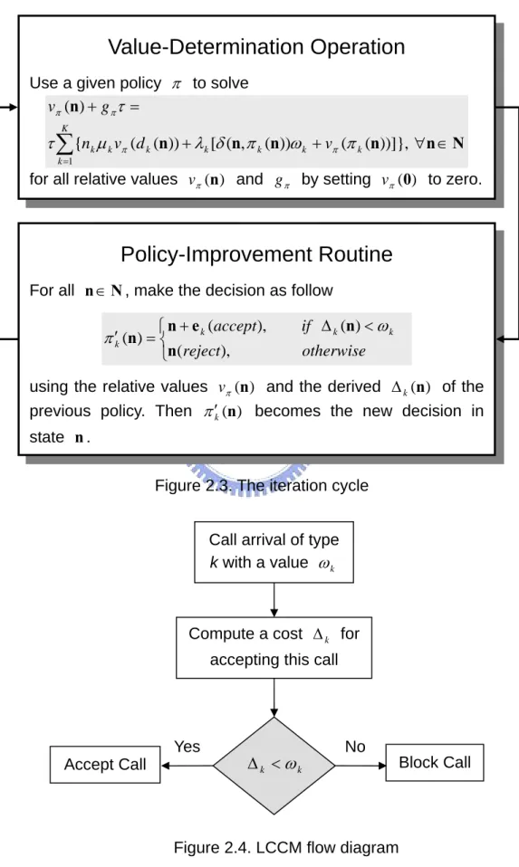
(19) Value-Determination Operation Use a given policy π to solve vπ (n) + g π τ = K. τ ∑{nk µ k vπ (d k (n)) + λk [δ (n, π k (n))ω k + vπ (π k (n))]}, ∀n ∈ N k =1. for all relative values vπ (n) and g π by setting vπ (0) to zero.. Policy-Improvement Routine For all n ∈ N , make the decision as follow. ⎧n + e k (accept ), ⎩n(reject ),. π k′ (n) = ⎨. if ∆ k (n) < ω k otherwise. using the relative values vπ (n) and the derived ∆ k (n) of the previous policy. Then π k′ (n) becomes the new decision in state n . Figure 2.3. The iteration cycle Call arrival of type k with a value ω k. Compute a cost ∆ k for accepting this call. Yes Accept Call. ∆ k < ωk. No Block Call. Figure 2.4. LCCM flow diagram. 12.

(20) and find the sub-optimal policy to solve our problem. We define the base policy π 0 which is used to determinate the relative cost and to find the next policy π 1 . We proposed this control method, called Least Cost Control in Multi-Service Networks (LCCM), shown in Figure 2.4. Lemma 2 With two policies denoted by π 0 and π 0′ , such that. g π 0 ≤ g π 0′ we have. g π1 ≤ g π1′ where π 1 and π 1′ are the next policy based on π 0 and π 0′ respectively. Proof: Recall from [1] that if we had an optimal policy during the time interval [0, t ] we could find the best alternative in [t , t + τ ] by minimizing K. ∑ λ [δ (n, π k. k =1. k. (n))ω k + Vπ (t | n 0 = π k (n))]. ∀n ∈ N. (2.18). here we find (2.18) is different from (2.14) by t = 0 . Use (2.4) to modify (2.18), we have the best alternative by minimizing K. ∑ λ [δ (n, π k =1. k. k. (n))ω k + ( g π 0 t + vπ (π k (n)))]. ∀n ∈ N. (2.19). where t is large enough. Since g π 0 ≤ g π 0′ , we obtain from [6] and have K. min ∑ λ k [δ (n, π 0 k (n))ω k + ( g π 0 t + vπ 0 (π 0 k (n)))] ≤ π 0k. k =1 K. min ∑ λ k [δ (n, π 0′ k (n))ω k + ( g π 0′ t + vπ 0′ (π 0′ k (n)))] π 0′ k. ∀n ∈ N. (2.20). k =1. where g π 0 t + vπ 0 (n) approximates to g π 0 t when t is large. The RHS. 13.

(21) (Right Hand Side) and LHS (Left Hand Side) of (2.20) are denoted by. Vπ 1 (t + τ | n 0 = π 1k (n)) and Vπ 1′ (t + τ | n 0 = π 1′k (n)) respectively. As the same policies, we rewrite equation (2.20) as K. ∑ λ [δ (n, π k =1. k. 1k. (n))ω k + ( g π 1 t ′ + vπ 1 (π 1k (n)))] ≤. K. ∑ λ [δ (n, π ′ (n))ω k =1. k. 1k. k. ∀n ∈ N, t ′ ∈ R. (2.21). + ( g π 1′ t ′ + vπ 1′ (π 1′k (n)))]. It is equivalent as Vπ 1 (t ′ | n 0 = π 1k (n)) ≤ Vπ 1′ (t ′ | n 0 = π 1′k (n)) (t ′ → ∞) or g π 1 t ′ + vπ 1 (π 1k (n)) ≤ g π 1′ t ′ + vπ 1 (π 1′k (n)). (t ′ → ∞). (2.22). then we have g π1 ≤ g π1′ by approximation. . 2.4 The Guard Channel Policy in SingleService Network We have an important result from Lemma 1 that an initial policy is considerable. We show that the notion of guard channels was introduced in the mid-80s [9,10]. It is a good choice to be our initial policy because of simplicity and optimization. We compute performance of the admission policies based on the following assumptions: The arrival process of new and handoff calls is Poisson with λn and λh . Let λ = λ n + λ h and λ h = αλ .. 14.

(22) The channel holding time for both type of calls is exponentially distributed with mean 1 µ and let ρ = λ µ . The busy-line effect is negligible, i.e., the interval between two calls from a MS is much greater than the mean call holding time. Define the state of a cell at time t by the total number of occupied channels. Thus, the cell channel occupancy can be modeled by a continuous time Markov chain with C states. The state transition rate diagram of a cell with C channels and C − T guard channels is shown in Figure 2.5. Lemma 3 In single-service network, the guard channel policy is the optimal admission control policy that minimizes a linear objective function of the new and handoff call blocking probabilities as. F = min(λ n ⋅ Bn ⋅ ω n + λ h ⋅ Bh ⋅ ω h ). (2.23). for a given C, and given constants ω n and ω h with 0 < ω n < ω h . Proof: Given in [2].. λ 0. λ. 2µ. Tµ. αλ. αλ T+1. T. 1. µ. λ. (T + 1) µ. C-1. (C − 1) µ. C Cµ. Figure 2.5. State transition diagram (Guard Channel Scheme) In next chapter, we compute the relative cost used two kinds of policies in detail and make comparison with each other.. 15.

(23) Chapter 3 Evaluation for the Relative Cost in Detail In this chapter, we use two kinds of policies to compute the relative cost values vπ (n) for all n ∈ N .. 3.1 The Dedicated Bandwidth Policy ( π 0 ) Now we assume that each call type has a portion of link bandwidth C k dedicated to it such that K. C = ∑ Ck. (3.1). k =1. In other words, the bandwidth is divided into K pieces. Let us now define the policy π 0 . Definition 1 The policy π 0 is defined by the requirement that when the state of the channel is n ∈ N an incoming call of type k (k = 1,L , K ) is accepted if and only if. C k − nk a k ≥ a k. (3.2). where nk is the number of calls of type k, currently in progress: otherwise, the call is rejected and the state of the link left unchanged.. Remark 1. 16.

(24) Although the states of the link which are recurrent under π 0 are precisely those in which nk a k ≤ C k , (k = 1,L, K ) , the policy π 0 is nevertheless defined for all n ∈ N , and so can be used as a starting point for the policy improvement routine. From Remark 1 it is clear that we have to compute relative cost values for all states, not only for those which are recurrent under the policy π 0 . We underline that the next policy, π 1 , is derived from the relative cost values of all states. Based on this, we introduce the following definition: Definition 2 We say that service k “borrows” capacity if the bandwidth used by this service is greater than the corresponding dedicated bandwidth; in other words: nk a k > C k . Strictly speaking, borrowing capacity under π 0 can happen only if at the initial state some service uses more bandwidth than its allocated portion. After some finite transient period, all services will be using only bandwidth allocated to them. On the contrary, the next policy allows calls of one service to take a portion of bandwidth allocated to another service if the cost for that is less than a given call reward. We assume that there are two types of service, narrowband (NB) and wideband (WB). Each type of service has also two type of arrival, new call and handoff call, hence our traffic is divided into four classes of service ( K = 4) , each class corresponding to a different type of traffic. Type 1 and type 2 represent the new call and handoff call of NB respectively. In the same way, type 3 and type 4 represent the new call and handoff call of WB respectively. We make the following assumptions: Call arrive according to a stationary Poisson process with mean rate λk . Call holding times are independent and have a negative exponential distribution with mean 1 µ k , and with the property of memoryless we. 17.

(25) have ⎧ µ12 = µ1 = µ 2 , ⎨ ⎩µ 34 = µ 3 = µ 4. Each blocked call incurs immediate cost denoted by ω k . Definition 3. n ( k ) is the vector n with the component k set to zero. Lemma 4 If k does not borrow resources from j at t = 0 , then taking either. n or n ( k ) as an initial system state at t = 0 , we will obtain the same driving process n j (t ) . Proof: It is obvious from the definition of π 0 . Lemma 5 If k does not borrow resources from j at t = 0 , then. vπ( 0j ) (n) = vπ( 0j ) (n ( k ) ). (3.3). Proof: Given in [3]. In the four-service case ( K = 4) under the policy π 0 , the channel state space Ν is divided into four region, namely N I , N II , N III , and N VI , are defined as follows:. N = N I I N II I N III I N VI N I = {n : n1 a1 ≤ C1 ∩ n 2 a 2 ≤ C 2 ∩ n3 a3 ≤ C 3 ∩ n 4 a 4 ≤ C 4 } N II = {n : [n1 a1 > C1 ∩ n2 a 2 ≤ C 2 ∩ n3 a3 ≤ C 3 ∩ n4 a 4 ≤ C 4 ] ∪. 18.

(26) [n1 a1 ≤ C1 ∩ n2 a 2 > C 2 ∩ n3 a3 ≤ C 3 ∩ n 4 a 4 ≤ C 4 ] ∪ [n1 a1 ≤ C1 ∩ n2 a 2 ≤ C 2 ∩ n3 a3 > C 3 ∩ n4 a 4 ≤ C 4 ] ∪ N III. [n1 a1 ≤ C1 ∩ n2 a 2 ≤ C 2 ∩ n3 a3 ≤ C 3 ∩ n4 a 4 > C 4 ]} = {n : [n1 a1 > C1 ∩ n 2 a 2 > C 2 ∩ n3 a3 ≤ C 3 ∩ n 4 a 4 ≤ C 4 ] ∪ [n1a1 ≤ C1 ∩ n2 a 2 ≤ C 2 ∩ n3 a3 > C3 ∩ n4 a 4 ≤ C 4 ] ∪ [n1a1 ≤ C1 ∩ n2 a 2 ≤ C 2 ∩ n3 a3 ≤ C3 ∩ n4 a 4 > C 4 ] ∪ [n1a1 ≤ C1 ∩ n2 a 2 > C 2 ∩ n3 a3 > C3 ∩ n4 a 4 ≤ C 4 ] ∪. (3.4). [n1a1 ≤ C1 ∩ n2 a 2 > C 2 ∩ n3 a3 ≤ C3 ∩ n4 a 4 > C 4 ] ∪ N VI. [n1a1 ≤ C1 ∩ n2 a 2 ≤ C 2 ∩ n3 a3 > C3 ∩ n4 a 4 > C 4 ]} = {n : [n1 a1 > C1 ∩ n 2 a 2 > C 2 ∩ n3 a3 > C 3 ∩ n4 a 4 ≤ C 4 ] ∪ [n1 a1 > C1 ∩ n 2 a 2 > C 2 ∩ n3 a3 ≤ C 3 ∩ n 4 a 4 > C 4 ] ∪ [n1 a1 > C1 ∩ n 2 a 2 ≤ C 2 ∩ n3 a3 > C 3 ∩ n4 a 4 > C 4 ] ∪ [n1 a1 ≤ C1 ∩ n2 a 2 > C 2 ∩ n3 a3 > C 3 ∩ n4 a 4 > C 4 ]}. These region are helpful to reduces the four-dimensional problem to more tractable one-dimensional problem. It is important to emphasize that we did not use any approximations.. 3.1.1 Cost function in region Ⅰ From (3.4), it follows that there is no borrowing of capacity in N I . In the following figure, we depict the state transitions in the one-dimensional Markov chain.. λk. λk Nk −1. ( N k − 1) µ k. N k = Ck ak Nk +1. Nk. ( N k + 1) µ k. N k µk. Figure. 3.1 State transitions in regionⅠ. 19.

(27) Note that in Figure. 3.1 we also consider the states outside the dedicated region, in which, according to π 0 , there are no call arrivals. Since there is no borrowing of capacity, we are interested in finding the denoted by θ (nk ) . We also define. difference vπ(k0 ) (n k + 1) − vπ( k0 ) (nk ). ρ k = λk µ k , N k = ⎣C k a k ⎦ , and M k = ⎣C a k ⎦ . Then we can find the solution of θ (nk ) as θ (nk ) =. E(N k , ρk ) , E (nk , ρ k ). n k ∈ [1, N k − 1]. (3.5a). θ (nk ) =. E( N k , ρk ) , E (nk , ρ k ). nk > N k. (3.5b). gπ( k0 ) = λk E ( N k , ρ k ).. (3.5c). The proof is given in [4] and the Erlang-B formula is. E(N , ρ ) =. ρ N N! N. ∑ρ. i. .. (3.6). i!. i =0. Now, the cost of accepting is simply. ∆ k = θ (nk )ω k .. (3.7). and the relative cost value function is found as vπ 0 ( n k ) = (k ). nk −1. ∑θ (i) .. (3.8). i =0. In conclusion, the cost of routing a type-k call with the current state in N I is obtained by (3.5a) and (3.7), and can be computed in real-time applications as well (3.5b) will be used in other regions.. 20.

(28) 3.1.2 Cost function in region Ⅱ Next, we consider the subspace N II where there is a service borrows resources from another service. Let us first find the cost of accepting a type 1 call. In this case, we assume that type 2 borrows resource from type 1. Given N 2 = ⎣C 2 a 2 ⎦ , N 3 = ⎣C 3 a3 ⎦ and N 4 = ⎣C 4 a 4 ⎦ , let the current channel state is n = (n1 , n2 , n3 , n4 ) ∈ N II where n 2 = N 2 + 1 , 0 ≤ n3 ≤ N 3 and 0 ≤ n 4 ≤ N 4 . Then, the task is to find the relative cost vπ(10) (n1 , n2 , n3 , n4 ) where ω1 = 1 , ω 2 = 0 , ω 3 = 0 , and ω 4 = 0 . The state transition diagram in the second region is shown in Figure. 3.2. The idea is not to solve the whole system of linear equations, but the system relevant for region Ⅱ . It is already shown in (3.8) that,. n1 , N 2 + 2 ( N 2 + 2) µ 2. λ1. λ1 n1 , N 2 + 1. n1 − 1, N 2 + 1 n1 µ1. n1 + 1, N 2 + 1. (n1 + 1) µ1 ( N 2 + 1) µ 2 n1 , N 2. Figure. 3.2 State transitions in region Ⅱ. 21.

(29) regardless of n 2 (0 ≤ n 2 ≤ N 2 ) , vπ(10) (n1 , n2 , n3 , n4 ) =. where. θ (⋅). is. given. by. nk −1. ∑θ (i),. ∀(n1 , n 2 , n3 , n 4 ) ∈ N I .. (3.5a).. Therefore,. i =0. all. (3.9). relative. vπ(10) (n1 , N 2 , n3 , n 4 ) on the boundary between N I and N II. values. (0 ≤ n1 ≤ N 1 ,. 0 ≤ n3 ≤ N 3 ,0 ≤ n4 ≤ N 4 ) are known. In order to find the relative cost values for all possible states, we denote the resource of type-k borrowed from type-j by b jk (n) FCUs for all n ∈ N . We will compute all b jk (n) for all n ∈ N later. Next, we form the system of linear equations for the states on the line above region Ⅰ, defined by M 1 = ⎣(C1 − b12 (n)) a1 ⎦ , N 1 = ⎣(C − n2 a 2 − n3 a3 − n4 a 4 ) a1 ⎦ , n 2 = N 2 + 1 , 0 ≤ n3 ≤ N 3 and 0 ≤ n 4 ≤ N 4 . This system can be put in the following matrix form: A II v II = f II ,. (3.10). where ⎡ a 0 c0 0 0 L ⎢b a c1 0 L 1 ⎢ 1 ⎢ 0 b2 a 2 c 2 L ⎢ ⎢L L L L L ⎢0 0 0 0 L A II = ⎢ ⎢0 0 0 0 L ⎢0 0 0 0 L ⎢ ⎢L L L L L ⎢0 0 0 0 L ⎢ ⎢⎣ 0 0 0 0 L ⎡ vπ 0 ( 0 , n2 , n3 , n4 ) ⎤ ⎥ ⎢ (1 ) ⎢ vπ 0 (1, n2 , n3 , n4 ) ⎥ ⎥ ⎢ L v II = ⎢ (1) ⎥ , ⎢ vπ 0 ( M 1 , n2 , n3 , n4 ) ⎥ ⎥ ⎢ L ⎥ ⎢ (1 ) ⎢⎣ vπ 0 ( N 1 , n2 , n3 , n4 ) ⎥⎦ (1 ). 0. 0. 0. L. 0. 0. 0 0. 0 0. 0 0. L L. 0 0. 0 0. L a M 1 −1. L c M 1 −1. L 0. L L. L 0. L 0. bM 1 0. aM 1 bM 1 + 1. 0 a M 1 +1. L L. 0 0. 0 0. L 0. L 0. L 0. L L. L b N 1 −1. L a N 1 −1. 0. 0. 0. L. 0. bN 1. ⎡ f0 ⎤ ⎢f ⎥ ⎢ 1 ⎥ ⎢L ⎥ ⎥ f II = ⎢ ⎢ fM1 ⎥ ⎢L ⎥ ⎥ ⎢ ⎢⎣ f N 1 ⎥⎦. 22. 0 ⎤ 0 ⎥⎥ 0 ⎥ ⎥ L⎥ 0 ⎥ ⎥ , 0 ⎥ 0 ⎥ ⎥ L⎥ 0 ⎥ ⎥ a N 1 ⎥⎦. (3.11).

(30) The coefficients in A II and f II are given as. ai = 1,. i ∈ [0, N 1 ]. λ1 , iµ1 + n 2 µ 2 + λ1 iµ 1 , bi = − iµ1 + n 2 µ 2 + λ1 iµ 1 , bi = − iµ 1 + n 2 µ 2 ci = −. fi = fi =. i ∈ [0, M 1 − 1] i ∈ [1, M 1 − 1] i ∈ [M 1 , N1 ]. n2 µ 2 vπ(10) (i, n2 − 1, n3 , n4 ) − g π(10) iµ1 + n2 µ 2 + λ1. n2 µ 2 vπ(10) (i, n2 − 1, n3 , n4 ) − g π(10) + λ1 iµ 1 + n 2 µ 2. i ∈ [0, M 1 − 1]. ,. (3.12). ,. i ∈ [M 1 , N1 ]. We can find the solution of (3.10) by. v II = A -1II f II ,. (3.13). Thus, given the channel state (n1 , N 2 + 1, n3 , n4 ) , the cost of accepting a type-1 call is simply ∆ 1 = [vπ(10) (n1 + 1, N 2 + 1, n3 , n 4 ) − vπ(10) (n1 , N 2 + 1, n3 , n 4 )]ω1. (3.14). where the relative cost values are computed by (3.13). We can also find the cost in channel state (n1 , n2 , N 3 + 1, n4 ) and (n1 , n2 , n3 , N 4 + 1) in the same approach. This way gives us an idea of how to find the relative value for any state in the second region. We divide the subspace N II into lines representing states with the same number of type-2 calls. First, we compute the relative values for n 2 = N 2 + 1 . Then, in the next iteration, we find the relative values n 2 = N 2 + 2 , and so on. The process is stopped when the relative. 23.

(31) values for all states in N II are determined. This iterative procedure is more efficient with respect to computation time and memory space than any other method which solves the system of linear equations for the whole space N .. 3.1.3 Cost function in region Ⅲ We continuously consider the subspace N III that the second service and the third borrow form the first service for example. In other wards, there are two kinds of service exceeding their dedicated bandwidth. In this. n1 , N 2 + 2. n1 , N 2 + 1. N3 + 1. N3 + 2. ( N 2 + 2) µ 2. ( N 3 + 2) µ 3. λ1. λ1. n1 − 1, N 2 + 1,. n1 , N 2 + 1,. n1 + 1, N 2 + 1. N3 + 1. N3 + 1. N3 + 1 (n1 + 1) µ1. n1 µ1. ( N 3 + 1) µ 3. ( N 2 + 1) µ 2. n1 , N 2 + 1,. n1 , N 2 ,. N3. N3 + 1. Figure. 3.3 State transitions in region Ⅲ case, we neglect the influence of type-4 by Lemma 4. Given N 2 = ⎣C 2 a 2 ⎦ , N 3 = ⎣C 3 a3 ⎦ and N 4 = ⎣C 4 a 4 ⎦ , let the current channel state is. 24.

(32) n = (n1 , n2 , n3 , n4 ) ∈ N III where n 2 = N 2 + 1 , n3 = N 3 + 1 and 0 ≤ n4 ≤ N4 . Next, We want to find the relative cost values vπ(10) (n1 , n 2 , n3 , n 4 ) where. ω1 = 1 , ω 2 = 0 , ω 3 = 0 , and ω 4 = 0 . The state transition diagram in the third region is shown in Figure. 3.3. Given M1 = ⎣(C1 − b12 (n) − b13 (n)) / a1 ⎦ , N1 = ⎣(C − n2 a2 − n3 a3 − n4 a4 ) a1 ⎦ , n 2 = N 2 + 1 , n3 = N 3 + 1 and 0 ≤ n 4 ≤ N 4 ,. we have A III v III = f III ,. (3.15). where. A III. v III. ⎡a 0 ⎢b ⎢ 1 ⎢0 ⎢ ⎢L ⎢0 =⎢ ⎢0 ⎢0 ⎢ ⎢L ⎢0 ⎢ ⎢⎣ 0. c0. 0. 0. L. 0. 0. 0. L. 0. 0. a1 b2. c1 a2. 0 c2. L L. 0 0. 0 0. 0 0. L L. 0 0. 0 0. L c M 1 −1. L 0. L L. L 0. L 0. 0. L. 0. 0. a M 1 +1 L L L. 0 L. 0 L. L L L L L 0 0 0 L a M 1 −1 L. bM 1. a M1. 0 0 0 L L L L L. 0 L. bM 1 +1 L. L L. 0 0. 0 0. 0. 0 0. 0. 0 0. 0. 0 0. 0 0. L b N1 −1 L 0. a N1 −1 b N1. 0 ⎤ 0 ⎥⎥ 0 ⎥ ⎥ L⎥ 0 ⎥ ⎥ , 0 ⎥ 0 ⎥ ⎥ L⎥ 0 ⎥ ⎥ a N1 ⎥⎦. ⎡ f0 ⎤ ⎡ vπ(10) (0, n 2 , n3 , n 4 ) ⎤ ⎢f ⎥ ⎥ ⎢ (1) ⎢ 1 ⎥ ⎢ vπ 0 (1, n 2 , n3 , n 4 ) ⎥ ⎢L ⎥ ⎥ ⎢ L ⎥ = ⎢ (1) ⎥ , f III = ⎢ ⎢ f M1 ⎥ ⎢ vπ 0 ( M 1 , n 2 , n 3 , n 4 ) ⎥ ⎢L ⎥ ⎥ ⎢ L ⎥ ⎢ ⎥ ⎢ (1) ⎢⎣ f N1 ⎥⎦ ⎢⎣ vπ 0 ( N 1 , n 2 , n3 , n 4 ) ⎥⎦. (3.16) The coefficients in A III and f III are given as. 25.

(33) ai = 1, ci = − bi = − bi = − fi = fi =. i ∈ [0, N 1 ]. λ1. ,. i ∈ [0, M 1 − 1]. iµ1 , iµ1 + n2 µ 2 + n3 µ 3 + λ1. i ∈ [1, M 1 − 1]. iµ1 + n2 µ 2 + n3 µ 3 + λ1. iµ 1 iµ 1 + n 2 µ 2 + n 3 µ 3. i ∈ [ M 1 , N1 ]. ,. n2 µ 2 vπ(10) (i, n2 − 1, n3 , n4 ) − g π(10) iµ1 + n2 µ 2 + n3 µ 3 + λ1. i ∈ [0, M 1 − 1]. ,. n2 µ 2 vπ(10) (i, n2 − 1, n3 , n4 ) + n3 µ 3 vπ(10) (i, n2 , n3 − 1, n4 ) − g π(10) + λ1 iµ 1 + n 2 µ 2 + n 3 µ 3. ,. i ∈ [M 1 , N1 ] (3.17). We can find the solution of (3.15) by. v III = A -1III f III ,. (3.18). Thus, given the channel state (n1 , N 2 + 1, N 3 + 1, n4 ) , the cost of accepting a type-1 call is simply ∆ 1 = [vπ(10) (n1 + 1, N 2 + 1, N 3 + 1, n 4 ) − vπ(10) (n1 , N 2 + 1, N 3 + 1, n 4 )]ω1. (3.19). where the relative cost values are computed by (3.18). We can also find the cost in channel state (n1 , N 2 + 1, n3 , N 4 + 1) and (n1 , n2 , N 3 + 1, N 4 + 1) in the same approach. So does ∆ 2 , ∆ 3 , and ∆ 4 in region Ⅲ.. 3.1.4 Cost function in region Ⅳ Finally, we compute the relative cost values when there are three types of service exceeding their dedicated bandwidth respectively. Given N 2 = ⎣C 2 a 2 ⎦ , N 3 = ⎣C 3 a3 ⎦ and N 4 = ⎣C 4 a 4 ⎦ , we are going to find the. 26.

(34) n1 , N 2 + 1 N 3 + 1, N 4 + 2 n1 , N 2 + 2. n1 , N 2 + 1. N 3 + 1, N 4 + 1. N 3 + 2, N 4 + 1. ( N 4 + 2) µ 4 ( N 2 + 2) µ 2. ( N 3 + 2) µ 3. λ1. λ1 n1 , N 2 + 1,. n1 − 1, N 2 + 1,. n1 + 1, N 2 + 1. N 3 + 1, N 4 + 1. N 3 + 1, N 4 + 1. N 3 + 1, N 4 + 1. (n1 + 1) µ1. n1 µ1. ( N 3 + 1) µ 3. ( N 2 + 1) µ 2. ( N 4 + 1) µ 4 n1 , N 2 + 1, N3 , N4 + 1. n1 , N 2 , N 3 + 1, N 4 + 1. n1 , N 2 + 1 N 3 + 1, N 4. Figure. 3.4 State transitions in region Ⅳ cost vπ(10) (n1 , n 2 , n3 , n 4 ) where n 2 = N 2 + 1 , n3 = N 3 + 1 and n 4 = N 4 + 1 . The state transition diagram in the fourth region is shown in Figure. 3.4. Given M1 = ⎣(C − n2a2 − n3a3 − n4a4 ) a1 ⎦ , n2 = N2 + 1 , n3 = N3 +1 and n4 = N4 +1 ,. we have. A IV v VI = f IV , where. 27. (3.20).

(35) A IV. v IV. ⎡a 0 ⎢b ⎢ 1 ⎢0 =⎢ ⎢L ⎢0 ⎢ ⎢⎣ 0. c0. 0. L. 0. 0. a1. c1. L. 0. 0. b2 a 2 L L L L. 0 L. 0 L. 0 0. 0 0. L bM 1 −1 0 L. a M 1 −1 bM 1 −. 0 ⎤ 0 ⎥⎥ 0 ⎥ ⎥ , L ⎥ c M 1 −1 ⎥ ⎥ a M 1 ⎥⎦. (3.21). ⎡ vπ(10) (0, n 2 , n3 , n 4 ) ⎤ ⎡ f0 ⎤ ⎥ ⎢ (1) ⎢f ⎥ vπ 0 (1, n 2 , n3 , n 4 ) ⎥ 1 ⎥ ⎢ , f IV = ⎢ = ⎥ ⎢ ⎢ L ⎥ L ⎥ ⎢ (1) ⎥ ⎢ ⎢⎣vπ 0 ( M 1 , n 2 , n3 , n 4 ) ⎥⎦ ⎣⎢ f M 1 ⎦⎥. The coefficients in A IV and f IV are given as. ai = 1,. i ∈[0, N1 ]. λ1 , iµ1 + n2 µ2 + n3µ3 + n4 µ4 + λ1 iµ1 bi = − , iµ1 + n2 µ2 + n3µ3 + n4 µ4 + λ1 iµ1 bi = − , iµ1 + n2 µ2 + n3µ3 + n4 µ4 ci = −. i ∈[0, M1 −1] i ∈[1, M1 −1] i = M1. fi = [n2 µ2vπ(10) (i, n2 −1, n3 , n4 ) + n3µ3vπ(10) (i, n2 , n3 −1, n4 ) +. i ∈[0, M1 −1]. n4 µ4vπ(10) (i, n2 , n3 , n4 −1) − gπ(10) + λ1 ] /(iµ1 + n2 µ2 + n3µ3 + n4 µ4 + λ1 ), fi = [n2 µ2vπ(10) (i, n2 −1, n3 , n4 ) + n3µ3vπ(10) (i, n2 , n3 −1, n4 ) + n4 µ4vπ(10) (i, n2 , n3 , n4 −1) − gπ(10) + λ1 ] /(n2 µ2 + n3µ3 + n4 µ4 + λ1 ),. i = M1 (3.22). We can find the solution of (3.20) by. v IV = A -1IV f IV ,. 28. (3.23).

(36) Here is the end for calculations of all relative cost values for all n ∈ N . Using the Lemma in [3], the channel cost of accepting a type-k call is given as 4. ∆ k = ∑ [vπ( 0j ) (n + e j ) − vπ( 0j ) (n)]ω j. (3.24). j =1. 3.1.5 Service bandwidth allocation We assume that each call class has a portion of channel bandwidth, denoted by C k , which is dedicated to it such that. C k − nk a k ≥ a k. (3.25). Also, we recall that the objective is to minimize the equilibrium excepted cost per unit time that is given as 4. g π 0 = ∑ g π( k0 )ω k. (3.26). k =1. where gπ( k0 ) is obtained by (3.5c). From (3.25) and (3.26), it is obvious that the appropriate choice of N k ’s is the solution of the following optimization problem: 4. min. N1 , N 2 , N 3 , N 4. ∑λ k =1. k. E ( N k , ρ k )ω k. (3.27). subject to. N 1 a1 + N 2 a 2 + N 3 a3 + N 4 a 4 ≤ C .. (3.28). Knowing the N k ’s, we are able to find the dedicated bandwidth for each. 29.

(37) type of service as C k = N k a k . Since E ( N , ρ ) is a convex and monotonically decreasing function with respect to channel capacity N when ρ is constant, the solution lies at the line N 1 a1 + N 2 a 2 + N 3 a3 + N 4 a 4 = C . Thus, the minimum of (3.27) can be found by the exhaustive search method.. 3.2 The Guard Channel Policy ( π 0′ ) In order to find the better policy in next step, we use the Guard Channel policy as the initial policy since its gain is smaller than the divided one. Also, the Guard Channel policy provide more simple and efficient calculation by reducing the dimension of Markov chain. Fortunately, we can follow the same flow in section 3.1 to find the relative cost values for all n∈N. In wireless network, each call type of service can be distinguished into “new” and “handoff” call. We denote the type-1 call and the type-2 call as the new call and the handoff call of the narrow band service respectively. Similarly, the type-3 call and the type-4 call are denoted as the new call and the handoff call of the wideband service respectively. We define the dedicated bandwidth C12 and C 34 as. C = C12 + C 34. (3.29). where C is the total bandwidth. Continuously, let us denoted by T12 and T34 the threshold reserved a subset of these channels (say C12 − T12 and C 34 − T34 ) for handoff call, type-2 and type-4 call. Also, the capacity requirement of each call denoted by a k , we define as follow ⎧ a 12 ⎪ ⎪ ⎨ ⎪ a 34 ⎪⎩. = a1 = a2 , = a3 = a4. 30. (3.30).

(38) Then the policy π 0′ is defined as follows: Definition 4 The policy π 0′ is defined by the requirement that when the state of the channel is n ∈ N an incoming call of type k (k = 1, L,4) is accepted if and only if ⎧n1 + n2 < T12 , ⎪C − (n + n )a ≥ a , ⎪ 12 1 2 12 12 ⎨ + < , n n T 4 34 ⎪ 3 ⎪⎩C 34 − (n3 + n 4 )a34 ≥ a34 ,. k =1 k =2 k =3. (3.31). k =4. where nk is the number of calls of type k (k = 1, L,4) , currently in progress: otherwise, the call is rejected and the state of the link left unchanged. Here we have the following lemma: Lemma 6 For the Guard Channel policy π 0′ , the relative value function vπ 0′ (n1 , n 2 , n3 , n 4 ) can be expressed as. ⎧⎪vπ(10′) (n1 , n2 , n3 , n4 ) + vπ( 20′ ) (n1 , n2 , n3 , n4 ) = vπ(120′ ) (n1 + n 2 , n3 + n4 ) ⎨ ( 3) ( 4) ( 34 ) ⎪⎩vπ 0′ (n1 , n 2 , n3 , n 4 ) + vπ 0′ (n1 , n 2 , n3 , n4 ) = vπ 0′ (n1 + n 2 , n3 + n4 ). (3.32). where vπ(120′ ) (n1 + n 2 , n3 + n4 ) is the solution of the system (2.9) in the case. ω 3 = 0 and ω 4 = 0 , and vπ(12′ ) (n1 + n2 , n3 + n4 ) is the solution of the system 0. (2.9) in the case ω1 = 0 and ω 2 = 0 . Proof: It is obvious from the definition of π 0′ and Lemma 1.. 31.

(39) In the four-service case ( K = 4) under the policy π 0′ , the channel state space Ν is divided into three region, namely N I , N II , and N III , are defined as follows:. N = N I I N II I N III N I = {n : n1 a1 + n2 a 2 ≤ C12 ∩ n3 a3 + n4 a 4 ≤ C 34 }. (3.33). N II = {n : n3 a3 + n4 a 4 > C 34 } N III = {n : n1 a1 + n2 a 2 > C12 }. 3.2.1 Cost function in region Ⅰ. C12. From (3.33), it follows that there is no borrowing of capacity (within or C 34 ) in N I . Here we take an example for computation of the. relative cost value vπ(120′ ) (n1 + n2 , n3 + n4 ) . Given N12 = ⎣C12 /a12⎦ and M12 = ⎣C / a12 ⎦ the state transition diagram for type-1 and type-2 calls in the first region is shown in Figure. 3.5.. λ1 + λ 2. λ1 + λ 2 T12 T12 µ12. T12. (T12 + 1)µ12. λ2. λ2 N 12 − 1. ( N 12 − 1) µ12 N12 µ12. N 12. N 12 + 1. ( N 12 + 1) µ12. Figure. 3.5 State transitions in regionⅠfor type-1 and type-2 calls Denoted by n3 + n4 ≤ ⎣C 34 / a34 ⎦ , next we form the system of linear equations for the state in region Ⅰ as: A ′I v ′I = f I′,. where. 32. (3.34).

(40) ⎡a 0 c 0 0 ⎢b a c 1 1 ⎢ 1 ⎢L L L ⎢ ⎢0 0 0 ⎢0 0 0 ⎢ A ′I = ⎢ 0 0 0 ⎢0 0 0 ⎢ ⎢0 0 0 ⎢0 0 0 ⎢ ⎢0 0 0 ⎢ ⎣0 0 0. L. 0. 0. 0. 0. 0. 0. 0. L. 0. L L. 0 L. 0 L. 0 L. 0 L. 0 L. 0 L. 0 L L L. 0 L. cT12 −1 aT12 0. 0 cT12 0. 0 0 L. 0 0 0. 0 0 0. 0 0 0. L L L. 0 0 0 0 0. L aT12 −1 L bT12 0 L L L. 0 0. 0 0. 0 0. 0 0. a M 12 −1 bM 12. c M 12 −1 a M 12. 0 0. L L. L L. 0 0. 0 0. 0 0. 0 0. 0 0. 0 0. 0 0. 0 L L a N12 −1. L. 0. 0. 0. 0. 0. 0. 0. L. ⎡ vπ(120′ ) (0, n3 + n 4 ) ⎤ ⎢ ⎥ (12 ) ⎢ vπ 0′ (1, n3 + n 4 ) ⎥ ⎢ ⎥ L ⎢v (12 ) (T − 1, n + n )⎥ 3 4 ⎢ π 0′ 12 ⎥ (12 ) ⎢ ′ v I = vπ 0′ (T12 , n3 + n 4 ) ⎥ ⎢ ⎥ L ⎢ (12 ) ⎥ ⎢ vπ 0′ ( M 12 , n3 + n 4 ) ⎥ ⎢ ⎥ L ⎢ ⎥ ⎢ vπ(12′ ) ( N 12 , n3 + n 4 ) ⎥ ⎣ 0 ⎦. ⎡ f0 ⎤ ⎢ ⎥ ⎢ f1 ⎥ ⎢ L ⎥ ⎢ ⎥ ⎢ f T12 −1 ⎥ ⎢ ⎥ f I′ = ⎢ f T12 ⎥ ⎢ L ⎥ ⎢ ⎥ ⎢ f M 12 ⎥ ⎢ ⎥ ⎢ L ⎥ ⎢ fN ⎥ ⎣ 12 ⎦. b N12. 0 ⎤ 0 ⎥⎥ L⎥ ⎥ 0 ⎥ 0 ⎥ ⎥ 0 ⎥ 0 ⎥ ⎥ 0 ⎥ 0 ⎥ ⎥ 0 ⎥ ⎥ a N12 ⎦. (3.35). The coefficients in A ′I and f I′ are given as. ai′ = 1,. i ∈ [0, N 12 ]. λ1 + λ 2 , iµ12 + λ1 + λ 2 λ2 ci′ = − , iµ12 + λ 2 iµ12 bi′ = − , iµ1 2 + λ1 + λ 2 iµ12 bi′ = − , iµ12 + λ 2 ci′ = −. i ∈ [0, T12 − 1] i ∈ [T12 , M 12 − 1] (3.36). i ∈ [1, T12 − 1] i ∈ [T12 , M 12 − 1]. bi′ = −1,. i ∈ [ M 12 , N 12 ]. 33.

(41) f i′ =. λ 1ω 1 − g π(12′ ) , iµ 1 + λ 2. f i′ =. λ 1ω 1 + λ 2 ω 2 − g iµ 1. i ∈ [T12 , M 12 − 1]. 0. ( 12 ) π 0′. (3.37). i ∈ [ M 12 , N 12 ]. ,. We can find the solution of (3.34) by. v ′I = ( A ′I ) -1 f I′,. (3.38). 3.2.2 Cost function in region Ⅱ In this section, we consider the subspace N II where the second service (type-3 and type-4) borrows resources from the first service. Given M 12 = ⎣C − (n3 + n4 )a34 / a12 ⎦ , N 34 = ⎣C 34 / a34 ⎦ 0 ≤ n1 + n 2 ≤ M 12 , and n3 + n4 = N 34 + 1 , the system also can put in the following matrix form: A ′II v ′II = f II′ ,. (3.39). where ⎡a 0 c 0 0 ⎢b a c 1 1 ⎢ 1 ⎢L L L ⎢ 0 0 0 A ′II = ⎢ ⎢0 0 0 ⎢ ⎢0 0 0 ⎢0 0 0 ⎢ ⎢⎣ 0 0 0. L L. 0 0. 0 0. 0 0. L L. 0 0. L. L. L. L. L 0. 0 L 0 L L a M 12 −1. L a T12 −1. c T12 −1. L 0. L L L. bT12 0. a T12 0. c T12 0. 0 0. 0 0. 0 0. L. L. L. b M 12. ⎡ f ⎤ ⎢ 0 ⎥ ⎢ f1 ⎥ ⎢ ⎥ ⎢ L ⎥ f II′ = ⎢ f T12 −1 ⎥ ⎢ ⎥ ⎢ f T12 ⎥ ⎢ ⎥ ⎢ L ⎥ ⎢ fM ⎥ ⎣ 12 ⎦. ⎡ v π(120′ ) (0, n 3 + n 4 ) ⎤ ⎢ ⎥ (12 ) ⎢ v π 0′ (1, n 3 + n 4 ) ⎥ ⎢ ⎥ L ⎢v (12 ) (T − 1, n + n ) ⎥ 12 3 4 v ′II = ⎢ π 0′ ⎥ ( 12 ) ⎢ v π ′ (T12 , n 3 + n 4 ) ⎥ 0 ⎢ ⎥ L ⎢ ⎥ ⎢ v π(12′ ) ( M 12 , n 3 + n 4 ) ⎥ ⎣ 0 ⎦. 34. 0 ⎤ 0 ⎥⎥ L ⎥ ⎥ 0 ⎥ 0 ⎥ ⎥ 0 ⎥ c M 12 −1 ⎥ ⎥ a M 12 ⎥⎦. (3.40).

(42) The coefficients in A ′II and f II′ are given as a i′ = 1,. i ∈ [ 0, M 12 ]. λ1 + λ 2 , iµ 12 + λ1 + λ 2 λ2 c i′ = − , iµ 12 + λ 2 iµ 12 bi′ = − , i µ 1 2 + λ1 + λ 2 iµ 12 bi′ = − , iµ 12 + λ 2 c i′ = −. f i′ = f i′ = f i′ =. i ∈ [ 0, T12 − 1] i ∈ [T12 , M 12 − 1] i ∈ [1, T12 − 1] i ∈ [T12 , M 12 ]. iµ 1 v π(120′ ) (i , n 3 + n 4 − 1) − g π(120′ ) i µ 1 + λ1 + λ 2. i ∈ [ 0, T12 − 1]. ,. iµ 1 v π(120′ ) (i , n 3 + n 4 − 1) + λ1ω 1 − g π(120′ ) iµ 1 + λ 2. iµ 1 v π(120′ ) (i , n 3 + n 4 − 1) + λ1ω 1 + λ 2 ω 2 − g π(120′ ) iµ 1. i ∈ [T12 , M 12 − 1]. , ,. i = M 12. (3.41). where the value vπ(120′ ) (i, n3 + n4 − 1) is gotten by (3.38). Hence we can find the solution of (3.39) by. v ′II = ( A ′II ) -1 f II′ ,. (3.42). According the same way in section 3.2, we compute the relative values for n3 + n4 = N 34 + 1 at first. Then, in the next iteration, we find the relative values for n3 + n4 = N 34 + 2 , and so on. The process is stopped when the relative values for all states in N II are determined. In the subspace N III , where the first service (type-1 and type-2) borrows resources from the second one (type-3 and type-4), the analysis is the same as in N II , except that what has been said for the first service is now applicable for the second one, and vice versa. Therefore, we skip the details.. 35.

(43) At the end of this section, all the relative cost values for all n ∈ N have been computed. The channel cost of accepting a type-k call is given as ∆ ′k = [vπ(120′ ) (n + e k ) − vπ(120′ ) (n)] + [vπ( 340′ ) (n + e k ) − vπ( 340′ ) (n)]. (3.43). Based on policy π 0 (or π 0′ ), we can find the relative cost values for all n ∈ N and the channel cost of accepting one type of call by (3.23) (or (3.43)). We will use these results in next chapter and make a comparison.. 3.2.3 Service bandwidth allocation Also, we recall that the objective is to minimize the equilibrium excepted cost per unit time that is given as g π 0′ = g π(120′ ) + g π( 340′ ). (3.44). where g π(12′ ) and g π( 34′ ) is obtained by (3.38). Use the result in section 3.2, 0. 0. the solution lies at the line N 12 a12 + N 34 a34 = C . Thus, the minimum of (3.44) can be found by the exhaustive search method.. 36.

(44) Chapter 4 Numerical Results In this chapter, we consider an example with two traffic services which differ in the bandwidth requirement and mean call holding time. Within each type of service, there are new call and handoff call which have different costs incurred by rejection respectively. We assume that the channel has capacity of C = 48 FCU’s. For the first service, usually a narrowband one, the relevant parameters are set as follows: a1 = a 2 = a12 = 1, µ1 = µ 2 = µ12 = 1, λ1 = 15, ω1 = 1, λ 2 = 6, ω 2 = 1.2 (4.1). Since the second service is a wideband one (a34 > a12 ) , we may assume that its mean call holding time is no less than the mean call holding time of the first service µ 34 < µ12 . In the example, we use the following parameters:. a3 = a 4 = a34 = 3, µ 3 = µ 4 = µ 34 = 0.5, λ3 = 3, ω 3 = 7, λ 4 = 1, ω 4 = 8 (4.2) In order to find the dedicated bandwidth for each class of service with the policy π 0 , we obtain from section 3.1.5 as. C1 = 17, C 2 = 7, C 3 = 18, C 4 = 6. (4.3). From section 3.2.3, it is obtained that the dedicated bandwidth with the policy π 0′ as. C12 = 21, C 34 = 27. (4.4). A channel offered load ρ , defined as 4. ρ=. ∑a k =1. k. C. ρk (4.5). is 0.9375 what considered as a heavy traffic regime. Here, ρ k = λ k µ k .. 37.

(45) n1. n2. Figure. 4.1 Channel cost ∆ 1 (⋅,⋅, n3 = 0, n4 = 0). n3. n1. Figure. 4.2 Channel cost ∆ 1 (⋅, n 2 = 0,⋅, n 4 = 0). 38.

(46) n1. n2. Figure. 4.3 Channel cost ∆ 2 (⋅,⋅, n3 = 0, n4 = 0). n3. n2. Figure. 4.4 Channel cost ∆ 2 (n1 = 0,⋅,⋅, n4 = 0). 39.

(47) n3. n1. Figure. 4.5 Channel cost ∆ 3 (⋅, n2 = 0,⋅, n4 = 0). 7 6 5 4 3 2 1 15 10. n3. 5 0. 2. 0. 4. 6. 8. 10. 12. n4. Figure. 4.6 Channel cost ∆ 3 (n1 = 0, n2 = 0,⋅,⋅). 40. 14. 16.

(48) n1. n4. Figure. 4.7 Channel cost ∆ 4 (⋅, n2 = 0, n3 = 0,⋅). 8 7 6 5 4 3 2 15 16 10. 12 5. n3. 0. 2 0. 4. 6. 8. 10. n4. Figure. 4.8 Channel cost ∆ 4 (n1 = 0, n 2 = 0,⋅,⋅). 41. 14.

(49) We underline the next policy, π 1 , is derived from the relative cost values of all channel states. Recall from Chapter 2, borrowing capacity under π 0 can happen only if at the initial state some service uses more bandwidth than its allocated portion. After some finite transient period, all services will be using only bandwidth allocated to them. On the contrary, the next policy allows calls of one service to take a portion of bandwidth allocated to another service if the cost for that is less than a given call cost. Figure. 4.1 through Figure. 4.8, we show some cost functions. For an example, Figure. 4.1 represents the channel cost ∆ 1 (⋅,⋅, n3 = 0, n4 = 0) where the number of type-3 call or type-4 call is a constant, zero. It is obvious that the cost of accepting a type-1 call is above the cost parameter ω1 in some states. In other words, blocking a type-1 call in these states gets less cost in the future. We can make the same explanation in other figures. By the way, we get a conclusion after observing these figures that the rejection never happened in type-3 and type-4 call. It is reasonable because the cost parameter ω 3 and ω 4 are higher than ω1 and ω 2 . The cost function is increasing, so that higher cost must have less blocking rate.. 42.

(50) n3 + n 4. n1 + n 2. Figure. 4.9 Channel cost ∆ 1′ (n1 + n2 , n3 + n4 ). n3 + n 4. n1 + n 2. Figure. 4.10 Channel cost ∆ ′2 (n1 + n2 , n3 + n4 ). 43.

(51) n3 + n 4. n1 + n 2. Figure. 4.11 Channel cost ∆ ′3 (n1 + n2 , n3 + n4 ). n3 + n 4. n1 + n 2. Figure. 4.12 Channel cost ∆′4 (n1 + n2 , n3 + n4 ). 44.

(52) type 1 Required BW (FCUs) Arrival rate. 15. 3. 1 0.5. 1.2. 7. 8. gπ. πa. 6.32731. 6.43105. 18.8692. 19.115. 6.9038641. π1 π 1′. 5.80189. 5.82261. 18.3983. 17.5974. 6.5609464. 11.1566. 5.0444. 14.7979. 14.4252. 6.2982618. 1. 6. 12. 50. πa. 6.32731. 6.43105. 18.8692. 19.115. 19.6146865. π1 π 1′. 58.8106. 1.83558. 9.15144. 4.64417. 15.0990022. 42.5497. 0.203425. 20.5107. 1.79007. 14.7345751. 1. 10. 6. 50. πa. 6.32731. 6.43105. 18.8692. 19.115. 17.7616825. π1 π 1′. 18.7593. 2.72926. 23.2382. 8.30603. 12.7873421. 18.0485. 0.069113. 47.3404. 0.781861. 11.6609453. 1. 4. 6. 50. πa. 6.32731. 6.43105. 18.8692. 19.115. 15.4465045. π1 π 1′. 22.2966. 3.50294. 16.1029. 11.3956. 12.7815176. 14.1668. 0.142196. 47.7179. 1.13414. 11.3154390. 45. Cost 3. Cost 4 Block Rate (%). 6. 1. Cost 2. Block Rate (%). type 4 3. 1. Cost 1. Block Rate (%). type 3. 1. Departure rate. Block Rate (%). type 2. Table. 4.1 performances of three kinds of policy.

(53) Figure. 4.9 through Figure. 4.12, we show each channel cost function computed by the Guard Channel policy as an initial policy. Let us define the next policy, π 1′ , is derived from the relative cost values of all channel states. In the same way, the next policy allows calls of one service to take a portion of bandwidth allocated to another service if the cost for that is less than a given call cost. In addition, we also define another policy, π a , by accepting a call if there is enough bandwidth more than required one. After investigating into Table. 4.1, we summarize as follow: According to policy π a , the blocking rates of type-1 and type-2 call are the same because their required bandwidth are equivalent. So does the blocking rates of type-3 and type-4 call. Either policy π 1 or policy π 1′ , the blocking rates of all type call are rearranged by the relative cost values. According to policy π 1 , the blocking rate is decreasing in higher-cost call. Especially, we obtain that the blocking rates of handoff call (type 2 and type 4) derived from policy π 1′ are lower than those derived from policy π 1 . It can be observed by the Guard Channel policy. Consequently, the most important result is that the average cost per unit time of policy π 1′ is lower than others. So we have. g π 1′ < g π 1 < g π a. (4.6). but the computational burden of policy π a is least and the evaluation of the relative cost value of π 1 is most complex.. 46.

(54) Chapter 5 Conclusion In our thesis, several aspects of the problem are formulated. The new call admission control scheme LCCM is proposed for multiple-service wireless networks. It is based on the notion of the cost function, derived from the context of Markov decision theory. The proposed algorithm does not depend on the number of traffic classes. The corresponding Markov decision process is suboptimal since we perform only a single iteration of the policy iteration process. That is, our initial policy is most important. Using the Guard Channel policy to be initial policy from chapter 3 and chapter 4, we have some profits as follow: The average cost of the next policy is better than others. The decrease in dimension of Markov chain helps to computation easily. In future work, we form the problem which minimizes the expected cost per unit time under some constrains. For example, network provider guarantees that block rate can be under a threshold. It is shown that a call with higher cost ω k get lower block rate in our thesis. Here we get some idea from Markov decision process that the parameter ω k is useful to solve the optimal problem under constrains.. 47.

(55) References [1] Ronald A. Howard, Dynamic Programming and Markov Processes, M.I.T. Press, 1960. [2] R. Ramjee, R. Nagarajan and D. Towsley, "On optimal call admission control in cellular networks", in Proc.IEEE INFOCOM, Mar. 1996, pp. 43-50. [3] A. Kolarov and J. Hui, “Least Cost Routing in Multiple-Service Networks,” in Proc, INFOCOM’94, Toronto, Canada, June 1994. [4] A. Kolarov and J. Hui, “Least Cost Routing in Multiple-Service Networks: Part Ⅱ,” in Proc., INFOCOM’95, April 1995. [5] S. Zachary, “Control of stochastic loss networks, with applications,” J,Roy. Statis. Soc. Ser. B, vol. 50, pp. 61-73, 1988. [6] Dimitri P. Bertsekas, Dynamic programming and optimal control, Athena Scientific, vol. 1, pp. 2-7, 2000. [7] T. J Ott and K. R. Krishnan, “State dependent routing of telephone traffic and the use of separable routing schemes,” in Proc., ITCI1 (Kyoto, Japan), Sept. 1985. [8] V. G. Lazarev and S. M. Starobinets, “The use of dynamic programming for optimization of control in networks of commutation of. channels,” Eng. Cyber., vol. 15, pp.107-116, 1977.. [9] E.C. Posner and R. Guerin, “Traffic Policies in Cellular Radio that minimize blocking of Handoff Calls,” ITC-11, Kyoto, 1985. [10] D.Hong and S.S.Rappaport, “Traffic Model and Performance Analysis for Cellular Mobile Radio Telephone Systems with Prioritized. and. Nonprioritized. Handoff. procedures,”. IEEE. Transactions on Vehicular Technology, Vol.35, No.3 (Aug., 1986),pp. 77-92.. 48.

(56)