國
立
交
通
大
學
統計學研究所
碩士論文
利用混合模型的方法對正子電腦斷層掃描影像做影像分割
並與 K-means 及常態混合模型的方法比較
Segmentation of PET/CT images by Flexible Mixture Models and
Comparison with K-means and Gaussian Mixture Models
研 究 生:葉孟樵
指導教授:盧鴻興 教授
利用混合模型的方法對正子電腦斷層掃描影像做影像分割
並與 K-means 及常態混合模型的方法比較
Segmentation of PET/CT images by Flexible Mixture Models and
Comparison with K-means and Gaussian Mixture Models
研 究 生:葉孟樵 Student:Meng-Ciao Ye
指導教授: 盧鴻興 博士 Advisor:Dr. Henry Horng-Shing Lu
國 立 交 通 大 學
統計學研究所
碩 士 論 文
A Thesis
Submitted to Institute of Statistics
College of Science
National Chiao Tung University
in partial Fulfillment of the Requirements
for the Degree of
Master
in
Statistics
June 2009
Hsinchu, Taiwan, Republic of China
利用混合模型的方法對正子電腦斷層掃描影像做影像分割
並與K-means及常態混合模型的方法比較
學生:葉孟樵
指導教授:盧鴻興 教授
國立交通大學統計學研究所 碩士班
摘 要
正子電腦斷層掃描影像能協助醫師判定異常部位,在 PET 影像上特異的亮
點或暗點則表示這些異常部位可能發生的位置,因此 PET 影像的分割是非常
重要。我們使用了以下方法去進行影像的分割以圈選出我們所感興趣的區域,
包含了 K-means, Gaussian mixture model (GMM)以及 Flexible mixture model
(FMM)。FMM 與 GMM 最大的差異在於兩者所使用的混合分配,FMM 此混
合模型多考慮了 PET 影像的結構的特性,使用右偏分配估計背景的部份,另
外以常態分配的混合估計非背影之影像。而 FMM 之分群結果也比 K-means 與
GMM 較佳。
Segmentation of PET/CT images by Flexible Mixture Models and
Comparison with K-means and Gaussian Mixture Models
Student: Meng-Ciao Ye
Advisors: Dr. Henry Horng-Shing Lu
Institute of Statistics
National Chiao Tung University
ABSTRACT
Positron Emission Tomography (PET) helps doctors determine the
abnormal regions. The specific brightened regions in PET images show the
location of abnormal region. Hence the segmentation of the data form PET
images is very important. There are three methods to classify the data from
PET image to obtain the region of interest, K-means with KDE, Gaussian
mixture model (GMM) with KDE and flexible mixture model (FMM) with
KDE. The main difference between GMM and FMM is that, GMM uses
several normal distributions to fit the original PET data, while FMM does
not. FMM considers the property and structure of PET image data. It uses a
right-skewed distribution to fit the background images. The mixture normal
distribution is used to fit other regions. Finally, the result of FMM with
KDE is better than the result of K-means with KDE and GMM with KDE.
誌謝
首先感謝盧教授的細心指導,使我在做研究之中學習到許多東西,不論
是專業知識還是求學的態度甚至是處事的方式,老師的栽培讓我有了在上述
方面有了成長,相信必定有助於我未來的發展。
再來是謝謝陳泰賓學長,總是很擔心我的論文進度,不只如此,還大大
幫助了我許多在做研究時所遇到的問題,不辭辛勞的解說與助我解決問題,
沒有您的話,絕對不會有此篇論文的產生。
最後,也要感謝交大統研的同學們,我很慶幸與你們相遇,而這是我人
生中所待過求學態度最積極的一個班級,其實剛開始有著很大的壓力,一部
分原因也是因為我的底子沒這麼好,我很著急也很害怕,不過,在課業方面
同學們都給我極大的幫助,也不會露出不耐煩的臉色,反而是很細心的教導
我,感激之情實在難以言喻,並祝大家工作或求學順利。
葉孟樵 筆于風城
2009. 06
Contents
Chinese Abstract
……… i
English Abstract
……… ii
誌謝
……… iii
Contents
……… iv
Chapter 1.
Introduction……… 1
Chapter 2.
Methodologies……… 3
2.1
K-means Clustering……… 3
2.2
Gaussian Mixture Model (GMM)……… 4
2.3
Flexible Mixture Model (FMM) ……… 11
2.4
Kernel Density Estimation (KDE)……… 19
2.5
Model Selection……… 21
2.6
Procedure……… 22
Chapter 3. Application……… 23
3.1
The PET Scanner……… 23
3.2
Phantom Study……… 24
3.3
CT study……… 30
Chapter 4. Conclusion……… 34
Chapter 1. Introduction
Positron Emission Tomography (PET) is a very important medical tool. It helps doctors determine the abnormal region in the human body. Multi-functional medical scanning is developed in recent years such that nuclear medical imagining and other traditional imaging functions can be combined. It can provide exact dissected locations of nuclear medical imagining and attenuation correction, such as, PET and CT, PET and MRI, SPECT and CT, SPECT and MRI, SPECT and CT and X-ray and MRI… etc. For tumor scanning, because glucose absorption ratios between normal cells and cancer cells are different for nuclear medicine in PET images, high contrast images can be provide by PET images. The region which has high absorption ratio shows high intensity and this region is most likely the region of primary tumor or high-activity tumor. The methods like K-means, Gaussian mixture model (GMM) and flexible mixture model (FMM) are used to classify the data for finding the regions of interest.
The concept of FMM is very similar to GMM. They both use EM algorithm to estimate the unknown parameters in their models to classify the data. The main difference between the two methods is that, GMM uses several normal distributions to fit the original PET data, while FMM does not. The FMM method considers the property and structure of the data so that the model can be consistent with the original data. It can be detected by observing the data of PET images, that the proportion of small pixel value is very large so the distribution is skewed to the right in this part. Therefore in FMM, the right-skewed distribution will be taken to estimate such part. The mixture normal distribution is used to estimate other parts. Before classifying data, we have to consider how to select the number of groups, how to give initial values for GMM and how to give the initial seeds for K-means. Kernel density estimation (KDE) is used for solving these issues. It provides the initial values for GMM and FMM and the initial seeds for K-means. The number of groups can also be provided by KDE. Then we
can get the several sets of estimations and number of groups. Finally, the issue of model selection is then solved by Akaike information criterion (AIC) or Bayesian information criterion (BIC).
K-means with KDE, GMM with KDE and FMM with KDE, are methods used for clustering. The PET phantom experiment is designed for comparing these methods. There are 63 slices where size is 256256. Hence all data size is 63256256. The exact locations of every kind of activity regions is known, so we can compare the accuracy of different methods. Additionally, a computerized tomography (CT) image is classified by these methods. The CT image is a sagittal plane of a human body and its data size is 512373. The result of classifying the CT image can be compared to the original CT image because of good outlining effect. The FMM with KDE method is better than K-means and GMM in the PET phantom experiment and the CT scanning.
Chapter 2. Methodologies
2.1 K-means Clustering
K-means is a typical method for clustering. The goal is to decrease the square error for each observation belonging to the cluster center. Suppose that data size is N, and we want to partition the data into K clusters. After K-means algorithm, the kth group is expressed as Gk.
The set Gk whose centroid is k contains data points. Then the square error of set Gk
can be defined as (2.1.1) k n 2 ( ) , 1, , i i k i k x G e x k
K ; (2.1.1) 1 K k k E e
. (2.1.2)In equation (2.1.2), E is the sum of the square error, or the overall clustering error. K-means
clustering method is designed to minimize E. The algorithm will be described in detail.
K-means Clustering Algorithm
Step 1. Input data X { ,x x1 2,,xN}
Step 2. Decide the number of groups K, and randomly selected seeds in K to be the
centroids of each group. The centroids are 1, 2,,K
Step 3. Calculate the distance between each data points and its group centroids according K
centroids from last step. Join the data point to the group with the nearest centroid. The kth group set is shown as follows
1, , ,
1, ,k i i k i j
G x x x j K k K. (2.1.3) Step 4. Recalculate K centroids as follows
, 1, , i k i x G k k x k n
K
. . (2.1.4) (2.1.4)Step 5. If the differences of centroids in old and new iterations are smaller than a tolerance level, then the iteration process stops. Else, the iteration process will go to Step2. Step 5. If the differences of centroids in old and new iterations are smaller than a tolerance
level, then the iteration process stops. Else, the iteration process will go to Step2.
2.2 Gaussian Mixture Model (GMM)
2.2 Gaussian Mixture Model (GMM)
The locations of high pixel value in PET image are likely to be the abnormal regions, we want to find an appropriate model to fit the true data
The locations of high pixel value in PET image are likely to be the abnormal regions, we want to find an appropriate model to fit the true data X { ,{ ,x x11 22,,,,xNN}}. We further segment
X by this model. If distribution of data is shown to be a single elliptical curve, we can fit it
with one distribution. If it is shown to be a complex curve, then using a single distribution is not suitable to describe the probability density function of the data. Therefore, we consider Gaussian mixture model (GMM) [7]. This model consists of K different normal distributions corresponding to K different weights 1, 2,,K. The model is expressed as
1 ( | ) ( | ) K i k k i k f x f x k
with 1 1 , 0 1 K k k k
, (2.2.1) and ( , 1 2,, K, 1, 2,,K),where fk(x |k)represents probability density function of the kth normal distribution, and its
k
parameters denotek ( k, ). Next, we use maximum likelihood estimator (MLE) to estimate the parameters of Gaussian mixture model,
x (2.2.2) 1 log ( ) log ( | ) N i i L f
1 1 log ( | ) N K k k i k k i f x
(2.2.3) . (2.2.4) 1 1 log ( | ) N K k k i k i k f x
In order to find ( , 1 2,, K, 1, 2,,K) such that log likelihood function is maximized, we perform partial differentiation,
Let log ( )L 0 for obtaining ˆMLE arg max ( )L
. (2.2.5)
It is very difficult to obtain from equation (2.2.5). Therefore the EM algorithm is used to estimate the parameters. First the indicator function Yik is defined
.6) Let to be K) Then, the joint probab
as 1, if comes from kth normal distribution;
0, otherwise. ik x Y i (2.2 i
Y (Yi1,,Yi . ility density function of xi and yi is
1 k ( , ) ( | ) K i i ik k i k f x y
y f x . (2.2.7) The log likelihood function of jox y
)
int density probability function is
1 log ( , ) N i i i
log ( )L f (2.2.8) 1 = log ( , N i i i f x y
(2.2.9) 1 1 log ( | ) N K ik k k i k i k y f x
(2.2.10)
1 1 log ( | ) N K ik k k i k i k y f x
x (2.2.11) 1 1 1 1 log( ) log( ( | )) N K N K ik k ik k i k i k i k y y f
. (2.2.12)Given and X then the Expectation s (old)
tep in EM algorithm starts.
( ) ( ) ;old )E(log ( ) |L X,old ) ( Q (2.2.13) ( ) 1 1 1 1 log( ) log( ( | )) , N K N K old ik k ik k i k i k i k E Y Y f x x
(2.2.14) ( ) ( ) 1 1 1 1 = ( | , ) log ( | , ) log( ( | )) N K N K old old ik k ik k i k i k i k E Y x E Y x f x
. (2.2.15) Equation (22.15) of E Y( ik| ,x (old)) is ( ) ( ) ( | , ) 0 (1| , ) ik old old ik y E Y x 1 (1| , ( )) f x (2.2.16) ik old y f x ( ) ( ) ( , 1| ) ( | ) old i ik old i f x Y f x (2.2.17)( ) ( ) ( ) ( ) 1 ( | ) ( | ) old old k k i k K old old j j i j j f x f x
. (2.2.18)So, is obtained with combination of equation (2.2.15) and equation (2.2.18) as follows: ( ) ( ; old ) Q ( ) ( ) ( ) ( ) ( ) ( ) ( ) ( ) ( ) 1 1 1 1 1 1 ( | ) ( | ) ( ; )= log log( ( | )) ( | ) ( | )
old old old old N K N K
old k k i k k k i k
k k
K K
old old old old i k i k j j i j j j i j j j f x f x Q f f x f x i k x
. (2.2.19)Equation (2.2.19) is divided into two parts for convenience of maximization step in the EM algorithm. The first part is
( ) ( ) ( ) ( ) 1 1 1 ( | ) log ( | ) old old N K k k i k k K old old i k j j i j j f x f x
. (2.2.20)The second part is
( ) ( ) ( ) ( ) 1 1 1 ( | ) log( ( | )) ( | ) old old N K k k i k k i k K old old i k j j i j j f x f x f x
. (2.2.21)Formula (2.2.20) is only related with the parameter , and formula is only related to the k parameter . In other words, the issue of choosing the parameters that k maximizesQ( ; (old)) is now simplified to choosing the parameter that maximizes k formula (2.2.20) and choosing the parameter that maximizes formula (2.2.21). The first k formula (2.2.20) is calculated as follows.
let , and ( ) ( ) ( ) ( ) 1 1 1 1 ( | ) log 1 0, 1,..., ( | ) old old N K K k k i k k k K old old i k k k j j i j j f x k f x
K (2.2.22)( ) ( ) ( ) ( ) 1 1 ( | ) 1 0, 1,..., ( | ) old old N k k i k K old old i k j j i j j f x k f x
K (2.2.23) ( ) ( ) ( ) ( ) 1 1 ( | ) 0, 1,..., ( | ) old old N k k i k k K old old i j j i j j f x k K f x
(2.2.24) ( ) ( ) ( ) ( ) 1 1 1 ( | ) 0 ( | ) old old K N k k i k k K old old k i j j i j j f x f x
(2.2.25) ( ) ( ) ( ) ( ) 1 1 1 1 ( | ) 0 ( | ) old old K N K k k i k k K old old k i k j j i j j f x f x
(2.2.26) ( ) ( ) 1 ( ) ( ) 1 1 ( | ) 0 ( | ) K old old k k i k N j K old old i j j i j j f x f x
(2.2.27) 1 1 0 N i
(2.2.28) N . (2.2.29)The estimation for parameterkcan be obtained by substituting the result of equation (2.2.29) into equation (2.2.24). ( ) ( ) ( ) ( ) ( ) 1 1 ( | ) 1 ( | ) old old N new k k i k k K old old i j j i j j f x N f x
. (2.2.30) And because of ( ) ( ) 2 2 ( ) ( ) 1 1 1 ( | ) log 0 ( | ) old old N K k k i k k K old old i k k j j i j j f x f x
. (2.2.31)The result of (2.2.31) means ( ) ( ) ( ) ( ) ( ) 1 1 1 ( | )
arg max log
( | ) k old old N K new k k i k k K k old old i k j j i j j f x f x
. (2.2.32)In other words, the estimation maximizes formula (2.2.20). Next, the second formula (2.2.21) is expanded. The parameter set
(new)
k
k
in formula (2.2.21) contains k and k
( ) ( ) ( ) ( ) 1 1 1 ( | ) log( ( | )) ( | ) old old N K k k i k k i k K old old i k j j i j j f x f x f x
( ) ( ) ( ) ( ) 1 1 1 1 1 ( ) ( ) ( ) ( ) 1 1 1 ( | ) ( | ) log( ( | )) log( ( | )) ( | ) ( | )old old old old N
i K K i K
i K
K K
old old old old i j j i j j j i j j j f x f x f x f x f x f x
i K (2.2.33) ( ) ( ) 2 2 1 1 1 1 1 2 ( ) ( ) 1 1 ( ) ( ) 2 1 2 2 ( ) ( ) 1 ( | ) 1 1 ( ) log 2 log 2 2 2 ( | ) ( | ) 1 1 ( ) log 2 log 2 2 2 ( | ) old old i i K old old j j i j N j old old i K K i K i K K K old old K j j i j j f x x f x f x x f x
. (2.2.34)In order to find k such that formula (2.2.21) is maximized, we partially differentiate withk,
Let ( ) ( ) 2 2 1 1 1 1 1 2 ( ) ( ) 1 1 ( ) ( ) 2 1 2 2 ( ) ( ) 1 ( | ) 1 1 ( ) log 2 log 2 2 2 ( | ) 0 ( | ) 1 1 ( ) log 2 log 2 2 2 ( | ) old old i i K old old j j i j N j old old i k K K i K i K K K old old K j j i j j f x x f x f x x f x
(2.2.35) ( ) ( ) 2 ( ) ( ) 1 1 ( | ) 0 ( | ) old old N k k i k i k K old old i k j j i j j f x x f x
(2.2.36) ( ) ( ) ( ) ( ) ( ) ( ) ( ) ( ) 1 1 1 1 ( | ) ( | ) 0 ( | ) ( | )old old old old
N N
k k i k k k i k i K k K
old old old old
i i j j i j j j i j j j f x f x x f x f x
(2.2.37) ( ) ( ) ( ) ( ) 1 1 ( ) ( ) ( ) ( ) ( ) 1 1 ( | ) ( | ) ( | ) ( | ) old old N k k i k i K old old i j j i j j new k N old old k k i k K old old i j j i j j f x x f x f x f x
. (2.2.38)In addition, kmust be considered for obtaining the parameter set k such that formula (2.2.21) is maximized. We partially differentiate with k,
Let ( ) ( ) 2 2 1 1 1 1 1 2 ( ) ( ) 1 1 2 ( ) ( ) 2 1 2 2 ( ) ( ) 1 ( | ) 1 1 ( ) log 2 log 2 2 2 ( | ) ( | ) 1 1 ( ) log 2 log 2 2 2 ( | ) old old i i K old old j j i j N j old old i k K K i K i K K K old old K j j i j j f x x f x f x x f x
0 ( ) ( ) 2 2 2 2 ( ) ( ) 1 1 ( | ) 1 ( ) 0 2 2( ) ( | ) old old N k k i k i k K old old i k k j j i j j f x x f x
(2.2.39) ( ) ( ) 2 ( ) ( ) 1 1 2( ) ( ) ( ) ( ) ( ) 1 1 ( | ) ( ) ( | ) ( | ) ( | ) old old N k k i k i k K old old i j j i j j new k N old old k k i k K old old i j j i j j f x x f x f x f x
. (2.2.40)Partial derivatives of formula (2.2.21) with respect to k and k are less than zero. It means the result of equation (2.2.38) and of equation (2.2.40) maximizes formula (2.2.21). So is maximized by the results of equations (2.2.30), (2.2.38) and (2.2.40). Next we consider how to use the estimations to segment data. First let
(new) k ( ; Q 2( k new) ( ) ) old 1, 2, , N
x x x be from K normal distributions with weight 1, 2,,N. The data point x is i
classified to No.zi group. Therefore,
( i | ) j , 1, , and 1, ,
f z j i N j K (2.2.41)
The conditional probability density function of z i given data point x and the estimations i
of parameters is ( , , ) ( | , ) ( , ) i i i i i f x z f z x f x (2.2.42) ( | , ) ( , ) ( , ) i i i i f x z f z f x (2.2.43) ( | , ) ( | ) ( ) ( | ) ( ) i i i i f x z f z f f x f (2.2.44) ( | , ) ( | ) ( | ) i i i i f x z f z f x (2.2.45) 1 ( | ) , {1, 2, , ( | ) i i i z i z z i K j j i j j f x z K f x }
. (2.2.46)Thus the probability that the data point x comes from the kth normal distribution is i
1 ( | ) ( = | , ) ( | ) k i k k i i K j j i j j f x f z k x f x
. (2.2.47)Take equation (2.2.47) to be the standard for data segmentation. Then the set G where the
mth group is as follows
1 ( | ) , arg max ( | ) k i k k i m k K j j i j j f x x G where m f x
. (2.2.48)The estimations for the parameters are updated by the EM algorithm. After iterating with newly updated estimates, it can be ensured that likelihood is increasing. The detailed algorithm is
GMM Clustering Algorithm
Step 1. Input all data X { ,x x1 2,,xN}
Step 2. Decide the number of groups K, and give initial value(old) .
Step 3. Update the estimations by s (2.2.30), (2.2.37) and (2.2.39) to obtain the new estimations (new).
Step 4. If , stop iteration with newly updated
estimates, else replace by new estimations and repeat step3. ( ) ( )
log (L new ) log ( L old )tolerance
(old)
Step 5. After iterations finishes, use equation (2.2.48) to classify data points.
2.3 Flexible Mixture Model (FMM)
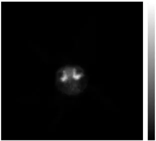
The data is modeled by several normal distributions in section 2.2. However, it is observed that the proportion of small pixel value is very large in all PET images. The main reason for this phenomenon is that luminosity of non-living parts in PET images is very weak but occupies large area. The region is called the background image. The following is an example of mouse brain. It shows that the histogram for pixels of a mouse brain.
Figure 2.3.1: It is the histogram for small pixels of a mouse brain in MicroPET image
The distribution of all background pixels tends to accumulate in the left in figure 2.3.1, and the peak is found when pixel value is zero. Therefore, the right-skewed distribution is considered to be the model of small pixels in PET image. Otherwise, we use mixed normal distribution to model non-background data. The model called flexible mixture model (FMM) is defined by 1 ( | ) ( | ) K i k k i k f x f x k
with 1 1 , 0 1 K k k k
, (2.3.1) and ( , 1 2,, K, 1, 2,,K),where fk(x |k) means the kth distribution. When k=1, the probability density function 1(x 1
fk |k )
K, fk
is skewed to right and it can be used to model the background image. When
k=2,…, (x |k) is the kth normal distribution where parameters are denoted by ( , )
k k k
and these mixture normal distribution can be used to model the non-background image. First the indicator function Yik is defined as
The concept is similar to G 1 , if comes from kth distribution.x
0 , otherwise. i ik Y (2.3.2)
using the EM algorithm in FMM MM. The main difference is 1(x | 1)
k k
f of the two models. The first let Yi (Yi1,,YiK), then joint probability density
i is function of xi and y 1 ( ,i i) ik k ( i| k) k f x y y f x K
. 1 2 ( , , , (2.3.3) The following derivation is similar to (2.2.8)~(2.2.30) for finding K1 2
, , , , )
K
such that is maximized. And becauseQ( ;
into two parts (2.2.20) and (2.2.21). First f ( ) ( ; old ) Q ( d))can be divided (new) k maximize ol
ormula (2.2.20) is considered and e result of (2.2.29). formula (2.2.20) in th ( ) ( ) ( ) ( ) ( ) 1 1 ) old i j j
part of formula (2.2.21) ( | ) 1 ( | old old N new k k i k k K old j i j f x N f x
. (2.3.4)At another , fk1(x |k1) skewing to the right is different from 1(x | 1)
k k
f in section 2.2. Here let fk1(x |k1) to be exponential distribution first. 1 1 1 1 ( | ) exp( ) , 0, 0 k k f x x x (2.3.5)
Formula (2.2.21) is simplified for obtaining the estimations of k ( ) ( ) ( ) ( ) 1 1 1 ( | ) log( ( | )) ( | ) old old N K k k i k k i k K old old i k j j i j j f x f x f x
(2.3.6)
( ) ( ) 1 1 1 1 ( ) ( ) 1 ( ) ( ) 2 2 2 2 2 2 2 2 ( ) ( ) 2 1 ( ) ( ) ( ) ( ) 1 ( | ) log ( | ) ( | ) 1 1 ( ) log 2 log 2 2 2 ( | ) ( | ) 1 log 2 2 ( | ) old old i i K old old j j i j j old old i i K old old j j i j j old old K K i K K old old j j i j j f x x f x f x x f x f x f x
1 2 2 2 ( ) 1 log 2 2 N i i K K K x
. (2.3.7)The three parameters ,kandkcontained in the parameter set k are considered for maximizing of formula (2.3.7). First, we partially differentiate with respect to,
Let ( ) ( ) 2 1 1 1 ( ) ( ) 1 1 ( | ) 1 0 ( | ) old old N i i K old old i j j i j j f x x f x
(2.3.8) ( ) ( ) 1 1 1 2 ( ) ( ) 1 1 ( | ) 0 ( | ) old old N i K old old i j j i j j f x x f x
i (2.3.9) ( ) ( ) ( ) ( ) 1 1 ( ) ( ) ( ) ( ) ( ) 1 1 ( | ) ( | ) = ( | ) ( | ) old old N k k i k i K old old i j j i j j new old old N k k i k K old old i j j i j j f x x f x f x f x
. (2.3.10)In addition, kmust be considered for obtaining the parameter set k such that formula (2.3.7) is maximized. Next, we partially differentiate with respect tok,
Let ( ) ( ) 2 ( ) ( ) 1 1 ( | ) 0 ( | ) old old N k k i k i k K old old i k j j i j j f x x f x
(2.3.11) ( ) ( ) ( ) ( ) ( ) ( ) ( ) ( ) 1 1 1 1 ( | ) ( | ) 0 ( | ) ( | )old old old old
N N
k k i k k k i k i K k K
old old old old
i i j j i j j j i j j j f x f x x f x f x
(2.3.12)( ) ( ) ( ) ( ) 1 1 ( ) ( ) ( ) ( ) ( ) 1 1 ( | ) ( | ) ( | ) ( | ) old old N k k i k i K old old i j j i j j new k N old old k k i k K old old i j j i j j f x x f x f x f x
. (2.3.13)Finally, we partially differentiate with respect tok, Let ( ) ( ) 2 2 2 2 ( ) ( ) 1 1 ( | ) 1 ( ) 0 2 2( ) ( | ) old old N k k i k i k K old old i k k j j i j j f x x f x
(2.3.14) ( ) ( ) 2 ( ) ( ) 1 1 2( ) ( ) ( ) ( ) ( ) 1 1 ( | ) ( ) ( | ) ( | ) ( | ) old old N k k i k i k K old old i j j i j j new k N old old k k i k K old old i j j i j j f x x f x f x f x
. (2.3.15)Partial derivatives of formula (2.3.6) with respect to,kandkare less than zero. It means the result of equation (2.3.10), of equation (2.3.13) and of equation (2.3.15) maximizes formula (2.3.6). So Q is maximized by the result of equations (2.3.4), (2.3.10), (2.3.13) and (2.3.15). After getting the estimations, use (2.2.48) as classification rule to determine how data points should be classified.
(new) (new) k (old) 2(new) k ( ; ) 1 ( | ) , arg max ( | ) k i k k i m k K j j i j j f x x G where m f x
. (2.3.16)FMM Clustering Algorithm (Exponential distribution and normal distribution mixture)
Step 1. Input data X { ,x x1 2,,xN}
Step 2. Decide the number of groups K, and give initial value(old) .
the new estimations (new).
Step 4. If , stop iterating with newly updated
estimates, else replace by new estimations and repeat step3. ( ) ( )
log (L new ) log ( L old )tolerance
(old)
Step 5. After iterations finish, use equation (2.3.16) to classify data points.
Gamma distribution with 1 is an exponential distribution, fk1(x |k1) is replaced by Gamma distribution. The derivation is similar to the derivation of using exponential distribution and normal distributions mixture model above.
1 1 1 1 exp( ) ( | ) , 0, 0, 0 ( ) k k x f x x x (2.3.17)
The estimation k(new) is obtained by result of equation (2.2.29). That is ( ) ( ) ( ) ( ) ( ) 1 1 ( | ) 1 ( | ) old old N new k k i k k K old old i j j i j j f x N f x
. (2.2.18)The estimation k(new)is still obtained by (2.2.21) and it is simplified as follows ( ) ( ) ( ) ( ) 1 1 1 ( | ) log( ( | )) ( | ) old old N K k k i k k i k K old old i k j j i j j f x f x f x
(2.3.19)
( ) ( ) 1 1 1 1 ( ) ( ) 1 ( ) ( ) 2 2 2 2 2 2 2 2 ( ) ( ) 2 1 ( ) ( ) ( ) ( | )log log ( ) ( 1) log
( | ) ( | ) 1 1 ( ) log 2 log 2 2 2 ( | ) ( | ) ( | old old i i i K old old j j i j j old old i i K old old j j i j j old old K K i K old j j i f x x x f x f x x f x f x f x
1 2 2 2 ( ) 1 ( ) 1 1 log 2 log 2 2 2 ) N i i K K K old K j j x
. (2.3.20)Where k contains the parameters ,,kandk. And the estimations , and are obtained by (2.3.10), (2.3.13), (2.3.15). Those are
(new) (new) k (new) k ( ) ( ) ( ) ( ) 1 1 ( ) ( ) ( ) ( ) ( ) 1 1 ( | ) ( | ) = ( | ) ( | ) old old N k k i k i K old old i j j i j j new old old N k k i k K old old i j j i j j f x x f x f x f x
. (2.2.21) ( ) ( ) ( ) ( ) 1 1 ( ) ( ) ( ) ( ) ( ) 1 1 ( | ) ( | ) ( | ) ( | ) old old N k k i k i K old old i j j i j j new k N old old k k i k K old old i j j i j j f x x f x f x f x
. (2.2.22) ( ) ( ) 2 ( ) ( ) 1 1 2( ) ( ) ( ) ( ) ( ) 1 1 ( | ) ( ) ( | ) ( | ) ( | ) old old N k k i k i k K old old i j j i j j new k N old old k k i k K old old i j j i j j f x x f x f x f x
. (2.2.23)The estimation is obtained as follows. First we partially differentiate formula (2.3.20) with respect to (new) . Let ( ) ( ) 1 1 1 ( ) ( ) 1 1 ( ) ( | ) log log 0 ( ) ( | ) old old N i i K old old i j j i j j d f x d x f x
(2.3.24)
1
0The th derivative of the Gamma function ( ) (ln )
( ) is : n x t n n d x t e t dt d n x
1 ( ) ( ) 1 1 1 0 ( ) ( ) 1 1ln
(
|
)
log
log
0
( )
(
|
)
t old old N i i K old old i j j i j jt
e
t dt
f x
x
f x
(2.3.25)It is difficult to solve the equation (2.3.25) for obtaining the estimation . Therefore, the concept of maximization step in generalized EM (GEM) algorithm and method of moment estimator (MME) are used to find estimation . First let the estimation by MME denote by (new) k (new) k ( ˆk MME )
. The estimation is found to have the maximum value of incomplete space log-likelihood for
(new
k
)
in a range of value and
. (2.3.26)
( ) ( ) ( ) ( )
ˆ (
new old old k k k MME k
)
In others words, the estimations , , , , by (2.3.18), (2.3.21), (2.3.22), (2.3.23) and (2.3.26) increase the incomplete space log-likelihood as much as possible. The algorithm is as follows.
(new) k (new) (new) k (new) k (new) k
FMM Clustering Algorithm (Gamma distribution and normal distribution mixture)
Step 1. Input data X { ,x x1 2,,xN}
Step 2. Decide the number of groups K, and give initial value(old) .
Step 3. Updated the estimations by equation (2.3.18), (2.3.21), (2.3.22), (2.3.23) and (2.2.26) to obtain the new estimations (new)
.
Step 4. If , stop iteration with newly updated
estimates, else replace by new estimations and repeat step3. ( ) ( )
log (L new ) log ( L old )tolerance
(old)
2.4 Kernel Density Estimation (KDE)
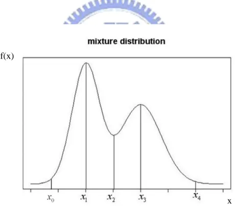
The issue of selecting initial values in GMM or FMM is solved by kernel density estimation (KDE) method [7]. The high and low peaks in kernel density curve are used for giving the initial values in KDE, and its bandwidth is determined by the program code of “density” in software R. Number of the high peaks is also used to select cluster size K. Therefore KDE method is considered before classifying the data. The concept of KDE is when data contains different structure from different distributions, the mixture distributions are used. First the kernel density curve is made by data and K high peaks are determined by kernel density. The definition between finding K different structures in data is the same. We give a basic example as follows
f(x)
x
Figure 2.4.1: The mixture distribution is composed of two normal mixture distributions, the mean is 1 and the standard deviation is 1 in one of normal mixture distributions, mean is2 and the standard deviation is 2 in another. It is observed that data contains two structures by kernel density. The data is actually generated from two normal distributions.
The model is normal mixture model, the high peaks can be estimated from the means of two normal distributions. That isˆ1 , x1 ˆ2 . And because 99% data of one structure comes x3
from normal distribution is contained in 6-standard deviation. In other words, maximum and minimum of 99% of the data from one structure between 6-standaed deviations are in the lower peaks. So the estimations of standard deviation are obtained by the above concept. That
is 1 0 1 ˆ 3 x x , 4 2 ˆ 3 3 x x
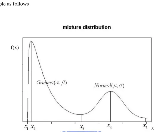
. But this method can not be used in FMM. We give a basic example as follows
f(x)
x
Figure 2.4.2: The mixture distribution is composed of Gamma( , ) and Normal( , ) .
We want to estimate and of Gamma distribution in Figure 2.4.2. Since most of the same structure is among the low peaks, we first find low peaks from kernel density curve such that data is separated as several structures. Then the low peaksx1andx3can be found in the structure of (Gamma , ). The initial values can be obtained by method of moment estimator (MME) for and from the low peaks x1 and x3 can be found in the structure of (Gamma , ). Finally, put the initial values into FMM to classify the data.
2.5 Model Selection
First the number of groups K must be decided before using K-means or GMM or FMM for further research. The choice of the number of groups is very important. The grouping results are always very different when we choose different numbers of groups. Model selection criterion like Akaike information criterion (AIC) or Bayesian information criterion (BIC) is useful to select the cluster size K [7]. They are defined as follows
2 log( ) 2
AIC L p (2.5.1)
2 log( ) log( )
BIC L p N (2.5.2)
p means the number of free parameters. L is maximum likelihood of the model estimated. N means the number of all data. The goal is selecting the number of groups K by finding p such that AIC or BIC minimizes. The value AIC and BIC are the same when the sample size
N is 7.389, and the penalty term in BIC is bigger than in AIC when the sample size N is bigger than 7.389. Therefore the BIC is preferred because pixel size in PET images are larger than 7.389. In other words, a simpler model can be selected with smaller numbers of groups by BIC.
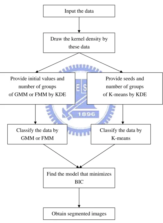
2.6 Procedure
The procedures of K-means with KDE, GMM with KDE and FMM with KDE are shown as follows.
Input the data
Draw the kernel density by these data
Provide initial values and number of groups of GMM or FMM by KDE
Provide seeds and number of groups of K-means by KDE
Classify the data by GMM or FMM
Find the model that minimizes BIC
Classify the data by K-means
Obtain segmented images
Figure 2.6.1: The procedure for segmentation of data by K-means with KDE, GMM with KDE and FMM with KDE
Chapter 3. Application
3.1 The PET Scanner
Positron emission tomography (PET) is a non-invasive nuclear medical scanning method. The effect of mutual destruction between positron and electron is used. The gamma ray which is generated by the above effect is measured. The image is composed by computers from the distributions of positron isotope in human organs. Then the metabolic rate per unit is calculated. The medicine 18FDG (18F-labelled deoxyglucose) is used before PET scanning because 18FDG is similar to the glucose which is absorbed by malignant tumor. If there is specific light region in PET scanning, it means abnormal situation may occur at this region. Therefore, the PET scanning helps doctors to determine the abnormal regions in the human body. It can also help doctors assess the effects of tumor treatment. This is one of the medical tools for finding tumor in the human body in recent years.
Furthermore, MicroPET is used to research on small animals like mouse. The main reason is that human disease behavior can often be modeled using small animals. Therapies of human diseases are based on analyzing physiological change. The slice of mouse brain in MicroPET images is shown as follows.
3.2 Phantom Study
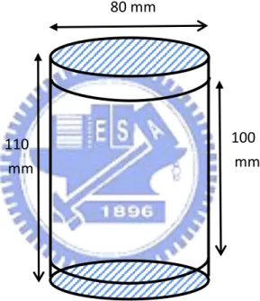
PET images can be used to find the abnormal regions in organisms as described in section 3.1. However, the region we discovered by clustering methods in PET images can not determine the abnormal structure of organisms. Hence the phantom experiment is designed for comparing the accuracies of these clustering methods. We use the cylindrical container with radius 40mm and height 110mm for the phantom experiment. The width of the clapboard which divided the container into four blocks evenly is 5mm.
80 mm
100 mm 110
mm
Figure 3.2.1: The geometric information of the cylindrical container
Cylindrical container is subdivided into four compartments, each containing substance of different concentration. The four regions show different brightness in the PET image of the phantom experiment. There are 63 slices where pixel size is 256 256 . Therefore the data size is 63 256 256 .
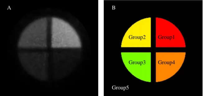
Group1 Group2 Group3 Group4 Group5 A B
Figure 3.2.2: (A) The 13thslice image of original MicroPET data in the phantom experiment. It is divided into four regions by the clapboard. Individual region shows different brightness. (B) The exact location of four different activities is known by the geometric information of the cylindrical container. The background image region is called Group5.
The highest activity region is defined as Group1, and the second-highest activity region is defined as Group2, and third highest activity region is defined as Group3, and fourth highest activity region is defined as Group4. Final the lowest activity region called background image is defined as Group5. We will use K-means with KDE, GMM with KDE and FMM with KDE to classify the original PET image data. The following figure is made by PET image data from the phantom experiment.
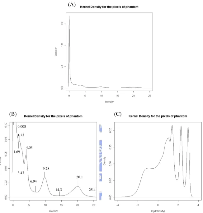
(A) (B) (C) 0.008 1.73 4.03 1.69 9.78 3.43 20.1 6.94 14.3 25.4
Figure 3.2.3: (A) The kernel density is made by the PET image data from the phantom experiment. (B) It is made by adjusting appropriate scope in x-axis and y-axis. The goal is to conveniently observe the peaks in kernel density and estimating the model parameters.
(C) Take log of data and then graph kernel density for more obvious peaks. These peaks are used because they are more obvious.
After selecting the initial values by KDE, the data is classified by the clustering methods in chapter 2. Since the grouping results are always very different because of differences about the number of groups, BIC is used to decide the numbers of groups.
(A) (B)
(C) (D)
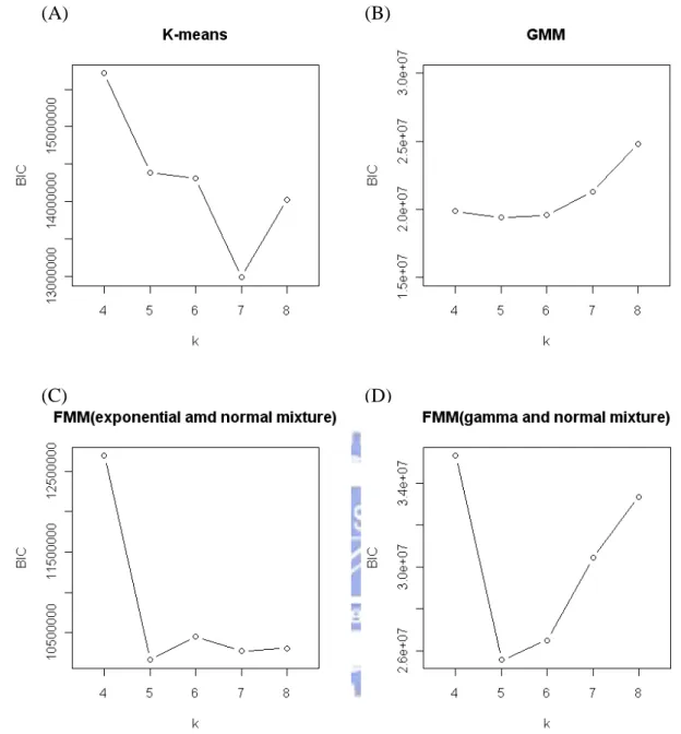
Figure 3.2.4: The BIC values are calculated from different models, k is the number of the groups. (A) K-means + KDE, when k=7 BIC is the minimum. (B)GMM + KDE, when k=5 BIC is the minimum (C) FMM (exponential and normal mixture) + KDE, when k=5 BIC is the minimum. (D) FMM (Gamma and normal mixture)+KDE, when k=5 BIC is the minimum.
It can be decided how to select the number of the groups by the result of Figure 3.2.4. Therefore, the following results are decided in the phantom experiment to classify the PET image data. Select k 7 when K-means with KDE is used, k 5 when GMM with KDE is used, k5 when FMM (exponential and normal mixture) with KDE is used and k5
when FMM (Gamma and normal mixture) with KDE is used. The images after different clustering methods show as follows.
A B
C D
Figure 3.2.5: (A) , the 13th slice image by K-means with KDE (B) , the 13th slice image by GMM with KDE (C)
7
k k5
5
k , the 13th slice image by FMM (exponential and normal mixture) with KDE (D) k 5, the 13th slice image by FMM (Gamma and normal mixture) with KDE
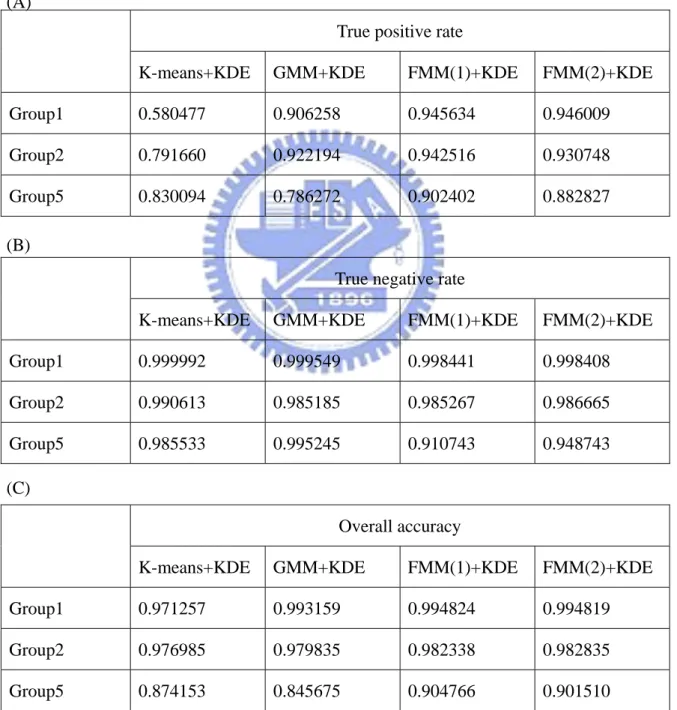
Figure 3.2.5 shows the 13th slice images with different clustering methods. It is observed that the clustering regions of Group1 and Group2 are a little different in (B), (C) and (D). However, since we are using different distributions for estimating the dark regions in PET image, the regions in Group5 are very different in (B), (C) and (D). The following table shows
three kinds of accuracy in Group1, Group2 and Group5.
Table 3.2.1: Compare the accuracy with four different methods from the result of Figure 3.2.5. Those methods are individual K-means with KDE, GMM with KDE, FMM(1) with KDE and FMM(2) with KDE. True positive rate shows in (A), negative rate shows in (B) and overall accuracy shows in (C).
Note: FMM(1) means exponential distribution and normal distribution mixture. FMM(2) means Gamma distribution and normal distribution mixture.
True positive rate
K-means+KDE GMM+KDE FMM(1)+KDE FMM(2)+KDE Group1 0.580477 0.906258 0.945634 0.946009 Group2 0.791660 0.922194 0.942516 0.930748 Group5 0.830094 0.786272 0.902402 0.882827 (A)
(B)
True negative rate
K-means+KDE GMM+KDE FMM(1)+KDE FMM(2)+KDE Group1 0.999992 0.999549 0.998441 0.998408 Group2 0.990613 0.985185 0.985267 0.986665 Group5 0.985533 0.995245 0.910743 0.948743 (C)
Overall accuracy
K-means+KDE GMM+KDE FMM(1)+KDE FMM(2)+KDE Group1 0.971257 0.993159 0.994824 0.994819 Group2 0.976985 0.979835 0.982338 0.982835 Group5 0.874153 0.845675 0.904766 0.901510
The accuracy of K-means with KDE is low in Group1, Group2 and Group5. The accuracy of GMM with KDE in Group1 and Group2 is a little better but it is still low in Group5. FMM(1) and FMM(2) are common in using the right-skewed distribution to be the model of background images. Hence the accuracy of FMM(1) or FMM(2) in Group1, Group2 and Group5 is significantly better than K-means or GMM. For Group3, FMM(1) is better than FMM(2). It is because the profile in FMM(1) can be observed clearly from Figure 3.2.5, but that in FMM(2) can not.
3.3 CT Study
In addition to PET images, we would like to apply these clustering methods to the other kind of data. Here we consider computerized tomography (CT) images. CT scanning is also one of the medical diagnosis tools using X-ray. It shows clearly the organization of organisms through a slice of image by X-ray absorption. The region of higher pixel value is lighter at the parts of high absorption, and the region of lower pixel value is darker at the parts of lower absorption. Comparing CT images and PET images, it is observed that it is easier to find the location of abnormal regions in the human body by PET images, and it is easier to outline by CT images. They are shown as the following figures.
A B
Figure 3.3.1: The 2D CT image is shown and there are 390 slices. (A) The 161 th slice PET image (B) The 161 th slice CT image
The profile and organ inside the body is very clearly from the CT image by Figure 3.3.1. Hence the result of segmentation for CT image is compared to original data by this feature. The other CT image whose size is 512 373 is used. Then the kernel density is made by this data for finding initial values.
A
(B)
Figure 3.3.2: (A) The sagittal plane in the CT image contains teeth, spine, trachea, etc. The data size is512 373 . (B) The kernel density is made by the pixel data in (A).
Next the BIC is used to select the numbers of groups k. It is shown the relationship between BIC and the numbers of groups k is as follows
(A) (B)
(C) (D)
Figure 3.3.3: The BIC values are calculated from different models; k is the number of groups. (A) K-means + KDE, when k=9 BIC is the minimum. (B)GMM + KDE, when k= 7 BIC is the minimum (C) FMM (exponential and normal mixture) + KDE, when k=9 BIC is the minimum. (D) FMM (Gamma and normal mixture) + KDE, when k=7 BIC is the minimum.
3.3.3. Therefore, select when K-means with KDE is used, when GMM with KDE is used, when FMM (exponential and normal mixture) with KDE is used and when FMM (Gamma and normal mixture) with KDE is used. The images after different clustering methods are,
9 k k 7 9 k 7 k A B C D
Figure 3.3.4: (A) k9, the image after using K-means with KDE (B) , the image after using GMM with KDE (C) , the image after using FMM (exponential and normal mixture) with KDE (D) , the image after using FMM (Gamma and normal mixture) with KDE 7 k 9 k 7 k
The trachea in the segmentation of the CT image is clear in Figure 3.3.4 (C) and Figure (D). They both are results of using right-skewed distribution and normal distribution mixture model. That is the FMM method. The K-means result in Figure 3.3.4 (A) is poor in the region of trachea. There are two groups in trachea. GMM also has two groups in trachea, as shown in Figure 3.3.4 (B).
Chapter 4. Conclusion
The methods of K-means with KDE, GMM with KDE and FMM with KDE are used to classify the data of PET images and CT images. It is observed that the FMM method has high accuracy in the high-activity region in PET images from Chapter 3. The accuracy of low-activity region from FMM is higher than that from K-means or GMM in PET images. The CT image is also clustered by these methods. The result of FMM is better than that of K-means or GMM in the lower pixels of data. After comparing these methods, the data of the PET images or CT images can be classified by FMM because the high accuracy of segmentation obtained by FMM in high and lower activity regions.
The FMM method considers the property and structure of data. It constructs a model to fit the original data more closely. Therefore, the result we obtained from FMM is better than GMM. We used exponential distribution with normal distribution mixture model and Gamma distribution with normal distribution mixture model. For further work, one can test and attempt to find more suitable distributions to increase the accuracy of data classification. Otherwise, the block of pixel values can be used to make pixel data to have more information, like the pixel location. So we can take multivariate normal distribution to model the original data, and compare the results by block method with one pixel point.
References
[1] Akaike H. Anew look at the statistical model identification. IEEE Trans. Automat. Ontr., 1974, AC-19, 716-723
[2] David W. Townsend, Jonathan P.J. Carney, Jerry T. Yap, Nathan C. Hall. PET/CT Today and Tomorrow. The Journal of Nuclear Medicine, Vol. 45, pp. 4S-14S, 2004.
[3] Hsiao IT, Rangarajan A, Gindi G. Joint-Map Reconstruction/Segmentation for transmission Tomography Using Mixture-Model as Priors. Proc. IEEE Nuclear Science Symposium and Medical Image Conference, 1998, 3, 1689-1693.
[4] Hung-Yuan Chiang. Segmentation of Dynamic MicroPET Images by K-mean and Mixture Methods. Master’s thesis, institute of Statistics National Chiao Tung University, 2004.
[5] McLachlan GJ, Bean RW, Peal D. A mixture model -based approach to the clustering of microarray expression data. Bioinformatics, 2000, 18, 3:413-22.
[6] Olinger JM, Fessler JA. Positron-emission tomography. EEE Signal Processing
Magazine, 1997, 41, 1, 43-55.
[7] Tai Been Chen. Statistical Applications of Maximized Likelihood Estimates with the Expectation-Maximization Algorithm for Reconstruction and Segmentation of MicroPET and Spotted Microarray Images. PhD’s thesis, institute of Statistics National Chiao Tung University, 2007.
[8] Vardi Y, Shepp La, Kaufman L. A statistical model for positron emission tomography.