An Ordinal Optimization Theory-Based Algorithm
for Solving the Optimal Power Flow Problem
With Discrete Control Variables
Shin-Yeu Lin, Yu-Chi Ho, and Ch’i-Hsin Lin
Abstract—The optimal power flow (OPF) problem with discrete
control variables is an NP-hard problem in its exact formula-tion. To cope with the immense computational-difficulty of this problem, we propose an ordinal optimization theory-based algo-rithm to solve for a good enough solution with high probability. Aiming for hard optimization problems, the ordinal optimization theory, in contrast to heuristic methods, guarantee to provide a top % solution among all with probability more than 0.95. The approach of our ordinal optimization theory-based algorithm consists of three stages. First, select heuristically a large set of candidate solutions. Then, use a simplified model to select a subset of most promising solutions. Finally, evaluate the candidate promising-solutions of the reduced subset using the exact model. We have demonstrated the computational efficiency of our algo-rithm and the quality of the obtained solution by comparing with the competing methods and the conventional approach through simulations.
Index Terms—Discrete control variables, nonlinear
program-ming, optimal power flow, ordinal optimization.
NOMENCLATURE
-dimensional vector of discrete con-trol variables such as switching shunt capacitor banks and transformer taps.
-dimensional vector of continuous variables consisting of real and reactive power generation, real and imaginary parts of bus complex voltage.
Sample space of .
Real and reactive power flow balance equations.
Inequality constraints such as thermal-limit security constraints, security thermal-limits on voltage magnitude, and real and re-active power generation limits.
Manuscript received March 11, 2003. This work was supported in part by the National Science Council, Taiwan, R.O.C., under Grant NSC91-2213-E-009-070, in part by the U.S. Army Contract DAAL03-92-G-0115 and Contract DAAH04-95-0148, in part by the Air Force under Grant F49620-98-1-0387, and by the Electric Power Research Institute under Contract WO8333-03.
S.-Y. Lin is with the Department of Electrical and Control Engineering, National Chiao Tung University, Hsinchu 300, Taiwan, R.O.C. (e-mail: [email protected]).
Y. C. Ho is with the Division of Engineering and Applied Sciences, Harvard University, Cambridge MA 02138 USA.
C.-H. Lin is with the Department of Electronics Engineering, Kao Yuan In-stitute of Technology, Kaoshiung, Taiwan 700, R.O.C.
Digital Object Identifier 10.1109/TPWRS.2003.818732
Objective function such as the total power generation cost or the total system losses.
MDCP Mixed discrete-continuous nonlinear optimization problem such as the op-timal power flow (OPF) problem with discrete control variables.
mixed discrete-continuous nonlinear optimization problem (MDCP) for a given .
Representation of a typical objective function in ordinal optimization theory. Continuous version of .
Lower and upper limit of . The component of and .
CP Continuous nonlinear optimization
Problem formed by replacing in MDCP with .
Local optimal solution of continuous nonlinear optimization problem (CP). The component of .
Nearest discrete value of to on the right-hand (left-hand) side of .
or .
Deviation of optimal objective value caused by .
Lagrange multiplier associated with at the optimal solution of CP.
Partial derivative of w.r.t.
evaluated at .
Partial derivative of w.r.t.
evaluated at .
Deviation of optimal objective value of CP due to the change of from to
.
Representative set of . Number of samples in .
SS Selected subset or estimated good
enough subset which consists of the estimated top % samples of . Number of samples in SS.
Approximate solution of
.
Number of top samples in SS ordered by the objective values of the quadratic approximate solutions of
that are guaranteed to consist of a good enough solution of MDCP.
I. INTRODUCTION
T
HE OPF problem has a long history in power-system research. Numerous numerical techniques had been developed for this problem such as the successive linear programming method [21]–[23], successive quadratic program-ming (SQP) method [4], [6], [26], Lagrange Newton method [19], [24], [25], the interior point method [28]–[30], and the re-cent dual-type method [11], [12], [14]. However, these methods are designed for purely continuous-variable OPF. In reality, the power systems consist of several discrete control variables such as the switching shunt capacitor banks, which are switched on and off in order to correct the voltage profile and reduce active power transmission losses and transformer taps, which are adjusted step by step to ensure that a voltage-controlled bus maintains its voltage within acceptable limits. In most of the existing OPF algorithms including the above-mentioned ones, discrete controls are treated as continuous variables until they are approximately optimized. Then they are rounded off to their nearest discrete values. Simply rounding off discrete controls can cause a considerable increase of the objective value and/or violations of inequality constraints. This defi-ciency had been recognized by Tinney et al. in [27]. A linear programming-based method was developed in [2] to deal with this type of mixed discrete-continuous nonlinear programming problems; however, it is too time consuming.To cope with the computational intractability and the disad-vantages induced by arbitrarily rounding off technique, a pe-nalized discretization algorithm is proposed by Liu et al. in [15]. They employed a complicated six rules to introduce the quadratic limit penalty of a discrete control during the solution process of a Newton OPF. They finally fix the penalized contin-uous discrete-control at its discrete value based on a local con-vergence criteria. In other words, they proposed a rounding off technique based on a penalized discretization. Thus, this method cannot completely resolve the problem of infeasibility caused by not treating the discrete control variables in their exact form. To solve the OPF with discrete control variables in a more exact manner, Bakirtzis et al. proposed an enhanced genetic algo-rithm (GA) in [1], which needs only the power flow solutions for fitness evaluation, however, sacrificing the hard restriction on branch flow limits. Thus, violations of inequality constraints may occur in this method. Recent methods that treat the discrete control variables in their exact form and take the feasibility of OPF into account are the mean field theory-based annealing al-gorithm [5], the evolutionary alal-gorithm [17], and the tabu search method [9]. However, these methods use global searching tech-nique, which is very computationally time-consuming provided that the size of the search space is huge.
To retain the merits of the above three methods in handling the discrete control variables and the feasibility of OPF while avoiding their immense computational-complexity, we intend to use the ordinal optimization (OO) technique, which is recently developed by Ho and his colleagues [7], [8]. This optimization technique can effectively reduce the number of search samples of the huge sample space formed by all discrete control variables and seek a good enough solution with high probability instead of searching the best for sure. Thus, the purpose of this paper
is to propose an OO theory-based algorithm to solve for a good enough solution of the OPF with discrete control variables effi-ciently. The approach of our algorithm consists of three stages. First, select heuristically a large set of candidate solutions. Then, use a simplified model to select a subset of most promising so-lutions. Finally, evaluate the candidate promising-solutions of the reduced subset using the exact model.
Since OO is a rather new optimization technique, we will in-clude some relevant materials in the appendices for easier ref-erence. Thus, our paper is organized in the following manner. In Section II, a mathematical formulation of the OPF problem with discrete control variables will be presented. In Section III, we will present our approach based on the OO theory to solve for a good enough solution of the OPF problem with discrete con-trol variables. In order not to affect the fluency of presentation, a detailed review of the OO theory [7], [8], the applications of the alignment probability [10] to our problem and a comment for addressing the question regarding infeasible solutions are given in Appendices A, B, and C, respectively. In addition, an efficient dual-type method for solving a set of quadratic programming problems, which are induced from our approach as stated in Sec-tion III, is presented in Appendix D. We concluded SecSec-tion III by presenting an online algorithm for obtaining a good enough solution of the OPF problem with discrete control variables. The test results and the comparisons of our online algorithm with the conventional approach and the competing methods on the IEEE 118-bus system and the IEEE 244-bus system are presented in Section IV. Finally, we make a conclusion in Section V.
II. MATHEMATICALFORMULATION OF THEOPF PROBLEM
WITHDISCRETECONTROLVARIABLES
The OPF problem with discrete control variables is a type of MDCP, which can be formulated as
subject to
(1) This optimization problem is to find the continuous and dis-crete control settings so as to minimize the objective function while satisfying the required constraints.
We can rewrite the MDCP shown in (1) as
(2) where we denote the optimization problem inside the bracket
for a given as , that is
(3) In convention and practical applications of power systems, a local solution of the OPF is usually sought. However, in the MDCP shown in (2), we can tell that even if we require a local solution only, we still need to solve the for all sam-ples . Thus, suppose each discrete control variable has p possible discrete values, then there will be samples in the
sample space . To give a flavor of the numerical value of the size of , assuming , and , there will be samples in . Therefore, it will be computation-ally intractable to solve for a local optimal solution of MDCP shown in (2) using a global searching technique.
III. OO THEORY-BASEDAPPROACH
Denoting the optimal objective value of the optimization problem for a given as a function of , say , then (2) becomes which has exactly the same form as the optimization problem treated in OO theory [7], [8]. Before stating our approach for the MDCP in (2), we will briefly state the idea of OO theory in the following while the details are given in Appendix A.
A. Review of OO Theory
The OO theory is a new methodology designed to cope with hard problems such as the lack of structure problems, prob-lems with uncertainties, or probprob-lems with huge sample space that grows exponentially with respect to the problem size. The problem considered in this paper is of the latter kind. There are two basic tenets of the OO theory. The first is that of order versus value in decision making. It is obvious that determining whether is much easier than determining : consider the intuitive example of deter-mining which of the two boxes in two hands is heavier versus identifying how much heavier one is than the other. The second tenet is the goal softening. Instead of asking the best for sure in optimization, it settles for the good enough with high proba-bility. A conclusion drawn from the OO theory is the following. Suppose we simultaneously evaluate a large set of alternatives very approximately and order them according to the approxi-mate evaluation. Then there is high probability that we can find the actual good alternatives if we limit ourselves to the top % of the observed good choices.
Thus, first, we use only a very rough model to order the good-ness of a solution relying on the robustgood-ness of ORDER against noise and model error to separate the good from the bad. Second, we soften the goal of the problem and look for a good enough solution, which is among the top % of the search space , with high probability. These two steps greatly reduce the com-putational burden and search difficulties of the problem as will be detailed in Appendix A. A summary of these search proce-dures for obtaining a good enough solution of
with high probability can be described in the following: i) Using either a uniform selection or a heuristic method to se-lect a representative set with size N, say 1000, for the search space . ii) Using an easily computed crude model to roughly evaluate and order the performance of each sample in and collect the top s samples to form a selected subset (SS), which is the estimated good enough subset. The OO theory guar-antees that SS consists of actual good enough solutions with high probability. The value of in our approach determined based on the alignment probability [10] is 50 as will be de-scribed in Appendix A.II. iii) Evaluating the objective value of the for each sample in SS to obtain the good enough solution.
B. Three-Stage Approach
Based on the above search procedures, our three-stage ap-proach for obtaining a good enough solution of the MDCP shown in (2) is presented in the following.
i) Using a heuristic method to determine the set . First, we define the MDCP shown in (2) as a contin-uous nonlinear optimization problem (CP) if we replace the discrete as continuous . Thus, the resulting CP is shown in (4)
(4) Our strategy to determine the set is to solve the CP to obtain an optimal solution first. Then, we can set each component of the discrete , say , be either or . At this stage, we have reduced the search space from to . In fact, this is a similar intuition as the conventional approach for solving the MDCP in (2), because we believe that good solutions should be among the samples. However, arbitrarily rounding off does not guarantee a good enough solution with high probability. In general , we need to reduce the search samples further. To do so, we will estimate the deviation of the optimal
objective value caused by that is
, where
in which , if , and
. Based on the sensitivity theorem in [16], we can obtain
(5) Now if , a predetermined small posi-tive real number, then we fix the discrete at if or if . In other words, if is set to be (or ) and the es-timated deviation of the objective value is small, then we fix at (or ). Suppose there are fixed by this manner, there will be components of not yet fixed. Thus, we have further reduced the search sam-ples from to . The value is selected so that . The above process constitutes our heuristic method for determining the set .
ii) Determining the selected subset (SS) based on a crude model.
Now let us denote the N samples in as . To pick out the samples to form SS, we will employ a crude model, which estimates the deviation of the optimal objective value in (4), that is , due to the change of from to . The formula for es-timating is an extension of the formula of (5) by considering the vector increment
rather than the component increment and is stated in the following:
We order the samples in based on ob-tained from (6) as follows. The sample with lower value of , that is the sample being less sensi-tive to the optimal objecsensi-tive value of (4), will be ranked higher. In other words, the samples, which are likely to retain the optimal objective value of (4) are ranked higher. Consequently, the top ranked form SS, where denotes the size of SS determined based on the alignment probability [10] as will be detailed in Ap-pendix I. The SS thus formed is the estimated good enough subset. Now according to the OO theory [7], [8], SS consists of actual good enough samples with high probability.
iii) Finding the Good Enough Solution. Let us denote the samples in SS by
. Suppose we solve the exactly for each sample in SS, the sample that has the least objective value will be the good enough solution that we are looking for as have been concluded by the OO theory [7], [8]. However, solving s , which are nonlinear constrained optimization problems, is too time consuming to meet the requirement of online power system operation. Thus, to resolve this computa-tional difficulty, we employ a two-phase strategy based, again, on the OO theory [7], [8]. Before presenting this two-phase strategy, a tough question that may be raised is what if all s samples in SS are infeasible? We have addressed this question in Appendix C.
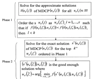
Now as shown in Fig. 1, the basic idea of our two-phase strategy is to evaluate the s samples in SS very approximately first and order them according to this approximate evaluation. Then, the actual best alternative will be contained in the top few observed good choices. Thus, in phase 1, we can efficiently solve for the approximate solutions of the s
and order them based on their corresponding objective values, which represent the estimated performance of the s . Then, in phase 2, we only solve for the exact solutions of the for the few top ranked sam-ples obtained in phase 1, and the one with least objective value is the good enough solution that we look for. In the following, we will describe this two-phase approach in detail. In the first phase, we will solve the
approximately for a given by solving its quadratic approximate problem as shown in the following:
(7) where is an identity matrix, and is a small posi-tive scalar but enough to make the Hessian of (7) posiposi-tive definite.
Fig. 1. Two-phase strategy for finding the good enough solution.
We let denote the optimal solution of (7), then is the approximate solution of the optimization problem inside the bracket of (2) for
. We have developed an efficient dual-type method called DPPQN in [11], [12], [14], which is especially suited for solving (7) for all samples . However, in order not to affect the fluency of presentation, we will present this method in Appendix D. Furthermore, this dual-type method can also re-solve the computational difficulty caused by the infeasibility of (7) for a given . Since the practical objective func-tions of the OPF such as the total generation cost and the total system losses are mostly convex, the quadratic-approximated shown in (7) should be a good approximate model of the actual , thus the order of
ordered based on the objective value should be closely related to the order of , ordered
based on the objective value .
Therefore, we can estimate the number of top ranked sam-ples in that will consist of the actual top sample based on the alignment probability [10]. That is,
to estimate the such that .
Once is estimated, we need only to solve the exact solution of
for . In our problem,
and the detailed procedures for obtaining based on the align-ment probability [10] are described in Appendix B.
C. OO Theory-Based Algorithm for Solving the MDCP
Now, we are ready to state our algorithm for solving the MDCP shown in (2) to obtain a good enough solution.
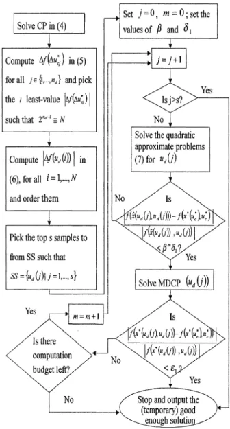
Step 1) Solve the CP in (4) using the method proposed in [11], [12] to obtain .
Step 2) Compute by (5) for each
and . Pick the least-value , such that , then set
to be if , or if
Steps 1 and 2 is how we pick the N samples needed for ordinal optimization.
Step 3) Compute by (6) and calculate
for all .
Step 4) Rank all N samples based on their values of obtained in Step 3, such that the sam-ples with smaller will be ranked higher. Then pick out the top samples to form SS. Steps 3 and 4 use a very crude model to form the selected subset (SS) required by OO theory. Step 5) Solve (7) for all in SS using the dual
pro-jected pseudo Quasi-Newton (DPPQN) method described in Appendix D to obtain the
approx-imate solutions . Order
the s based on their approximate
objec-tive values ,
to be , such that if
,
then .
Step 6) Find the exact solutions of the in (3) for , obtained in Step 5. The one having the least objective value is the good enough solution.
Step 5 uses a slightly more accurate but still approx-imate model to evaluate the few top-ranked sam-ples obtained in Step 4. OO theory then guarantees that the best ranked sample in Step 6 is indeed good enough with high probability.
D. Online Modifications
It is quite possible that before completing the solution process of solving the quadratic programming problems shown in (7) for all samples in SS, we may already obtain an approximate solution whose objective value is close to . Considering the limited computation budget for online optimal power flow ap-plication, we should solve for the exact solution of
for this sample immediately instead of solving it after all s quadratic approximate solutions are obtained. Consequently, if the objective value of the resulting solution of this sample is close to , we have obtained a good enough solution. Otherwise, we will go on for the next sample. Such a modification definitely saves computational time. Thus, we can modify steps 5 and 6 of our algorithm presented in previous subsection for online applications as follows.
Step 5M: Set and set ; set the values of and ; set the non-negative
integer .
Step 6M: Solve (7) for . If
,
solve the for this to obtain
and go to Step 7M; otherwise, set . If , repeat this step; otherwise, go to Step 8M.
Step 7M: If
, where is a small positive real number, then
Fig. 2. Flowchart of proposed online algorithm.
is the good enough solution
and stop; otherwise, set as
the temporary good enough solution and check whether there are enough computation budget left; if not, stop and output the temporary good enough solution; otherwise, go to Step 8M. Step 8M: If , stop and output the temporary good
enough solution; otherwise, set and return to Step 6M.
With the above modifications, we show the flowchart of our OO theory-based online algorithm in Fig. 2. In addition, a brief illus-tration about the parameters and is given in the following remark.
Remark 1: The positive real number in Step 6M is used to measure the closeness between
and . Thus, in Step 5M, we can set to be a not too small value, say 0.03, so as to obtain a temporary
good enough solution in Step 6M fast.
Subsequently in Step 7M, if is close
enough solution that we are looking for; otherwise, we will increase m by 1 in Step 8M and return to Step 6M. When m increases, will decrease, because behaves like a reduction factor. Thus, we can proceed further to obtain a better temporary good enough solution or the good enough solution. We typically set in Step 5M.
IV. TESTRESULTS
A. Test Systems and Test Cases
We have tested our online algorithm on the OPF problems with discrete control variables of the IEEE 118-bus system and the IEEE 244-bus system [30]; the former consists of 18 gen-eration buses and 179 transmission lines, and the latter consists of 47 generation buses and 445 transmission lines. It should be noted that the values of conductance of the transmission lines in the IEEE 244-bus system are much higher than that of the IEEE 118-bus system on the average. We consider two types of objective function: the minimum total real power generation
cost and the minimum system losses
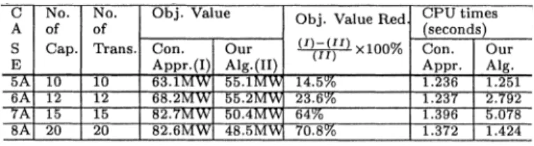
, where denotes the real power generation of gen-eration bus , and are generation cost coefficients, and denotes the real power loss on transmission line . For each system and each objective function, we have tested several cases associated with various number of capacitors and various number of transformers. We assume each capacitor is equipped with three capacitor banks, and the capacity of a bank ranges from 14 to 42 MVAR. We assume each transformer tap has 32 discrete steps such that each step is 5/8% of the nominal trans-former tap ratio. A summary of all the test cases is described below. Case 1A to Case 4A in Table I and Case 5A to Case 8A in Table II represent the test cases on the IEEE 118-bus system. Case 1A to Case 4A use the total generation cost, while Case 5A to Case 8A use the total system losses as their objective functions. The number of capacitors and the number of trans-formers assumed in Case 1A–8A are shown in the second and third columns of Tables I and II. Case 1B to Case 4B in Table III and Case 5B to Case 8B in Table IV represent the test cases on the IEEE 244-bus system. Case 1B to Case 4B use the total generation cost, while Case 5B to Case 8B use the total system losses as their objective functions. The corresponding number of capacitors and transformers assumed in these eight cases are also shown in the second and third columns of Tables III and IV. It should be noted that all the tests we have made are carried out in a Pentium IV personal computer.
B. Comparison With the Conventional Approach
Our tests for demonstrating the performance of our online al-gorithm in comparison with the conventional approach are car-ried out in the following. We first solve these 16 cases using the conventional approach, which solves the CP in (4) for each case first then round the obtained optimal continuous values of the discrete control variables, , off to their nearest dis-crete values. After the values of the disdis-crete control variables are fixed at the nearest , we then solve the , and the resulting objective values and the consumed CPU times are shown in the fourth and the seventh column, respectively, of each table. We apply our online algorithm presented in
Sec-TABLE I
COMPARISON OFOURONLINEALGORITHMWITH THECONVENTIONAL
APPROACH ONCASES1A–4AOF THEIEEE 118-BUSSYSTEMUSING THE
TOTALGENERATIONCOST AS THEOBJECTIVEFUNCTION
TABLE II
COMPARISON OFOURONLINEALGORITHMWITH THECONVENTIONAL
APPROACH ONCASES5A–8AOF THEIEEE 118-BUSSYSTEMUSING THE
TOTALSYSTEMLOSSES AS THEOBJECTIVEFUNCTION
TABLE III
COMPARISON OFOURONLINEALGORITHMWITH THECONVENTIONAL
APPROACH ONCASES1B–4BOF THEIEEE 244-BUSSYSTEMUSING THE
TOTALGENERATIONCOST AS THEOBJECTIVEFUNCTION
TABLE IV
COMPARISON OFOURONLINEALGORITHMWITH THECONVENTIONAL
APPROACH ONCASES5B–8BOF THEIEEE 244-BUSSYSTEMUSING THE
TOTALSYSTEMLOSSES AS THEOBJECTIVEFUNCTION
tion III-D with , and to solve for
a good enough solution for each case, and the resulting objec-tive value and the consumed CPU times are shown in the fifth and the eighth column, respectively, of each table. The reduction of the objective values achieved by our online algorithm com-pared with the conventional approach is given in column 6 of each table. We found that among all of the discrete control vari-ables, the objective value (4) is less sensitive to transformer tap ratio changes than it is to the capacitor bank changes; hence, we set the transformer tap ratios fixed in Step 2 of our online algo-rithm. This result is consistent with the observation in [15]. The values of the discrete control variables obtained by the conven-tional approach may be infeasible as appeared in Cases 4A, 1B, and 2B in which infinite objective values are indicated; how-ever, our online algorithm obtains good enough solution in all cases we have simulated. This demonstrates the probability of
not obtaining any feasible solution by our algorithm is extremely low comparing with the conventional approach. Furthermore, the CPU times consumed by our online algorithm is slightly larger than that consumed by the conventional approach in most of the cases as can be observed from the last two columns of all tables. Thus, compared with the conventional approach, we ob-served that: i) our online algorithm is also suitable for real-time application; ii) the improvements on the objective values for ei-ther the minimum total generation cost or minimum total system losses are 28% on the average; and iii) we can always obtain a good enough solution in contrast to the possible failure of the conventional approach.
C. Comparison With the Competing Methods
Our method deals with the OPF problems with discrete con-trol variables in their exact form and takes the feasibility of OPF into account in contrast to the penalized discretization algo-rithm [15] and the enhanced genetic algoalgo-rithm [1]. Thus, we can avoid any possible ambiguity on the feasibility of our solution. The recent methods that treat the discrete control variables and the feasibility of OPF like our algorithm are mean-field theory based annealing algorithm [5], the evolutionary algorithm [17], and the tabu search method [9]. However, these methods are seeking the global optimal solution of the OPF (2) within the huge sample space , which should be very computationally time consuming. For examples, the mean field theory-based an-nealing algorithm took 10 min to solve the OPF of a 270-bus system as reported in [5], and the tabu search method and evo-lutionary algorithm took 6 and 27 min, respectively, to solve the OPF of a 24-bus system as described in [9]. In fact, the com-putational complexity caused by global searching technique is what our OO theory-based online algorithm intend to resolve by seeking a good enough solution with high probability instead.
To demonstrate the merits of our online algorithm, we should compare with the above mentioned methods by simulations. In [5], the mean field theory-based annealing algorithm compared only with the SQP method for a four-bus and 30-bus systems. However, the tabu search method in [9] had compared with and beaten the evolutionary algorithm and the SQP method. Thus, it would be typical to compare our online algorithm with the tabu search method.
The tabu search is an iterative algorithm; it starts from a randomly generated feasible solution and moves to a better so-lution in the randomly selected neighborhood by the following procedures. Starting from the best solution in the selected neighborhood, if it does not belong to the Tabu List (TL), or in case of being in the TL but passes the aspiration level (AL) test, it will be added to the TL and a move to this solution will be carried out; otherwise, repeat these procedures for the next best solution. During the search process, the best solution is always updated and stored aside until the stopping criterion is satisfied. Details of this method can be found in [9] and [18]. We apply the tabu search method to all of the cases shown in Tables I to IV. Due to the page limitation, we cannot present all of the comparison results. However, we will show some typical cases to demonstrate the efficiency of our online algorithm. Figs. 3–6 describe the simulation results of applying our online algorithm and the tabu search method to Cases 5A, 7A, 5B,
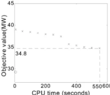
Fig. 3. Comparison of our online algorithm and the tabu search method on Case 5A.
Fig. 4. Comparison of our online algorithm and the tabu search method on Case 7A.
Fig. 5. Comparison of our online algorithm and the tabu search method on Case 5B.
Fig. 6. Comparison of our online algorithm and the tabu search method on Case 7B.
and 7B. The objective functions of these four cases are the minimum system losses. In each of the four figures, the point marked by “x” denotes the pair of the objective value of the best solution so far and the corresponding consumed CPU times during the search process of the tabu search method applying to the corresponding case. However, the point marked by “o” in each figure denotes the pair of the objective value of the final solution and the corresponding CPU times obtained
by our online algorithm. We let denote the coor-dinate of point “o”, where represents the corresponding case. From column 8 and column 5 of Tables II and IV, we see that
, and
. We let denote
the coordinate of the specific point “x”, such that
in the corresponding case . We also mark in each figure, that is
, and . From Figs. 3–6, we see that the improvement of the solution during the search process of the tabu search method is very sluggish. Even when tabu
search method consumes CPU times, is
still at least 18% more than in each case. These results demonstrate the efficiency of our online algorithm in getting a good enough solution.
V. CONCLUDINGREMARKS
The OPF problem with discrete control variables is an NP hard problem and has a long history in power system research. In this paper, we have developed an OO theory based online al-gorithm to deal with it. We treat the discrete control variables in their exact form and take the feasibility of the OPF into ac-count. Our online algorithm can get a good enough solution of the considered problem efficiently to resolve the computational complexity caused by the approach of global searching tech-niques such as the mean field theory-based annealing algorithm [5], evolutionary algorithm [16], and the tabu search method [9]. We have demonstrated the computational efficiency of our on-line algorithm and the quality of the obtained solution by com-paring with the tabu search method and the conventional ap-proach through simulations.
Above all, our ordinal optimization theory-based algorithm has a very important implication in power system control and management, because most of the power system optimization problems involve discrete control variables; a popular example problem in addition to the current one is the optimal capacitor placement problem.
APPENDIX A
I. OO Theory [7], [8]
In order to make the computation of the NP hard problem tractable, where is a nonstructured huge sample space, the OO theory soften the goal from the best for sure to good enough with high probability such that a great reduction of the search space can be achieved. To proceed with the search reductions, the OO theory starts from defining a rep-resentative set of , denoted by , which can be obtained by either a uniform selection or a heuristic method. Usually, the size of , denoted by N, is sufficiently large, say 1000. A Good Enough Subset of , denoted by , is formed by the top ranked %, say , samples of . As shown in [13], with a very high probability 0.991, where denotes the Good Enough Subset of formed by the top %, say , samples of . Thus, to seek a good
enough solution of , it is sufficient to seek a good enough solution of . However, a is easy to specify but diffi-cult to obtain; for example, in our problem, one needs to solve , that is N nonlinear constrained op-timization problems, to determine the which is, of course, computationally intractable for large power systems. Thus, to reduce the search samples while obtaining members in , the OO theory advocates the use of a very crude model in eval-uating the “goodness” of any proposed solution sample. Using such a crude model one can with manageable effort estimate what are the top % of the samples. Call this estimated top % the Selected Subset (SS). In other words, the SS is determined by first ranking the samples in based on an easily computed
crude model of noted by , where denotes
the modeling noise or error, then choose the top samples to form SS. The OO theory then provides a universal alignment probability between the intersection of the and the SS [10]. Furthermore, OO theory provides in [10] a formula for obtaining the value as the value of a six-parameter function , the meaning of these parameters is de-scribed below. and denote the desired number of alignments between SS and and the size of , respectively. de-notes a class of ordered performance curve (OPC), a summary of which is presented later in remark 2. The OPC class chosen for the N samples strongly depends on the designer’s familiarity of the system, for example, if one is familiar with the structure of the system, he or she may employ a better heuristic method than uniform selection to determine the set from
represents the noise characteristics of the modeling error ; a uniform noise density is assumed, and the magni-tude W strongly depends on the crude model chosen for determining SS. is the alignment probability and is taken to be 0.95 in most of the applications. Simple expressions for
the function , based on a Monte Carlo
study over numerous OPCs distributed uniformly among the five broadly generic classes are given in [9]. The formula al-lows us to determine the value by a simple and direct calcula-tion. Once the value is determined, we need only to solve the for those samples of SS, and the resulting k top samples ordered by the objective values of the
in SS will be members of with probability . In our problem, we need only one good enough solution, thus the top ranked sample is what we are looking for.
1) Remark 2: Illustration of the Ordered Performance Curve (OPC) [10]: Consider a standard optimization problem
, where is the sample space, and is a performance measure defined on the sample space. The OPC of a collection of ordered samples selected from is determined by the spread of the order performance , where denotes . Without loss of generality, s can be normalized into the range [0, 1],
that is, for .
Meanwhile, the ordered samples, spaced equally, are also mapped into the range [0, 1] such that for all . There are five broad categories of OPC models: i) lots of good samples, ii) lots of intermediate but few good and bad samples, iii) equally distributed good, bad, and intermediate samples, iv)
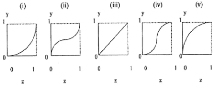
Fig. 7. Graphical expression for the five OPC models.
lots of good and lots of bad samples but few intermediate ones, and v) lots of bad samples. A graphical expression for these five OPC models or types is shown in Fig. 7. To accommodate the above five OPC types and differentiate the curves within one type by using the smallest number of parameters, the inverse mapping of the incomplete Beta function, parameterized by a pair of numbers and , is employed. More precisely, the standardized OPC is determined by a two-parameter smooth
curve ,
where is the Incomplete Beta function of the two parameters . In general, corresponds to the OPC of type (i); corresponds to the OPC of type (ii); corresponds to the OPC of type (iii); corresponds to the OPC of type (iv);
corresponds to the OPC of type (v).
II. Determination of the Size of Selected Subset (SS) for Our Problem [10]
In our problem, the desired number of alignments between SS and , is 1. The corresponding smallest number of alignments between SS and , to achieve the above de-sired alignment is also 1 [13] as indicated in Section I.A. Thus,
we can determine the value by the
formula given in [10], in which we take
is of worst case that is type (v) OPC, and a uniform large noise distribution for the noise char-acteristics . The value of for our problem we obtained from the above formula is 50. It should be noted that the value s we obtained based on the above setup is conservative due to the selection of and .
APPENDIX B
To estimate the value of indicated in Section III.C, we em-ploy the technique of alignment probability [10] as summarized in Appendix A. In the current problem, we apply the following similarities of the terminologies described in Appendix A. We first denote the SS obtained in ii) of the three-stage approach presented in Section III.B as , then treating this as the set in OO theory, that is, we set . Thus, the top
ranked sample in ordered based
on the objective values of will be considered as . In the first phase of our two-phase strategy presented in Section III.C, we use a good approximate model to deter-mine the estimated good enough subset, that is the SS. Now we should determine the size of the SS to ensure that
with very high probability based on the technique of alignment
probability [10]. Since the size of here is only around 50, which is far too small to apply the formula provided in [10] as summarized in Appendix A, we have to perform a Monte Carlo study followed from the guidelines given in [10] to estimate the value (i.e., the size of SS, as described below).
We first place the samples in by
equally spacing them in the normalized ordered interval [0, 1]. We studied a total of 49 OPCs distributed uniformly among the five broadly generic types formed from the
fol-lowing parameters and
, the meaning of the two parameters and are described in Remark 2 of Appendix A. We employ a moderate noise with uniform noise density , because our quadratic approximation for the given in (7) is in fact a good approximate model from the viewpoint of an OPF problem researcher. As a matter of fact, the range of the noise considered above equals the range of OPC, which can result in (with nonzero probability) swapping the rank of some good enough samples with the worst samples. In all of our Monte-Carlo calculations, we simulate 10 000 realizations of noisy OPCs. For the alignment probability equals 0.99, we found that . In other words, . This implies that after solving the quadratic approximate problems shown in
(7), we need only solve exact .
APPENDIX C
We call a sample feasible if the in (3) for the given has a feasible solution; otherwise, we call this infeasible. In addition, we consider the optimal objective value of an infeasible sample as [3]. Obviously, to obtain the top ranked sample of SS ordered by the objective value of , we need to solve the for all samples in SS. However, the samples in SS chosen based on the model (6) do not guarantee to be feasible. Subsequently, we have to answer the question that what if all s samples in SS are infeasible and does one need to search for a feasible solution from ? As a matter of fact, if all s samples of SS are infeasible, then we can be resonably sure (i.e., with probability more than 0.95) the probability that there are feasible samples among the is very low as concluded by the method of point estimation of the opinion poll in statistics ([20], Chap. 3 and [22]). This is briefly illustrated below. Suppose the target population of interest consists of N persons and M of them favor a certain proposition. What we should like to know is the proportion . We consider the opinion poll as a binomial experiment and treat the sample that favors the proposition as a “success.” Then the true success probability p can be estimated by , where denotes the limited number of trials, and denotes the observed number of successes. Now a question is how good is the estimate? Let us determine the probability that the estimate does not deviate from the true success probability p by more than some small quantity d. In other words, we want to know
the probability- -that . Substituting
denotes the probability that k lies in the following range . This probability can be evaluated with the help of normal approximation, and if .
Now our feasibility test can be viewed as the above opinion poll experiment such that the feasible sample is considered as a success. Using the following similarities, and , if there are t feasible samples among the , then we can be resonably sure that the probability of picking up a feasible one from the samples is with deviation not more than , which equals 0.1414. Thus, if all
samples of SS are infeasible, then we can be reasonably sure the probability that there are feasible samples in the N is 0 with deviation not more than 0.1414. This addresses the question raised in (iii) of Section III.B. In the above argument, we inher-ently assume that the samples in SS were uniformly selected; however, this is not our case. As a matter of fact, the samples which are more likely to satisfy the constraints
are more probably selected into SS. This is illustrated below. The criteria that we rank the samples to be selected into SS is according to (6). That is the sample with lower value of will be ranked higher. Since (6) can be rewritten in
the following form , where
. Thus, if is more likely to be feasible then it will cause lower value of and will induce lower value of . Consequently, it will be more probably selected into SS.
APPENDIX D
For the sake of simplicity in explaining the dual-type method for solving the quadratic approximate problem (7), we consider the total generation cost as the objective function, and the in-equality constraints consist of the generation limits and voltage security constraints only. The same method can be applied to the cases with the total system losses as the objective function. Cases including the coupling thermal limit in the inequality con-straints can be similarly treated by taking the modification in [12] into account.
Based on the above assumption, is a convex func-tion of only, thus in the sequel, we use the notation as the objective function. Since the cost of an individual generator is a quadratic function of the generation, thus is a constant diagonal matrix. Furthermore, since the generation limit and voltage security are decoupled bus-wise, the inequality
constraints can be
decom-posed into
(8) where B denotes the number of buses in the system; and denote the increment of continuous variables and the in-equality constraint functions associated with bus . Thus, (7) can be written in the following form:
(9) where the constant matrices
, and , the
con-stant vectors and ,
and the dependent vector
, . Clearly, the matrix is
positive definite, and we can assume that is of full rank, because otherwise we can always delete the redundant equality constraints.
I. DPPQN Method
We will employ the DPPQN method proposed in [11], [12], [14] to solve (9). The DPPQN method solves the following dual problem of (9) instead of solving (9) directly:
(10) where the dual function
(11)
and , where
(12)
and if .
The DPPQN method is an iterative method using the fol-lowing iterations:
(13) where is the iteration index, is a positive step-size deter-mined by an Armijo-type rule [11], [12], [14], and the increment
is computed by
(14) where the matrix
(15) is a negative definite matrix, which represents the Hessian of , however, not considering the constraints as will be shown later in (17). The gradient of at can be com-puted by
(16) where is the optimal solution of the optimization problem on the right-hand side (RHS) of (11), [14].
As shown in [11] and [12], the optimal solution for the op-timization problem on the RHS of (11), , can be obtained using a two-phase approach. The first phase is to solve the fol-lowing unconstrained optimization problem analytically:
(17) which is the optimization problem on the RHS of (11) without considering the constraints . Let be the optimal solution of (17), then
(18) The second phase is to project the onto , that is projecting onto , for , and the resulting projection is the optimal solution of the optimization problem on the RHS of (11), .
1) Summary of the DPPQN Method: Starting from a , we can use the two-phase method mentioned above to solve for
, the optimal solution of the optimization problem on the RHS of (11). Once is obtained, we can compute
by (16). Associated with the matrix expressed in (15), we can solve for from (14). We then update by (13) using an Armijo-type step-size and proceed with the next iteration.
II. Computational Efficiency
We see that the matrix in (15) is sparse, because is di-agonal, and the nonzero entries of represent the structure of the connectivity of the power system, which is sparse. Thus, we can obtain at each iteration by solving the sparse linear (14) using sparse matrix technique. However, the most distin-guished point for applying the DPPQN method here is that the matrix is a constant sparse matrix for all samples
in SS. This implies that the LU factorization and the associated
memory management for the nonzero entries for the sparse ma-trix is done once and for all. This, of course, will save tremen-dous computational-time in solving all the dual problems (10).
III. Convergence and Solution
The in (15) is a negative definite matrix, because is pos-itive definite and is of full rank. Thus, obtained from (14) will be an ascent direction of the dual function (11). With the Armijo-type step-size [11], [12], [14], convergence of the DPPQN method had been shown in [11], [12], and [14]. Let de-note the optimal solution of the dual problem (10), and
denotes the optimal solution of the optimization problem on the RHS of (11) when . Since our primal problem (9) is a quadratic programming problem with a strictly convex objective function, by strong duality theorem [3], the is the solution of (9). Furthermore, if the dual function tends to approach during the solution process, we can conclude that is in-feasible for (7) with the objective value .
REFERENCES
[1] A. Bakirtzis, P. Biskas, C. Zoumas, and V. Petridis, “Optimal power flow by enhanced genetic algorithm,” IEEE Trans. Power Syst., vol. 17, pp. 229–236, May 2002.
[2] A. Bakirtzis and A. Meliopoulos, “Incorporation of switching operation in power system corrective control computations,” IEEE Trans. Power
Syst., vol. 2, pp. 669–676, Aug. 1987.
[3] D. P. Bertsekas, Nonlinear Programming. Belmont, MA: Athena Sci-entific, 1995.
[4] R. Burchet, H. Happ, and D. Vierath, “Quadratically convergent op-timal power flow,” IEEE Trans. Power App. Syst., vol. PAS-103, pp. 3267–3275, Nov. 1985.
[5] L. Chen, H. Suzuki, and K. Katou, “Mean field theory for optimal power flow,” IEEE Trans. Power Syst., vol. 12, pp. 1481–1486, Nov. 1997. [6] T. Giras and N. Talukar, “Quasi-Newton method for optimal power
flows,” Int. J. Electric Power Energy Syst., vol. 3, no. 2, pp. 59–64, Apr. 1981.
[7] Y. C. Ho, Soft Optimization for Hard Problem. Cambridge, MA: Har-vard Univ., 1996. Lecture Notes.
[8] Y. C. Ho, C. C. Cassandras, C. H. Chen, and L. Dai, “Ordinal optimiza-tion and simulaoptimiza-tion,” J. Oper. Res. Soc., vol. 21, pp. 490–500, 2000. [9] T. Kulworawanichpong and S. Sujitjorn, “Optimal power flow using tabu
search,” IEEE Power Eng. Rev., pp. 37–40, June 2002.
[10] T. W. E. Lau and Y. C. Ho, “Universal alignment probability and subset selection for ordinal optimization,” J. Optim. Theory Appl., vol. 39, no. 3, June 1997.
[11] C. Lin and S. Lin, “A new dual-type method used in solving optimal power flow problems,” IEEE Trans. Power Syst., vol. 12, pp. 1667–1675, Nov. 1997.
[12] , “Improvements on the dual-type method used in solving optimal power flow problems,” IEEE Trans. Power Syst., vol. 17, pp. 315–323, May 2002.
[13] S. Lin and Y. C. Ho, “Universal alignment probability revisited,” J.
Optim. Theory Appl., pp. 299–407, May 2002.
[14] S. Lin and C. Lin, “A computationally efficient method for nonlinear multicommodity network flow problems,” Networks, pp. 225–244, July 1997.
[15] W. Liu, A. Papalexopoulos, and W. Tinney, “Discrete shunt controls in a Newton optimal power flow,” IEEE Trans. Power Syst., vol. 7, pp. 1509–1520, Nov. 1992.
[16] D. Luenberger, Linear and Nonlinear Programming, 2nd ed. Reading, MA: Addison-Wesley, 1984.
[17] J. T. Ma and L. L. Lai, “Evolutionary programming approach to reactive power planning,” Proc. Inst. Elect. Eng., vol. 143, Apr. 1996. [18] A. Mantawy, Y. Abdel-Magid, and S. Selim, “Unit commitment by tabu
search,” Proc. Inst. Elect. Eng.-Gen. Transm. Dist., vol. 145, no. 1, pp. 56–64, 1998.
[19] A. Monticelli and W. Liu, “Adaptive movement penalty method for the Newton optimal power flow,” IEEE Trans. Power Syst., vol. 7, pp. 334–340, Feb. 1992.
[20] G. E. Noether, Introduction to Statistics—The Nonparametric
Way. New York, NY: Springer-Verlag, 1991.
[21] B. Stott, J. Marinho, and O. Alsac, “Review of linear programming ap-plied to power system rescheduling,” Proc. IEEE Power Ind. Comput.
Applicat. Conf., pp. 142–154, May 1979.
[22] B. Stott and J. Marinho, “Linear programming for power system network security applications,” IEEE Trans. Power App. Syst., vol. PAS-98, pp. 847–848, May/June 1979.
[23] B. Stott, O. Alsac, and A. Monticelli, “Security analysis and optimiza-tion,” Proc. IEEE, vol. 75, pp. 1623–1664, Dec. 1987.
[24] D. Sun, B. Ashley, B. Brewer, A. Hughes, and W. Tinney, “Optimal power flow by Newton approach,” IEEE Trans. Power App. Syst., vol. PAS-103, pp. 2864–2880, Oct. 1984.
[25] D. Sun, T. Hu, G. Lin, C. Lin, and C. Chen, “Experiences with imple-menting optimal power flow for reactive scheduling in the Taiwan power systems,” IEEE Trans. Power Syst., vol. 3, pp. 1193–1200, Aug. 1988. [26] S. Talukdar and T. Giras, “A fast and robust variable metric method for
optimum power flows,” IEEE Trans. Power App. Syst., vol. PAS-101, pp. 415–420, Feb. 1982.
[27] W. Tinney, J. Bright, K. Demaree, and B. Hughes, “Some deficiencies in optimal power flow,” Proc. IEEE PICA Conf., pp. 164–169, May 1987. [28] G. Torres and V. Quintana, “On a nonlinear multiple-centrality-cor-rections interior-point method for optimal power flows,” IEEE Trans.
Power Syst., vol. 16, pp. 222–228, May 2001.
[29] Y. Wu, “Fuzzy second correction on complementary condition for op-timal power flows,” IEEE Trans. Power Syst., vol. 16, pp. 360–366, Aug. 2001.
[30] Y. Wu, A. Debs, and R. Marsten, “A direct nonlinear predictor-corrector primal-dual interior point algorithm for optimal power flows,” IEEE
Trans. Power Syst., vol. 9, pp. 876–883, May 1994.
Shin-Yeu Lin is currently a Professor in the Department of Electric and Control Engineering at National Chiao Tung University, Hsinchu, Taiwan, R.O.C. His research interests include optimal power flow, ordinal optimization theory, and applications.
Yu-Chi Ho received the S.B. and S.M. degrees in electrical engineering from the Massachusetts Institute of Technology, Cambridge, and the Ph.D. degree in applied mathematics from Harvard University, Cambridge, MA.
Since 1969, he has been Gordon McKay Professor of Engineering and Ap-plied Mathematics at Harvard University. In 1988, he was appointed to the T. Jefferson Coolidge Chair in Applied Mathematics and Gordon McKay Professor of Systems Engineering at Harvard and as Visiting Professor to the Cockrell Family Regent’s Chair in Engineering at the University of Texas, Austin. His research interests include differential games, information structure, multiperson decision analysis, to incentive control, and since 1983, exclusively in discrete event dynamic systems, ordinal optimization, perturbation analysis, and manu-facturing automation.
Ch’i-Hsin Lin is currently an Associate Professor in Electronics Engineering Department at the Kao Yuan Institute of Technology, Kaoshiung Taiwan, R.O.C. His research interests include large scale power systems and ordinal optimiza-tion theory and applicaoptimiza-tions.