LTE隨機存取訊號於可能具有宏大都卜勒位移之多徑通道中之檢測

國 立 交 通 大 學

電子工程學系 電子研究所碩士班

碩 士 論 文

LTE

隨機存取訊號於可能具有宏大都卜勒位移之

多徑通道中之檢測

Detection of LTE Random Access Signals in Multipath

Channels with Possibly Large Doppler Shifts

研 究 生： 梁晉源

LTE 隨機存取訊號於可能具有宏大都卜勒位移之

多徑通道中之檢測

Detection of LTE Random Access Signals in Multipath

Channels with Possibly Large Doppler Shifts

研 究 生: 梁晉源

Student: Chin-Yuan Liang

指導教授: 林大衛

Advisor: Dr. David W. Lin

國 立 交 通 大 學

電子工程學系

電子研究所碩士班

碩 士 論 文

A Thesis

Submitted to Department of Electronics Engineering & Institute of

Electronics

College of Electrical and Computer Engineering

National Chiao Tung University

in Partial Fulfillment of the Requirements

for the Degree of Master of Science

in

Electronics Engineering

October 2013

LTE 隨機存取訊號於可能具有宏大都卜勒位移之

多徑通道中之檢測

研究生：梁晉源

指導教授：林大衛 博士

國立交通大學

電子工程學系 電子研究所碩士班

摘要

本篇論文研究了在於LTE-A的環境下隨機存取偵測的系統，在隨機存取偵測 的過程，基地台必須決定是否使用者傳送了隨機存取前置符元(preamble)。 在論文中，我們建立了傳送系統模型，而當中我們考慮了符元時間偏移、載 波偏移、多徑通道。然後我們把問題制定成多重假說試驗和二元假說試驗，基於 多重假說試驗的實行計算複雜度太高，我們著眼於二元假說試驗。我們使用了普 遍化相似度比率檢驗(generalized ratio likelihood testing, GLRT)當成偵測的準據來 解決問題，而當中我們需要去解出符元時間偏移、載波偏移、多徑通道的最大可 能性估計(maximum likelihood estimate, MLE)。在推導中，我們也提出了一個減 低普遍化相似度比率檢驗的計算複雜度的近似。

在模擬中，在不同載波偏移和多徑通道下，我們驗證了我們提出的普遍化相 似度比率檢驗檢測器的效能。對於多徑通道模型，我們考慮了可加性白色高斯雜 訊(additive white Gaussian noise, AWGN)和史丹佛大學暫定(Standford University Interim, SUI)的模型。

Detection of LTE Random Access Signals in

Multipath Channels with Possibly Large Doppler

Shifts

Student: Chin-Yuan Liang

Advisor: Dr. David W. Lin

Department of Electronics Engineering

& Institute of Electronics

National Chiao Tung University

Abstract

The thesis studies the random access detection schemes in LTE-A system. In random access detection procedure, the base station needs to determine whether random access preambles are transmitted by the users.

In this thesis, we first develop transmission system model, in which we consider the symbol timing offset (STO), carrier frequency offset (CFO), and multipath channels. Then we formulate the problem by the multiple hypothesis and binary hypothesis testing. Due to high computational complexity for implementation of multiple hypothesis testing, we focus on the binary hypothesis testing formulation. We use the generalized likelihood testing technique (GLRT) as a detection criterion to solve the problem, in which we need to get the maximum likelihood estimate (MLE) of the STO, CFO, and channel. In the derivation, we also propose an approximation of the GLRT to further reduce the computational complexity.

誌謝

這篇論文可以完成，首先我要特別感謝我的指導教授林大衛老師，在學術 上，林老師的指導常常讓我如醍醐灌醒般的破解研究上的疑難雜症，此外老師 樹立的風格典範也是我學習的目標，如果沒有林老師，我的研究所生涯可真不 知該何去從，是我生命中的貴人。 此外，還要特別感謝馮智豪老師，因為他的督促，使得我專業知識功力大 增，另外，感謝所有Commlab的老師、杭學鳴教授、簡鳳村教授、桑梓賢教 授、王聖智教授，因著您們的指導，讓我獲益良多。還有感謝在交大我修過課 的所有老師，因著您們慷慨的相授，讓我學習到莫大的知識。 還要感謝，翁郁婷學姐、王柏森學長、洪朝雄學長、林鴻志學長、黃盈叡 學長、江清德學長、柯俊言學長、詹曉盈學長還有其他Commlab的所有學長 姐，給予我在研究過程上的指導與建議，還要感謝政憲、基峰、維哲、義文、 士傑、柔綾、以及所有的成員，因著有你們一起走過，讓我充滿了快樂的回 憶。還要特別感謝男鑫，在論文上的事情上受了你不少的幫忙。 要感謝我電資的好友們，跟你們在一起總是充滿了歡樂，讓我有能量去面 對研究所的任何事情，感謝說說銘，時常和你一起念書做研究，給了我很多的 建議與幫助。要感謝的人太多了，無法一一細數，實感抱歉。 最後我要感謝我生命中的主，若不是祢，我還在黑暗的幽谷，感謝祢每天 的陪伴及指引。 在此，將此篇論文獻給所有陪伴我走過這一段歲月、幫助過我的貴人們。 梁晉源 民國一百零二年 於新竹

Contents

1 Introduction 1

2 Introduction to LTE-A Release 10 Uplink Specifications 3

2.1 Channel Bandwidth . . . 4

2.2 Frame Structure . . . 5

2.2.1 Frame Structure Type 1 . . . 6

2.2.2 Frame Structure Type 2 . . . 6

2.3 Slot Structure and Physical Resources . . . 8

2.3.1 Resource grid . . . 9

2.3.2 Resource elements . . . 9

2.3.3 Resource blocks . . . 10

2.4 Zadoff-Chu Sequences . . . 11

3 Physical Random Access Channel (PRACH) 12 3.1 Time and Frequency Structure . . . 12

4 Random Access Signals Detection for LTE-A 28

4.1 System Model . . . 28

4.2 Problem Formulation . . . 32

4.2.1 Multiple hypothesis testing . . . 32

4.2.2 Binary hypothesis testing . . . 33

4.3 Random Access Techniques Based on GLRT . . . 34

4.3.1 Estimation of CFO . . . 36

4.3.2 Estimation of ICFO, timing offset and channel response . . . 37

4.3.3 GLRT . . . 40

4.3.4 Remarks . . . 40

5 Simulation Results 42 5.1 PRACH Minimum Requirement in TS 36.141 . . . 42

5.2 Simulation Conditions . . . 44

5.3 Simulation Results . . . 46

5.3.1 Performance under AWGN channel . . . 47

5.3.2 Performance anaysis against TS 36.141 . . . 55

5.3.3 Performance under SUI channel . . . 60

6 Conclusion and Future Work 78 6.1 Conclusion . . . 78

Appendix

80

A Multiple Hypothesis Testing 80

List of Figures

2.1 Definition of channel bandwidth and transmission bandwidth configuration

for one E-UTRA carrier [2, Figure 5.6-1]. . . 5

2.2 Frame structure type 1 [3, Figure 4.1-1]. . . 6

2.3 Frame structure type 2 (for 5 ms switch-point periodicity) [3, Figure 4.2-1]. . 7

2.4 Uplink resource grid [3, Figure 5.2.1-1]. . . 10

3.1 Random access preamble format [3, Figure 5.7.1-1]. . . 12

4.1 Transmission system structure. . . 29

4.2 PRACH preamble received at the eNB [5, Figure 17.6]. . . 30

4.3 Singular values. . . 38

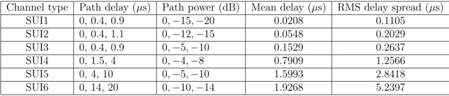
5.1 Pdperformance for solving FCFO and not solving FCFO under AWGN chan-nel for (a) ε = 0 and (b) ε = 0.5. . . . 50

5.2 Histogram ofbεF when ε = 0 for SNR = (a)−40 dB, (b) −30 dB, (c) −20 dB, (d) −10 dB, and (e) 0 dB. . . . 51

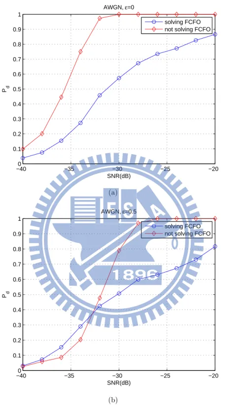
5.3 Pd performance for solving, not solving FCFO, and assuming a perfect esti-mation of FCFO under AWGN channel for (a) ε = 0 and (b) ε = 0.5. . . . . 52

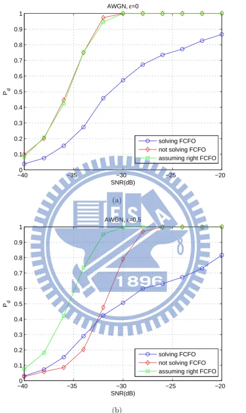
5.4 Pd performance for solving and not solving FCFO under AWGN channel for

different values of ε after adjusting the ICFO search range and FCFO range. 53 5.5 Pd performance for not solving FCFO under AWGN channel for ε = 0 with

different values of L. (b) is a zoom-in plot of (a). . . . 54 5.6 Pd performance for solving and not solving FCFO under AWGN channel for

different values of ε with Pdunder the definition of TS 36.141. (b) is a zoom-in

plot of (a). . . 57 5.7 Pd performance for solving FCFO under ETU70 channel for ε = 0.216 with

Pd under the definition of TS 36.141. (b) is a zoom-in plot of (a). . . 58

5.8 Pd performance for not solving FCFO under ETU70 channel for ε = 0.216

with Pd under the definition of TS 36.141. (b) is a zoom-in plot of (a). . . . 59

5.9 Pdperformance for solving FCFO under SUI1 channel for ε = 0 with different

values of L. . . . 60 5.10 Pdperformance for solving FCFO under SUI2 channel for ε = 0 with different

values of L. . . . 61 5.11 Pdperformance for solving FCFO under SUI3 channel for ε = 0 with different

values of L. . . . 61 5.12 Pdperformance for solving FCFO under SUI4 channel for ε = 0 with different

values of L. . . . 62 5.13 Pdperformance for solving FCFO under SUI5 channel for ε = 0 with different

values of L. . . . 62 5.14 P performance for solving FCFO under SUI6 channel for ε = 0 with different

5.15 Pd performance for not solving FCFO under SUI1 channel for ε = 0 with

different values of L. . . . 64 5.16 Pd performance for not solving FCFO under SUI2 channel for ε = 0 with

different values of L. . . . 64 5.17 Pd performance for not solving FCFO under SUI3 channel for ε = 0 with

different values of L. . . . 65 5.18 Pd performance for not solving FCFO under SUI4 channel for ε = 0 with

different values of L. . . . 65 5.19 Pd performance for not solving FCFO under SUI5 channel for ε = 0 with

different values of L. . . . 66 5.20 Pd performance for not solving FCFO under SUI6 channel for ε = 0 with

different values of L. . . . 66 5.21 Pdperformance for solving FCFO under SUI1 channel with L = 27 for different

values of ε. . . . 67 5.22 Pdperformance for solving FCFO under SUI2 channel with L = 33 for different

values of ε. . . . 68 5.23 Pdperformance for solving FCFO under SUI3 channel with L = 27 for different

values of ε. . . . 68 5.24 Pd performance for solving FCFO under SUI4 channel with L = 122 for

different values of ε. . . . 69 5.25 Pd performance for solving FCFO under SUI5 channel with L = 307 for

5.26 Pd performance for solving FCFO under SUI6 channel with L = 614 for

different values of ε. . . . 70 5.27 Pd performance for solving not FCFO under SUI1 channel with L = 27 for

different values of ε. . . . 71 5.28 Pd performance for solving not FCFO under SUI2 channel with L = 33 for

different values of ε. . . . 72 5.29 Pd performance for solving not FCFO under SUI3 channel with L = 27 for

different values of ε. . . . 72 5.30 Pd performance for solving not FCFO under SUI4 channel with L = 122 for

different values of ε. . . . 73 5.31 Pd performance for solving not FCFO under SUI5 channel with L = 307 for

different values of ε. . . . 73 5.32 Pd performance for solving not FCFO under SUI6 channel with L = 614 for

different values of ε. . . . 74 5.33 Pf a and Pm versus threshold under SUI1 channel with L = 1 and maximum

CIR length for SNR = 10 dB. . . 75 5.34 Pf a and Pm versus threshold under SUI2 channel with L = 1 and maximum

CIR length for SNR = 10 dB. . . 75 5.35 Pf a and Pm versus threshold under SUI3 channel with L = 1 and maximum

CIR length for SNR = 10 dB. . . 76 5.36 Pf a and Pm versus threshold under SUI4 channel with L = 1 and maximum

5.37 Pf a and Pm versus threshold under SUI5 channel with L = 1 and maximum

CIR length for SNR = 10 dB. . . 77 5.38 Pf a and Pm versus threshold under SUI6 channel with L = 1 and maximum

List of Tables

2.1 LTE System Attributes [1, Table 1.1] . . . 4 2.2 Transmission Bandwidth Configuration NRBin E-UTRA Channel Bandwidths

[2, Table 5.6-1] . . . 5 2.3 Uplink-Downlink Configurations [3, Table 4.2-2] . . . 8 2.4 Configuration of Special Subframe (Lengths of DwPTS/GP/UpPTS) [3, Table

4.2-1] . . . 8 2.5 Resource Block Parameters [3, Table 5.2.3-1] . . . 9

3.1 Random access preamble parameters [3, Table 5.7.1-1]. . . 13 3.2 Frame Structure Type 1 Random Access Configuration for Preamble Formats

0–3 [3, Table 5.7.1-2] . . . 14 3.3 Frame Structure Type 2 Random Access Preamble Mapping in Time and

Frequency [3, Table 5.7.1-4] . . . 15 3.4 Frame Structure Type 2 Random Access Configurations for Preamble Formats

0-4 [3, Table 5.7.1-3]. . . 19 3.5 Root Zadoff-Chu Sequence Order for Preamble Formats 0–3 [3, Table 5.7.2-4] 21

3.7 Random Access Preamble Sequence Length [3, Table 5.7.2-1] . . . 24

3.8 NCS for Preamble Generation (Preamble Formats 0–3) [3, Table 5.7.2-2] . . . 25

3.9 NCS for Preamble Generation (Preamble Format 4) [3, Table 5.7.2-3] . . . . 26

3.10 Random Access Baseband Parameters [3, Table 5.7.3-1] . . . 27

5.1 PRACH Detection Test Requirements for Normal Mode [9, Table 8.4.1.5-1] . 43 5.2 PRACH Detection Test Requirements for High Speed Mode [9, Table 8.4.1.5-2] 43 5.3 SNR Correction Factor for PRACH [11, Table 21] . . . 44

5.4 System Parameters for LTE-A Random Access . . . 44

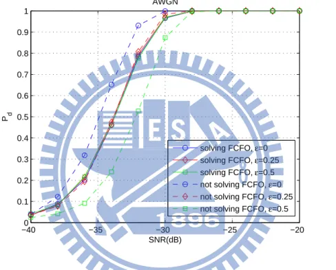
5.5 Mean Delay and RMS Delay Spread of Each SUI Channel Model . . . 45

Chapter 1

Introduction

Single-carrier frequency-division multiple access (SC-FDMA) is the chosen multiple access scheme for the uplink in the 3rd Generation Partnership Project (3GPP) Long Term Evo-lution (LTE), one of the latest standards for cellular mobile communication [1]. The LTE standard is constantly evolving, of which a more recent addition is LTE Advanced (LTE-A), a standard designed to increase the capacity and speed of mobile telephone networks and compliant with IMT-Advanced requirement. LTE Advanced is backwards compatible with LTE and uses the same frequency bands, while LTE is not backwards compatible with the earlier 3G systems. LTE is first introduced in 3GPP release 8. Much of 3GPP release 8 focuses on adopting expected 4G mobile communication technologies, including an all-IP flat networking architecture.

Random access (RA) is generally performed when the user equipment (UE) turns on from sleep mode, performs handoff from one cell to another or when it loses uplink timing syn-chronization. At the time of random access, it is assumed that the UE is time-synchronized with the eNB (the LTE term for base station) on the downlink. Therefore, when a UE turns on from sleep mode, it first needs to acquire downlink timing synchronization. After

transmitting RA preamble. The random access process allows the eNB to estimate and, if needed, adjust the UE uplink transmission timing to within a fraction of the cyclic prefix. After the uplink transmission timing of the UE is synchronized, the UE can be scheduled for uplink transmission.

Our study focuses on LTE-A uplink random access signal detection schemes. Based on 3GPP TS.211 release 10 [3], we construct the random access transmission structure and propose a generalized likelihood ratio test (GLRT) detector which considers both a multipath channel model and carrier frequency offset (CFO). The proposed techniques is different from existing receiver schemes [1, 6]. We will discuss the benefits of assuming a multipath channel model and taking CFO into consideration in the thesis.

The following is a summary of each chapter.

• In chapter 2, we introduce the uplink specifications in the LTE release 10 uplink

stan-dard based on [1, 2, 3, 4].

• In chapter 3, we introduce the random access specification in the LTE release 10 uplink

standard based on [1, 3].

• In chapter 4, we construct the transmission system structure in terms of a mathematical

model based on on [3] and introduce the proposed GLRT receiver scheme.

• In chapter 5, we evaluate our proposed GLRT receiver scheme performance and

com-pare to the method in [5].

Chapter 2

Introduction to LTE-A Release 10

Uplink Specifications

The goal of LTE is to provide a high-data-rate, low-latency and packet-optimized radio access technology supporting flexible bandwidth deployments [1]. In parallel, new network archi-tecture is designed with the goal to support packet-switched traffic with seamless mobility, quality of service and minimal latency.

Some air-interface attributes of the LTE system are summarized in Table 2.1. The system supports flexible bandwidths thanks to SC-FDMA and orthogonal frequency-division multiple access (OFDMA) schemes. In addition to FDD (frequency division duplexing) and TDD (time division duplexing), half duplex FDD is allowed to support low cost UEs. Unlike FDD, in half-duplex FDD operation a UE is not required to transmit and receive at the same time. This avoids the need for a costly duplexer in the UE.

The system is primarily optimized for low speeds up to 15 km/h. However, the system specifications allow mobility support in excess of 350 km/h with some performance degrada-tion. The uplink access based on SC-FDMA promises increased uplink coverage due to low

Table 2.1: LTE System Attributes [1, Table 1.1]

Bandwidth 1.25–20 MHz

Duplexing FDD, TDD, half-duplex FDD

Mobility 350 km/h

Multiple access Downlink OFDMA

Uplink SC-FDMA

MIMO Downlink 2× 2, 4 × 2, 4 × 4

Uplink 1× 2, 1 × 4

Peak data rate in 20 MHz Downlink 173 and 326 Mb/s for 2× 2, 4 × 4 MIMO, respectively

Uplink 86 Mb/s with 1× 2 antenna configuration

Modulation QPSK, 16-QAM and 64-QAM

Channel coding Turbo code

Other techniques

Channel sensitive scheduling, link adaptation, power control, ICIC and hybrid ARQ

MHz bandwidth and higher-order MIMO have been standardized to meet the IMT-advanced requirements.

In this chapter, we introduce the physical channel structure in the LTE-A specifications, focusing on the pplink (UL) part especially.

2.1

Channel Bandwidth

The contents of this section are mainly taken from [2].

Requirements are specified for the channel bandwidths as listed in Table 2.2. Figure 2.1 shows the relation between the channel bandwidth (BWChannel) and the transmission

band-width configuration (NRB). The channel edges are defined as the lowest and highest

Table 2.2: Transmission Bandwidth Configuration NRB in E-UTRA Channel Bandwidths [2, Table 5.6-1] Channel bandwidth BWChannel (MHz) 1.4 3 5 10 15 20 Transmission bandwidth configuration NRB 6 15 25 50 75 100

Figure 2.1: Definition of channel bandwidth and transmission bandwidth configuration for one E-UTRA carrier [2, Figure 5.6-1].

2.2

Frame Structure

The contents of this section are mainly taken from [3].

Throughout the specifications, the size of various fields in the time domain is usually expressed in number of time units Ts = 1/(15000× 2048) seconds.

Downlink and uplink transmissions are organized into radio frames with Tf = 307200×

Ts = 10 ms duration. Two radio frame structures are supported:

Figure 2.2: Frame structure type 1 [3, Figure 4.1-1].

in addition to the primary cell. Unless otherwise noted, the description in the specifications applies to each of the up to five serving cells. In case of multi-cell aggregation, the UE may assume the same frame structure is used in all the serving cells.

2.2.1

Frame Structure Type 1

Frame structure type 1 is shown in Figure 2.2. It is applicable to both full duplex and half duplex FDD. Each radio frame is Tf = 307200× Ts = 10 ms long and consists of 20 slots of

length Tslot = 15360× Ts = 0.5 ms, numbered from 0 to 19. A subframe is defined as two

consecutive slots where subframe i consists of slots 2i and 2i + 1.

For FDD, 10 subframes are available for downlink transmission and 10 subframes are available for uplink transmissions in each 10 ms interval. Uplink and downlink transmissions are separated in the frequency domain. In half-duplex FDD operation, the UE cannot transmit and receive at the same time while there are no such restrictions in full-duplex FDD.

2.2.2

Frame Structure Type 2

Frame structure type 2 is shown in Figure 2.3. It is applicable to TDD. Each radio frame of length Tf = 307200× Ts = 10 ms consists of two half-frames of length 153600× Ts = 5

Figure 2.3: Frame structure type 2 (for 5 ms switch-point periodicity) [3, Figure 4.2-1].

supported uplink-downlink configurations are listed in Table 2.3 where, for each subframe in a radio frame,“D” denotes the subframe is reserved for downlink transmissions,“U” denotes the subframe is reserved for uplink transmissions and “S” denotes a special subframe with the three fields DwPTS, GP and UpPTS. The lengths of DwPTS and UpPTS are given in Table 2.4 subject to the total length of DwPTS, GP and UpPTS being equal to 30720×Ts= 1

ms. Each subframe i is defined as two slots, 2i and 2i + 1 of length Tslot= 15360× Ts = 0.5

ms in each subframe. Uplink-downlink configurations with both 5 ms and 10 ms downlink-to-uplink point periodicity are supported. In case of 5 ms downlink-downlink-to-uplink switch-point periodicity, the special subframe exists in both half-frames. In case of 10 ms downlink-to-uplink switch-point periodicity, the special subframe exists in the first half-frame only. Subframes 0 and 5 and DwPTS are always reserved for downlink transmission. UpPTS and the subframe immediately following the special subframe are always reserved for uplink transmission. In case multiple cells are aggregated, the UE may assume that the guard period of the special subframe in the different cells have an overlap of at least 1456· Ts.

Table 2.3: Uplink-Downlink Configurations [3, Table 4.2-2]

Uplink-downlink Downlink-to-uplink Subframe number

configuration switch-point periodicity 0 1 2 3 4 5 6 7 8 9

0 5 ms D S U U U D S U U U 1 5 ms D S U U D D S U U D 2 5 ms D S U D D D S U D D 3 10 ms D S U U U D D D D D 4 10 ms D S U U D D D D D D 5 10 ms D S U D D D D D D D 6 5 ms D S U U U D S U U D

Table 2.4: Configuration of Special Subframe (Lengths of DwPTS/GP/UpPTS) [3, Table 4.2-1]

Special subframe Normal cyclic prefix in downlink Extended cyclic prefix in downlink

configuration DwPTS UpPTS DwPTS UpPTS

Normal Extended Normal cyclic Extended cyclic

cyclic prefix cyclic prefix prefix in uplink prefix in uplink in uplink in uplink 0 6592· Ts 6592· Ts 1 19760· Ts 20480· Ts 2 21952· Ts 2192· Ts 2560· Ts 23040· Ts 2192· Ts 2560· Ts 3 24144· Ts 25600· Ts 4 26336· Ts 7680· Ts 5 6592· Ts 20480· Ts 6 19760· Ts 23040· Ts 4384· Ts 5120· Ts 7 21952· Ts 4384· Ts 5120· Ts 12800· Ts 8 24144· Ts - - -9 13168· Ts - -

-2.3

Slot Structure and Physical Resources

Table 2.5: Resource Block Parameters [3, Table 5.2.3-1] Configuration N_scRB N_symbU L

Normal cyclic prefix 12 7

Extended cyclic prefix 12 6

2.3.1

Resource grid

The transmitted signal in each slot is described by one or several resource grids of NU L RBNscRB

subcarriers and N_symbU L SC-FDMA symbols. The resource grid is illustrated in Figure 2.4. The quantity N_{N B}U L depends on the uplink transmission bandwidth configured in the cell and shall fulfill

N_RBmin,U L 6 N_RBU L 6 N_RBmax,U L (2.1) where N_RBmin,U L = 6 and N_RBmax,U L = 110 are the smallest and largest uplink bandwidths, respectively, supported by the current version of the LTE specifications. The set of allowed values for N_RBU L is given in [4]. The number of SC-FDMA symbols in a slot depends on the cyclic prefix length configured by the higher layer parameter UL-CyclicPrefixLength and is given in Table 2.5.

2.3.2

Resource elements

Each element in the resource grid is called a resource element and is uniquely defined by the index pair (k, l) in a slot where k = 0, ..., N_RBU LN_scRB − 1 and l = 0, ..., N_symbU L are the indices in the frequency and time domains, respectively. Resource elements that are not used for transmission of a physical channel or a physical signal in a slot shall be set to zero.

Figure 2.4: Uplink resource grid [3, Figure 5.2.1-1].

2.3.3

Resource blocks

A physical resource block is defined as NU L

symb consecutive SC-FDMA symbols in the time

domain and NRB

sc consecutive subcarriers in the frequency domain, where NsymbU L and NscRB

are given by Table 2.5. A physical resource block in the uplink thus consists of NU L

symb× NscRB

resource elements, corresponding to one slot in the time domain and 180 kHz in the frequency domain.

and resource elements (k, l) in a slot is given by nP RB = ⌊ k NRB sc ⌋ . (2.2)

2.4

Zadoff-Chu Sequences

The content of this section are mainly taken from [1]. Zadoff-Chu (ZC) sequences are used extensively in the LTE system, for example, in primary synchronization signals, uplink ref-erence signal, physical uplink shared channel and random access channel [1]. A ZC sequence of length NZC is defined as xu(m) = { e−j πum2 NZC_{, when NZC is even,} e−j πum(m+1) NZC _{,when NZC is odd,} (2.3)

with m = 0, 1, ..., (NZC−1), where u the sequence index, which is relatively prime with NZC.

For a fixed u, the periodic autocorrelation of a ZC sequence is zero for all time shifts other than zero. For different u values, ZC sequences are not orthogonal, but exhibit low crosscorrelation. If the sequence length NZC is a prime number, then there are (NZC − 1)

different sequences with periodic cross-correlation of 1/√NZC between any two sequences

Chapter 3

Physical Random Access Channel

(PRACH)

3.1

Time and Frequency Structure

The contents of this section are mainly taken from [3].

The physical layer random access preamble, illustrated in Figure 3.1, consists of a cyclic prefix of length TCP and a sequence part of length TSEQ. The parameter values are listed in

Table 3.1 and depend on the frame structure and the random access configuration. Higher layers control the preamble format.

The transmission of a random access preamble, if triggered by the MAC layer, is restricted to certain time and frequency resources. These resources are enumerated in increasing order of the subframe number within the radio frame and the physical resource blocks in the fre-quency domain such that index 0 correspond to the lowest numbered physical resource block

Table 3.1: Random access preamble parameters [3, Table 5.7.1-1].

Preamble format TCP TSEQ

0 3168· Ts 24576· Ts

1 21024· Ts 24576· Ts

2 6240· Ts 2· 24576 · Ts

3 21024· Ts 2· 24576 · Ts

4∗ 448· Ts 4096· Ts

* Frame structure type 2 and special subframe configurations with UpPTS lengths 4384· Ts and 5120· Ts only

and subframe within the radio frame. PRACH resources within the radio frame are indicated by a PRACH resource index, where the indexing is in the order of appearance in Table 3.2 and Table 3.3. For frame structure type 1 with preamble format 0–3, there is at most one random access resource per subframe. Table 3.2 lists the preamble formats according to Table 3.1 and the subframes in which random access preamble transmission is allowed for a given configuration in frame structure type 1. The parameter prach-ConfigurationIndex is given by higher layers. The start of the random access preamble shall be aligned with the start of the corresponding uplink subframe at the UE assuming NT A = 0, where NT A

is defined as timing offset between uplink and downlink radio frames at the UE, expressed in units of Ts. For PRACH configurations 0, 1, 2, 15, 16, 17, 18, 31, 32, 33, 34, 47, 48, 49,

50 and 63 the UE may for handover purposes assume an absolute value of the relative time difference between radio frame i in the current cell and the target cell of less than 153600·Ts.

The first physical resource block nRA_{P RB} allocated to the PRACH opportunity considered for preamble formats 0, 1, 2 and 3 is defined as nRA_{P RB} = nRA_{P RBof f set}, where the parameter

prach-FrequencyOffset nRA

P RBof f set, is expressed as a physical resource block number configured by

higher layers and fulfilling 0≤ nRA

Table 3.2: Frame Structure Type 1 Random Access Configuration for Preamble Formats 0–3 [3, Table 5.7.1-2]

PRACH Preamble System Subframe PRACH Preamble System Subframe

configuration format frame number configuration format frame number

index number index number

0 0 Even 1 32 2 Even 1 1 0 Even 4 33 2 Even 4 2 0 Even 7 34 2 Even 7 3 0 Any 1 35 2 Any 1 4 0 Any 4 36 2 Any 4 5 0 Any 7 37 2 Any 7 6 0 Any 1, 6 38 2 Any 1, 6 7 0 Any 2, 7 39 2 Any 2, 7 8 0 Any 3, 8 40 2 Any 3, 8 9 0 Any 1, 4, 7 41 2 Any 1, 4, 7 10 0 Any 2, 5, 8 42 2 Any 2, 5, 8 11 0 Any 3, 6, 9 43 2 Any 3, 6, 9 12 0 Any 0, 2, 4, 6, 8 44 2 Any 0, 2, 4, 6, 8 13 0 Any 1, 3, 5, 7, 9 45 2 Any 1, 3, 5, 7, 9 14 0 Any 0, 1, 2, 3, 4,

5, 6, 7, 8, 9 46 N/A N/A N/A

15 0 Even 9 47 2 Even 9 16 1 Even 1 48 3 Even 1 17 1 Even 4 49 3 Even 4 18 1 Even 7 50 3 Even 7 19 1 Any 1 51 3 Any 1 20 1 Any 4 52 3 Any 4 21 1 Any 7 53 3 Any 7 22 1 Any 1, 6 54 3 Any 1, 6 23 1 Any 2 ,7 55 3 Any 2 ,7 24 1 Any 3, 8 56 3 Any 3, 8 25 1 Any 1, 4, 7 57 3 Any 1, 4, 7 26 1 Any 2, 5, 8 58 3 Any 2, 5, 8 27 1 Any 3, 6, 9 59 3 Any 3, 6, 9

28 1 Any 0, 2, 4, 6, 8 60 N/A N/A N/A

29 1 Any 1, 3, 5, 7, 9 61 N/A N/A N/A

30 N/A N/A N/A 62 N/A N/A N/A

Table 3.3: Frame Structure Type 2 Random Access Preamble Mapping in Time and Fre-quency [3, Table 5.7.1-4]

PRACH UL/DL configuration (See Table 2.3)

configuration Index 0 1 2 3 4 5 6 (See Table 3.4) 0 (0,1,0,2) (0,1,0,1) (0,1,0,0) (0,1,0,2) (0,1,0,1) (0,1,0,0) (0,1,0,2) 1 (0,2,0,2) (0,2,0,1) (0,2,0,0) (0,2,0,2) (0,2,0,1) (0,2,0,0) (0,2,0,2) 2 (0,1,1,2) (0,1,1,1) (0,1,1,0) (0,1,0,1) (0,1,0,0) N/A (0,1,1,1) 3 (0,0,0,2) (0,0,0,1) (0,0,0,0) (0,0,0,2) (0,0,0,1) (0,0,0,0) (0,0,0,2) 4 (0,0,1,2) (0,0,1,1) (0,0,1,0) (0,0,0,1) (0,0,0,0) N/A (0,0,1,1)

5 (0,0,0,1) (0,0,0,0) N/A (0,0,0,0) N/A N/A (0,0,0,1)

6 (0,0,0,2) (0,0,1,2) (0,0,0,1) (0,0,1,1) (0,0,0,0) (0,0,1,0) (0,0,0,1) (0,0,0,2) (0,0,0,0) (0,0,0,1) (0,0,0,0) (1,0,0,0) (0,0,0,2) (0,0,1,1) 7 (0,0,0,1) (0,0,1,1) (0,0,0,0) (0,0,1,0) N/A (0,0,0,0) (0,0,0,2) N/A N/A (0,0,0,1) (0,0,1,0) 8 (0,0,0,0) (0,0,1,0) N/A N/A (0,0,0,0) (0,0,0,1) N/A N/A (0,0,0,0) (0,0,1,1) 9 (0,0,0,1) (0,0,0,2) (0,0,1,2) (0,0,0,0) (0,0,0,1) (0,0,1,1) (0,0,0,0) (0,0,1,0) (1,0,0,0) (0,0,0,0) (0,0,0,1) (0,0,0,2) (0,0,0,0) (0,0,0,1) (1,0,0,1) (0,0,0,0) (1,0,0,0) (2,0,0,0) (0,0,0,1) (0,0,0,2) (0,0,1,1) 10 (0,0,0,0) (0,0,1,0) (0,0,1,1) (0,0,0,0) (0,0,0,1) (0,0,1,1) (0,0,0,0) (0,0,1,0) (1,0,1,0) N/A (0,0,0,0) (0,0,0,1) (1,0,0,0) N/A (0,0,0,0) (0,0,0,2) (0,0,1,0) 11 N/A (0,0,0,0) (0,0,0,1) (0,0,1,0)

N/A N/A N/A N/A

(0,0,0,1) (0,0,1,0) (0,0,1,1) 12 (0,0,0,1) (0,0,0,2) (0,0,1,1) (0,0,1,2) (0,0,0,0) (0,0,0,1) (0,0,1,0) (0,0,1,1) (0,0,0,0) (0,0,1,0) (1,0,0,0) (1,0,1,0) (0,0,0,0) (0,0,0,1) (0,0,0,2) (1,0,0,2) (0,0,0,0) (0,0,0,1) (1,0,0,0) (1,0,0,1) (0,0,0,0) (1,0,0,0) (2,0,0,0) (3,0,0,0) (0,0,0,1) (0,0,0,2) (0,0,1,0) (0,0,1,1) 13 (0,0,0,0) (0,0,0,2) (0,0,1,0) (0,0,1,2) N/A N/A (0,0,0,0) (0,0,0,1) (0,0,0,2) (1,0,0,1) N/A N/A (0,0,0,0) (0,0,0,1) (0,0,0,2) (0,0,1,1) 14 (0,0,0,0) (0,0,0,1) (0,0,1,0) (0,0,1,1) N/A N/A (0,0,0,0) (0,0,0,1) (0,0,0,2) (1,0,0,0) N/A N/A (0,0,0,0) (0,0,0,2) (0,0,1,0) (0,0,1,1)

15 (0,0,0,0) (0,0,0,1) (0,0,0,2) (0,0,1,1) (0,0,1,2) (0,0,0,0) (0,0,0,1) (0,0,1,0) (0,0,1,1) (1,0,0,1) (0,0,0,0) (0,0,1,0) (1,0,0,0) (1,0,1,0) (2,0,0,0) (0,0,0,0) (0,0,0,1) (0,0,0,2) (1,0,0,1) (1,0,0,2) (0,0,0,0) (0,0,0,1) (1,0,0,0) (1,0,0,1) (2,0,0,1) (0,0,0,0) (1,0,0,0) (2,0,0,0) (3,0,0,0) (4,0,0,0) (0,0,0,0) (0,0,0,1) (0,0,0,2) (0,0,1,0) (0,0,1,1) 16 (0,0,0,1) (0,0,0,2) (0,0,1,0) (0,0,1,1) (0,0,1,2) (0,0,0,0) (0,0,0,1) (0,0,1,0) (0,0,1,1) (1,0,1,1) (0,0,0,0) (0,0,1,0) (1,0,0,0) (1,0,1,0) (2,0,1,0) (0,0,0,0) (0,0,0,1) (0,0,0,2) (1,0,0,0) (1,0,0,2) (0,0,0,0) (0,0,0,1) (1,0,0,0) (1,0,0,1) (2,0,0,0) N/A N/A 17 (0,0,0,0) (0,0,0,1) (0,0,0,2) (0,0,1,0) (0,0,1,2) (0,0,0,0) (0,0,0,1) (0,0,1,0) (0,0,1,1) (1,0,0,0) N/A (0,0,0,0) (0,0,0,1) (0,0,0,2) (1,0,0,0) (1,0,0,1)

N/A N/A N/A

18 (0,0,0,0) (0,0,0,1) (0,0,0,2) (0,0,1,0) (0,0,1,1) (0,0,1,2) (0,0,0,0) (0,0,0,1) (0,0,1,0) (0,0,1,1) (1,0,0,1) (1,0,1,1) (0,0,0,0) (0,0,1,0) (1,0,0,0) (1,0,1,0) (2,0,0,0) (2,0,1,0) (0,0,0,0) (0,0,0,1) (0,0,0,2) (1,0,0,0) (1,0,0,1) (1,0,0,2) (0,0,0,0) (0,0,0,1) (1,0,0,0) (1,0,0,1) (2,0,0,0) (2,0,0,1) (0,0,0,0) (1,0,0,0) (2,0,0,0) (3,0,0,0) (4,0,0,0) (5,0,0,0) (0,0,0,0) (0,0,0,1) (0,0,0,2) (0,0,1,0) (0,0,1,1) (1,0,0,2) 19 N/A (0,0,0,0) (0,0,0,1) (0,0,1,0) (0,0,1,1) (1,0,0,0) (1,0,1,0)

N/A N/A N/A N/A

(0,0,0,0) (0,0,0,1) (0,0,0,2) (0,0,1,0) (0,0,1,1) (1,0,1,1) 20 / 30 (0,1,0,1) (0,1,0,0) N/A (0,1,0,1) (0,1,0,0) N/A (0,1,0,1) 21 / 31 (0,2,0,1) (0,2,0,0) N/A (0,2,0,1) (0,2,0,0) N/A (0,2,0,1)

22 / 32 (0,1,1,1) (0,1,1,0) N/A N/A N/A N/A (0,1,1,0)

23 / 33 (0,0,0,1) (0,0,0,0) N/A (0,0,0,1) (0,0,0,0) N/A (0,0,0,1)

24 / 34 (0,0,1,1) (0,0,1,0) N/A N/A N/A N/A (0,0,1,0)

25 / 35 (0,0,0,1) (0,0,1,1) (0,0,0,0) (0,0,1,0) N/A (0,0,0,1) (1,0,0,1) (0,0,0,0) (1,0,0,0) N/A (0,0,0,1) (0,0,1,0) 26 / 36 (0,0,0,1) (0,0,1,1) (1,0,0,1) (0,0,0,0) (0,0,1,0) (1,0,0,0) N/A (0,0,0,1) (1,0,0,1) (2,0,0,1) (0,0,0,0) (1,0,0,0) (2,0,0,0) N/A (0,0,0,1) (0,0,1,0) (1,0,0,1) 27 / 37 (0,0,0,1) (0,0,1,1) (1,0,0,1) (1,0,1,1) (0,0,0,0) (0,0,1,0) (1,0,0,0) (1,0,1,0) N/A (0,0,0,1) (1,0,0,1) (2,0,0,1) (3,0,0,1) (0,0,0,0) (1,0,0,0) (2,0,0,0) (3,0,0,0) N/A (0,0,0,1) (0,0,1,0) (1,0,0,1) (1,0,1,0)

28 / 38 (0,0,0,1) (0,0,1,1) (1,0,0,1) (1,0,1,1) (2,0,0,1) (0,0,0,0) (0,0,1,0) (1,0,0,0) (1,0,1,0) (2,0,0,0) N/A (0,0,0,1) (1,0,0,1) (2,0,0,1) (3,0,0,1) (4,0,0,1) (0,0,0,0) (1,0,0,0) (2,0,0,0) (3,0,0,0) (4,0,0,0) N/A (0,0,0,1) (0,0,1,0) (1,0,0,1) (1,0,1,0) (2,0,0,1) 29 / 39 (0,0,0,1) (0,0,1,1) (1,0,0,1) (1,0,1,1) (2,0,0,1) (2,0,1,1) (0,0,0,0) (0,0,1,0) (1,0,0,0) (1,0,1,0) (2,0,0,0) (2,0,1,0) N/A (0,0,0,1) (1,0,0,1) (2,0,0,1) (3,0,0,1) (4,0,0,1) (5,0,0,1) (0,0,0,0) (1,0,0,0) (2,0,0,0) (3,0,0,0) (4,0,0,0) (5,0,0,0) N/A (0,0,0,1) (0,0,1,0) (1,0,0,1) (1,0,1,0) (2,0,0,1) (2,0,1,0)

40 (0,1,0,0) N/A N/A (0,1,0,0) N/A N/A (0,1,0,0)

41 (0,2,0,0) N/A N/A (0,2,0,0) N/A N/A (0,2,0,0)

42 (0,1,1,0) N/A N/A N/A N/A N/A N/A

43 (0,0,0,0) N/A N/A (0,0,0,0) N/A N/A (0,0,0,0)

44 (0,0,1,0) N/A N/A N/A N/A N/A N/A

45 (0,0,0,0) (0,0,1,0) N/A N/A (0,0,0,0) (1,0,0,0) N/A N/A (0,0,0,0) (1,0,0,0) 46 (0,0,0,0) (0,0,1,0) (1,0,0,0) N/A N/A (0,0,0,0) (1,0,0,0) (2,0,0,0) N/A N/A (0,0,0,0) (1,0,0,0) (2,0,0,0) 47 (0,0,0,0) (0,0,1,0) (1,0,0,0) (1,0,1,0) N/A N/A (0,0,0,0) (1,0,0,0) (2,0,0,0) (3,0,0,0) N/A N/A (0,0,0,0) (1,0,0,0) (2,0,0,0) (3,0,0,0) 48 (0,1,0,*) (0,1,0,*) (0,1,0,*) (0,1,0,*) (0,1,0,*) (0,1,0,*) (0,1,0,*) 49 (0,2,0,*) (0,2,0,*) (0,2,0,*) (0,2,0,*) (0,2,0,*) (0,2,0,*) (0,2,0,*)

50 (0,1,1,*) (0,1,1,*) (0,1,1,*) N/A N/A N/A (0,1,1,*)

51 (0,0,0,*) (0,0,0,*) (0,0,0,*) (0,0,0,*) (0,0,0,*) (0,0,0,*) (0,0,0,*)

52 (0,0,1,*) (0,0,1,*) (0,0,1,*) N/A N/A N/A (0,0,1,*)

53 (0,0,0,*) (0,0,1,*) (0,0,0,*) (0,0,1,*) (0,0,0,*) (0,0,1,*) (0,0,0,*) (1,0,0,*) (0,0,0,*) (1,0,0,*) (0,0,0,*) (1,0,0,*) (0,0,0,*) (0,0,1,*) 54 (0,0,0,*) (0,0,1,*) (1,0,0,*) (0,0,0,*) (0,0,1,*) (1,0,0,*) (0,0,0,*) (0,0,1,*) (1,0,0,*) (0,0,0,*) (1,0,0,*) (2,0,0,*) (0,0,0,*) (1,0,0,*) (2,0,0,*) (0,0,0,*) (1,0,0,*) (2,0,0,*) (0,0,0,*) (0,0,1,*) (1,0,0,*) 55 (0,0,0,*) (0,0,1,*) (1,0,0,*) (0,0,0,*) (0,0,1,*) (1,0,0,*) (0,0,0,*) (0,0,1,*) (1,0,0,*) (0,0,0,*) (1,0,0,*) (2,0,0,*) (0,0,0,*) (1,0,0,*) (2,0,0,*) (0,0,0,*) (1,0,0,*) (2,0,0,*) (0,0,0,*) (0,0,1,*) (1,0,0,*)

56 (0,0,0,*) (0,0,1,*) (1,0,0,*) (1,0,1,*) (2,0,0,*) (0,0,0,*) (0,0,1,*) (1,0,0,*) (1,0,1,*) (2,0,0,*) (0,0,0,*) (0,0,1,*) (1,0,0,*) (1,0,1,*) (2,0,0,*) (0,0,0,*) (1,0,0,*) (2,0,0,*) (3,0,0,*) (4,0,0,*) (0,0,0,*) (1,0,0,*) (2,0,0,*) (3,0,0,*) (4,0,0,*) (0,0,0,*) (1,0,0,*) (2,0,0,*) (3,0,0,*) (4,0,0,*) (0,0,0,*) (0,0,1,*) (1,0,0,*) (1,0,1,*) (2,0,0,*) 57 (0,0,0,*) (0,0,1,*) (1,0,0,*) (1,0,1,*) (2,0,0,*) (2,0,1,*) (0,0,0,*) (0,0,1,*) (1,0,0,*) (1,0,1,*) (2,0,0,*) (2,0,1,*) (0,0,0,*) (0,0,1,*) (1,0,0,*) (1,0,1,*) (2,0,0,*) (2,0,1,*) (0,0,0,*) (1,0,0,*) (2,0,0,*) (3,0,0,*) (4,0,0,*) (5,0,0,*) (0,0,0,*) (1,0,0,*) (2,0,0,*) (3,0,0,*) (4,0,0,*) (5,0,0,*) (0,0,0,*) (1,0,0,*) (2,0,0,*) (3,0,0,*) (4,0,0,*) (5,0,0,*) (0,0,0,*) (0,0,1,*) (1,0,0,*) (1,0,1,*) (2,0,0,*) (2,0,1,*)

58 N/A N/A N/A N/A N/A N/A N/A

59 N/A N/A N/A N/A N/A N/A N/A

60 N/A N/A N/A N/A N/A N/A N/A

61 N/A N/A N/A N/A N/A N/A N/A

62 N/A N/A N/A N/A N/A N/A N/A

63 N/A N/A N/A N/A N/A N/A N/A

For frame structure type 2 with preamble formats 0-4, there might be multiple ran-dom access resources in an UL subframe (or UpPTS for preamble format 4) depending on the UL/DL configuration (see Table 2.3). Table 3.4 lists PRACH configurations allowed for frame structure type 2 where the configuration index corresponds to a certain combination of preamble format, PRACH density value, DRAand version index, rRA. The parameter

prach-ConfigurationIndex is given by higher layers. For frame structure type 2 with PRACH

con-figuration 0, 1, 2, 20, 21, 22, 30, 31, 32, 40, 41, 42, 48, 49, 50, or with PRACH concon-figuration 51, 53, 54, 55, 56, 57 in UL/DL configuration 3, 4, 5, the UE may for handover purposes assume an absolute value of the relative time difference between radio frame i in the current cell and the target cell is less than 153600· Ts.

Table 3.3 lists the mapping to physical resources for the different random access oppor-tunities needed for a certain PRACH density value, DRA. Each quadruple of the format

Table 3.4: Frame Structure Type 2 Random Access Configurations for Preamble Formats 0-4 [3, Table 5.7.1-3]. PRACH configura-tion Index Preamble Format Density Per 10 ms DRA Version rRA PRACH configura-tion Index Preamble Format Density Per 10 ms DRA Version rRA 0 0 0.5 0 32 2 0.5 2 1 0 0.5 1 33 2 1 0 2 0 0.5 2 34 2 1 1 3 0 1 0 35 2 2 0 4 0 1 1 36 2 3 0 5 0 1 2 37 2 4 0 6 0 2 0 38 2 5 0 7 0 2 1 39 2 6 0 8 0 2 2 40 3 0.5 0 9 0 3 0 41 3 0.5 1 10 0 3 1 42 3 0.5 2 11 0 3 2 43 3 1 0 12 0 4 0 44 3 1 1 13 0 4 1 45 3 2 0 14 0 4 2 46 3 3 0 15 0 5 0 47 3 4 0 16 0 5 1 48 4 0.5 0 17 0 5 2 49 4 0.5 1 18 0 6 0 50 4 0.5 2 19 0 6 1 51 4 1 0 20 1 0.5 0 52 4 1 1 21 1 0.5 1 53 4 2 0 22 1 0.5 2 54 4 3 0 23 1 1 0 55 4 4 0 24 1 1 1 56 4 5 0 25 1 2 0 57 4 6 0

26 1 3 0 58 N/A N/A N/A

27 1 4 0 59 N/A N/A N/A

28 1 5 0 60 N/A N/A N/A

29 1 6 0 61 N/A N/A N/A

(fRA, t (0) RA, t (1) RA, t (2)

RA) indicates the location of a specific random access resource, where fRA

is a frequency resource index within the considered time instance, t(0)_RA = 0, 1, 2 indicates whether the resource is reoccurring in all radio frames, in even radio frames, or in odd radio frames, respectively, t(1)_RA = 0, 1 indicates whether the random access resource is located in first half frame or in second half frame, respectively, and where t(2)_RA is the uplink subframe number where the preamble starts, counting from 0 at the first uplink subframe between 2 consecutive downlink-to-uplink switch points, with the exception of preamble format 4 where

t(2)_RA is denoted as (*). The start of the random access preamble formats 0–3 shall be aligned with the start of the corresponding uplink subframe at the UE assuming NT A = 0 and the

random access preamble format 4 shall start 4832· Ts before the end of the UpPTS at the

UE, where the UpPTS is referenced to the UE’s uplink frame timing assuming NT A= 0.

The random access opportunities for each PRACH configuration shall be allocated in time first and then in frequency if and only if time multiplexing is not sufficient to hold all opportunities of a PRACH configuration needed for a certain density value DRA without

overlap in time. For preamble format 0–3, the frequency multiplexing shall be done according to nRA_{P RB} = { nRA P RBof f set+ 6 ⌊_f RA 2 ⌋ , if fRA mod 2 = 0, NU L RB − 6 − nRAP RBof f set− 6 ⌊_f RA 2 ⌋ , otherwise, (3.1)

where N_RBU L is the number of uplink resource blocks, nRA_{P RB} is the first physical resource block allocated to the PRACH opportunity considered and where the parameter

prach-Frequencyoffset, nRA

P RBof f set, is the first physical resource block available for PRACH

ex-pressed as a physical resource block number configured by higher layers and fulfilling 0 ≤

nRA

P RBof f set ≤ NRBU L− 6.

For preamble format 4, the frequency multiplexing shall be done according to

nRA_{P RB} = { 6fRA, if ( (nf mod 2)× (2 − NSP) + t (1)) RA ) mod 2 = 0, NU L RB − 6(fRA+ 1), otherwise, (3.2) where nf is the system frame number and where NSP is the number of DL to UL switch points

within the radio frame. Each random access preamble occupies a bandwidth corresponding to 6 consecutive resource blocks for both frame structures.

3.2

Preamble Sequence Generation

The contents of this section are mainly taken from [3].

The random access preambles are generated from Zadoff-Chu sequences with zero corre-lation zone, from one or several root Zadoff-Chu sequences. The network configures the set of preamble sequences the UE is allowed to use. There are 64 preambles available in each cell. The set of 64 preamble sequences in a cell is found by including first, in the order of increasing cyclic shift, all the available cyclic shifts of a root Zadoff-Chu sequence with the logical index RACH ROOT SEQUENCE, where RACH ROOT SEQUENCE is broadcasted as part of the system information. Additional preamble sequences, in case 64 preambles cannot be generated from a single root Zadoff-Chu sequence, are obtained from the root sequences with consecutive logical indexes until all the 64 sequences are found. The logical root sequence order is cyclic: the logical index 0 is consecutive to 837. The relation between a logical root sequence index and physical root sequence index u is given by Tables 3.5 and 3.6 for preamble formats 0–3 and 4, respectively.

Table 3.5: Root Zadoff-Chu Sequence Order for Preamble Formats 0–3 [3, Table 5.7.2-4] Logical root Physical root sequence number u

sequence number (in increasing order of the corresponding logical sequence number) 0–23 129, 710, 140, 699, 120, 719, 210, 629, 168, 671, 84, 755, 105, 734, 93,

746, 70, 769, 60, 779, 2, 837, 1, 838

24–29 56, 783, 112, 727, 148, 691

30–35 80, 759, 42, 797, 40, 799

76–89 95, 744, 202, 637, 190, 649, 181, 658, 137, 702, 125, 714, 151, 688 90–115 217, 622, 128, 711, 142, 697, 122, 717, 203, 636, 118, 721, 110, 729, 89, 750, 103, 736, 61, 778, 55, 784, 15, 824, 14, 825 116–135 12, 827, 23, 816, 34, 805, 37, 802, 46, 793, 207, 632, 179, 660, 145, 694, 130, 709, 223, 616 136–167 228, 611, 227, 612, 132, 707, 133, 706, 143, 696, 135, 704, 161, 678, 201, 638, 173, 666, 106, 733, 83, 756, 91, 748, 66, 773, 53, 786, 10, 829, 9, 830 168–203 7, 832, 8, 831, 16, 823, 47, 792, 64, 775, 57, 782, 104, 735, 101, 738, 108, 731, 208, 631, 184, 655, 197, 642, 191, 648, 121, 718, 141, 698, 149, 690, 216, 623, 218, 621 204–263 152, 687, 144, 695, 134, 705, 138, 701, 199, 640, 162, 677, 176, 663, 119, 720, 158, 681, 164, 675, 174, 665, 171, 668, 170, 669, 87, 752, 169, 670, 88, 751, 107, 732, 81, 758, 82, 757, 100, 739, 98, 741, 71, 768, 59, 780, 65, 774, 50, 789, 49, 790, 26, 813, 17, 822, 13, 826, 6, 833 264–327 5, 834, 33, 806, 51, 788, 75, 764, 99, 740, 96, 743, 97, 742, 166, 673, 172, 667, 175, 664, 187, 652, 163, 676, 185, 654, 200, 639, 114, 725, 189, 650, 115, 724, 194, 645, 195, 644, 192, 647, 182, 657, 157, 682, 156, 683, 211, 628, 154, 685, 123, 716, 139, 700, 212, 627, 153, 686, 213, 626, 215, 624, 150, 689 328–383 225, 614, 224, 615, 221, 618, 220, 619, 127, 712, 147, 692, 124, 715, 193, 646, 205, 634, 206, 633, 116, 723, 160, 679, 186, 653, 167, 672, 79, 760, 85, 754, 77, 762, 92, 747, 58, 781, 62, 777, 69, 770, 54, 785, 36, 803, 32, 807, 25, 814, 18, 821, 11, 828, 4, 835 384–455 3, 836, 19, 820, 22, 817, 41, 798, 38, 801, 44, 795, 52, 787, 45, 794, 63, 776, 67, 772, 72, 767, 76, 763, 94, 745, 102, 737, 90, 749, 109, 730, 165, 674, 111, 728, 209, 630, 204, 635, 117, 722, 188, 651, 159, 680, 198, 641, 113, 726, 183, 656, 180, 659, 177, 662, 196, 643, 155, 684, 214, 625, 126, 713, 131, 708, 219, 620, 222, 617, 226, 613 456–513 230, 609, 232, 607, 262, 577, 252, 587, 418, 421, 416, 423, 413, 426, 411, 428, 376, 463, 395, 444, 283, 556, 285, 554, 379, 460, 390, 449, 363, 476, 384, 455, 388, 451, 386, 453, 361, 478, 387, 452, 360, 479, 310, 529, 354, 485, 328, 511, 315, 524, 337, 502, 349, 490, 335, 504, 324, 515 514–561 323, 516, 320, 519, 334, 505, 359, 480, 295, 544, 385, 454, 292, 547, 291, 548, 381, 458, 399, 440, 380, 459, 397, 442, 369, 470, 377, 462, 410, 429, 407, 432, 281, 558, 414, 425, 247, 592, 277, 562, 271, 568, 272, 567, 264, 575, 259, 580 562–629 237, 602, 239, 600, 244, 595, 243, 596, 275, 564, 278, 561, 250, 589, 246, 593, 417, 422, 248, 591, 394, 445, 393, 446, 370, 469, 365, 474, 300, 539, 299, 540, 364, 475, 362, 477, 298, 541, 312, 527, 313, 526, 314, 525, 353, 486, 352, 487, 343, 496, 327, 512, 350, 489, 326, 513, 319, 520, 332, 507, 333, 506, 348, 491, 347, 492, 322, 517

630–659 330, 509, 338, 501, 341, 498, 340, 499, 342, 497, 301, 538, 366, 473, 401, 438, 371, 468, 408, 431, 375, 464, 249, 590, 269, 570, 238, 601, 234, 605 660–707 257, 582, 273, 566, 255, 584, 254, 585, 245, 594, 251, 588, 412, 427, 372, 467, 282, 557, 403, 436, 396, 443, 392, 447, 391, 448, 382, 457, 389, 450, 294, 545, 297, 542, 311, 528, 344, 495, 345, 494, 318, 521, 331, 508, 325, 514, 321, 518 708–729 346, 493, 339, 500, 351, 488, 306, 533, 289, 550, 400, 439, 378, 461, 374, 465, 415, 424, 270, 569, 241, 598 730–751 231, 608, 260, 579, 268, 571, 276, 563, 409, 430, 398, 441, 290, 549, 304, 535, 308, 531, 358, 481, 316, 523 752–765 293, 546, 288, 551, 284, 555, 368, 471, 253, 586, 256, 583, 263, 576 766–777 242, 597, 274, 565, 402, 437, 383, 456, 357, 482, 329, 510 778–789 317, 522, 307, 532, 286, 553, 287, 552, 266, 573, 261, 578 790–795 236, 603, 303, 536, 356, 483 796–803 355, 484, 405, 434, 404, 435, 406, 433 804–809 235, 604, 267, 572, 302, 537 810–815 309, 530, 265, 574, 233, 606 816–819 367, 472, 296, 543 820–837 336, 503, 305, 534, 373, 466, 280, 559, 279, 560, 419, 420, 240, 599, 258, 581, 229, 610

Table 3.6: Root Zadoff-Chu Sequence Order for Preamble Format 4 [3, Table 5.7.2-5]

Logical Physical root sequence number u

root (in increasing order of the corresponding logical sequence number) sequence number 0–19 1 138 2 137 3 136 4 135 5 134 6 133 7 132 8 131 9 130 10 129 20–39 11 128 12 127 13 126 14 125 15 124 16 123 17 122 18 121 19 120 20 119 40–59 21 118 22 117 23 116 24 115 25 114 26 113 27 112 28 111 29 110 30 109 60–79 31 108 32 107 33 106 34 105 35 104 36 103 37 102 38 101 39 100 40 99 80–99 41 98 42 97 43 96 44 95 45 94 46 93 47 92 48 91 49 90 50 89 100–119 51 88 52 87 53 86 54 85 55 84 56 83 57 82 58 81 59 80 60 79 120–137 61 78 62 77 63 76 64 75 65 74 66 73 67 72 68 71 69 70 - -138–837 N/A

Table 3.7: Random Access Preamble Sequence Length [3, Table 5.7.2-1]

Preamble format NZC

0–3 839

4 139

The uth root Zadoff-Chu sequence is defined by

xu(n) = e−j

πun(n+1))

NZC _{, 0}≤ n ≤ N_ZC − 1, _(3.3)

where the length NZC of the Zadoff-Chu sequence is given by Table 3.7. From the uth

root Zadoff-Chu sequence, random access preambles with zero correlation zones of length

NCS− 1are defined by cyclic shifts according to

xu,v(n) = xu((n + Cv) mod NZC) (3.4)

where the cyclic shift is given by

Cv =    vNCS, v = 0, 1, ...,⌊NZC/NCS⌋ − 1, NCS ̸= 0, 0, NCS = 0, dstart ⌊ v/nRA shif t ⌋ +(vmodnRA shif t )

NCS, v = 0, 1, ..., nRAshif tnRAgroup+ ¯nRAshif t− 1,

(3.5) where the first two lines in the equation are for unrestricted sets and the last line is for restricted sets, and NCS is given by Tables 3.8 and 3.9 for preamble formats 0–3 and 4,

respectively, where the parameter zeroCorrelationZoneConfig is provided by higher layers. The parameter High-speed-flag provided by higher layers determines if unrestricted set or restricted set shall be used.

The variable du is the cyclic shift corresponding to a Doppler shift of magnitude 1/TSEQ

and is given by du = { p, 0≤ p < NZC/2, NZC − p, otherwise, (3.6) where p is the smallest non-negative integer that fulfils (pu)modNZC = 1. The parameters

Table 3.8: NCS for Preamble Generation (Preamble Formats 0–3) [3, Table 5.7.2-2]

zeroCorrelationZoneConf ig NCS value

Unrestricted set Restricted set

0 0 15 1 13 18 2 15 22 3 18 26 4 22 32 5 26 38 6 32 46 7 38 55 8 46 68 9 59 82 10 76 100 11 93 128 12 119 158 13 167 202 14 279 237 15 419 -given by nRA_{shif t}=⌊du/NCS⌋ , dstart= 2du+ nRAshif tNCS, nRA group =⌊NZC/dstart⌋ , ¯ nRA shif t= max (⌊( NZC − 2du− nRAgroupdstart ) /NCS ⌋ , 0). (3.7)

For NZC/3≤ du ≤ (NZC − NCS)/2, the parameters are given by

nRA_{shif t}=⌊(NCS− 2du)/NCS⌋ , dstart= NZC− 2du+ nRAshif tNCS, , nRA group =⌊du/dstart⌋ , ¯ nRA shif t= min (

max(⌊(du− nRAgroupdstart

) /NCS ⌋ , 0), nRA shif t ) . (3.8)

Table 3.9: NCS for Preamble Generation (Preamble Format 4) [3, Table 5.7.2-3] zeroCorrelationZoneConf ig NCS value 0 2 1 4 2 6 3 8 4 10 5 12 6 15 7 N/A 8 N/A 9 N/A 10 N/A 11 N/A 12 N/A 13 N/A 14 N/A 15 N/A

3.3

Baseband Signal Generation

The contents of this section are mainly taken from [3].

The time-continuous random access signal s(t) is defined by

s(t) = βP RACH N∑ZC−1 k=0 N∑ZC−1 n=0 xu,v(n)· e−j 2πnk NZC · ej2π(k+φ+K(k0+1/2))∆fRA(t−TCP) _(3.9)

where 0 ≤ t < TSEQ+ TCP, βP RACH is an amplitude scaling factor, and k0 = nRAP RBNscRB −

NU L

RBNscRB/2 . The location in the frequency domain is controlled by the parameter nRAP RB as

derived from section 3.1. The factor K = ∆f /∆fRA accounts for the difference in subcarrier

spacing between the random access preamble and uplink data transmission. The variable ∆fRA, the subcarrier spacing for the random access preamble, and the variable φ, a fixed

offset determining the frequency-domain location of the random access preamble within the physical resource blocks, are both given by Table 3.10.

Table 3.10: Random Access Baseband Parameters [3, Table 5.7.3-1]

Preamble format ∆fRA φ

0–3 1250 Hz 7

Chapter 4

Random Access Signals Detection for

LTE-A

In this chapter, first we will introduce the system structure and the problem formulation, and then we will describe the GLRT detector considered in the thesis.

4.1

System Model

The transmission structure is shown in Figure 4.1. Because the discrete Fourier trans-form (DFT) precoding of a ZC sequence converts to another ZC sequence with a different root index [1], unlike the transmission of user signals in SC-FDMA, DFT precoding of the random access preamble is unneeded. Therefore, we adopt a direct mapping scheme where DFT-precoding is removed. Random access transmission uses six consecutive re-source blocks, which equals to 1.08 MHz, and is transmitted over B available bandwidth. That is, the system totally uses N = B/∆fRA subcarriers for transmission. For UE k,

NZC points of Zadoff-Chu sequence with root index uk and cyclic shift Cvk denoted by

xuk,vk , [xuk,vk(0) xuk,vk(1)· · · xuk,vk(NZC − 1)]

T

are directly mapped to the input of the

N –point IDFT where the location in the frequency domain is defined in section 3.3. Let ck

Figure 4.1: Transmission system structure. ck(i) = { xuk,vk(i− ϕ) , ϕ ≤ i ≤ ϕ + NZC − 1, 0, otherwsie, (4.1) where 0≤ i ≤ N −1 and ϕ = φ+_∆f∆f RA ( k0+1₂ )

denotes the starting position in the frequency domain.

A transmitted time-domain RA-preamble without CP sk is IDFT of ck given as

sk , [sk(0) sk(1)· · · sk(N − 1)] T = √1 NF H_c k (4.2)

where F∈ CN×N is the normalized DFT matrix defined as

F, √1 N      ω0·0 N ωN0·1 · · · ω 0·(N−1) N ω1·0 N ωN1·1 · · · ω 1·(N−1) N .. . ... . .. ... ω(N_N −1)·0 ω_N(N−1)·1 · · · ω_N(N−1)·(N−1)      (4.3)

with ωN = e−j2π/N. Inserting CP can be regarded as adding a length of NCP which is indexed

as [sk(−NCP) sk(−NCP + 1)· · · sk(−1)] T

Figure 4.2: PRACH preamble received at the eNB [5, Figure 17.6].

Denote by L the maximum length of CIR and assume L > NCP − 1. Denote the CIR by

hk = [hk(0) hk(1)· · · hk(L− 1)] T

. The UE aligns the start of the random access preamble with the start of the corresponding uplink subframe at the UE assuming a timing advance of zero [5]. Figure 4.2 shows two preambles at the eNodeB received with different timings depending on the propagation delay. Denote θk by the timing offset and θk≥ 0.

Here we formulate the convolution operation in matrix form. So let Sk(θ)∈ CN×N be a

Toeplitz matrix containing the transmitted time-domain signal as

Sk(θk) =      sk(−θk) sk(−θk− 1) · · · sk(−θk− (N − 1)) sk(−θk+ 1) sk(−θk) . .. ... .. . . .. . .. sk(θk− 1) sk(−θk+ (N − 1)) · · · sk(−θk+ 1) sk(−θk)      (4.4)

where sk(i) = 0 for i <−NCP. Let ε be the normalized carrier frequency offset (CFO) with

after removing CP by vector y = [y(0) y(1)· · · y(N − 1)]T as y = K ∑ k=1 (qkΓ(εk)Sk(θk)Bhk+ n) (4.5)

where qk denotes the presence of the RA-preamble as

qk =

{

1, if the RA-preamble is present,

0, if the RA-preamble is not present, (4.6)

Γ(ε) = diag ( 1, ej2πNε, ej 2π Nε·2,· · · , ej 2π Nε·(N−1) ) ∈ CN×N _(4.7)

is the phase rotation matrix induced by CFO, B is a matrix to append zeros to make it a

N vector as B = [ I L×L 0(N−L)×L ] , (4.8) and n = [n(0) n(1)· · · n(L− 1) ]T

is a vector of complex additive white Gaussian noise (AWGN) with zero mean and unknown power σ_n2.

We further assume 0 ≤ θ ≤ NCP−(L − 1). That is, y only contains steady-state response

of the channel to all RA-preambles. As a consequence, we can substitute Sk(θk) in (4.4)

with a circulant matrix

eSk(θ) =      sk(−θ) sk(−θ + (N − 1)) · · · sk(−θ + 1)) sk(−θ + 1) sk(−θ) . .. ... .. . . .. . .. sk(θ + (N − 1)) sk(−θ + (N − 1)) · · · sk(−θ + 1) sk(−θ)      (4.9)

and (4.5) can be rewritten as

y =

K

∑

k=1

qkΓ(εk)eSk(θk)Bhk+ n. (4.10)

where Dk(θk) is a diagonal matrix where diagonal entries are the DFT of the first column

of eSk(θk). Because the first column of eSk(θk) is the cyclic shift of sk by−θ, its DFT can be

expressed as

Dk(θk) = Γ(−θk)diag (cu) . (4.12)

Note that

Dk(θk)HDk(θk) = diagH(cu) ΓH(−θk)Γ(−θk)diag (cu) = diagH(cu) diag (cu) = C (4.13)

where C = diag (0, 0,· · · , 0, 1, 1, · · · , 1, 0, 0, · · · , 0) with the 1s locating at element indices from ϕ to ϕ + NZC − 1 along the diagonal and depends on neither θ nor k. We will use this

fact in subsequent derivation.

4.2

Problem Formulation

4.2.1

Multiple hypothesis testing

Considering that multiple RA-preambles may be sent and received at the same time, we can formulate the problem as a multiple hypothesis testing problem. Each RA preamble has two possibilities—sent or not sent. Therefore, there are totally 2K possible combinations of the condition for the preambles. We need to decide which one is true among the 2K hypotheses. Assuming the noise is AWGN, We can write the multiple hypothesis testing problem using minimum distance criterion as

min qk,εk,θk,hk,∀k y− K ∑ k=1 qkΓ(εk)FHDk(θk) FBhk 2 2 . (4.14)

Once we solve the set {qk} in the last equation, we will know what combination of

RA-preambles are sent. We can rewrite (4.14) as

min qk,εk,θk,hk,∀k y−[q1Γ(ε1)FHD1(θ1) FB · · · qKΓ(εK)FHDK(θK) FB ]    h1 .. . hK    2 2 . (4.15)

Keeping qk, εk, θkfixed, the least square (LS) solution of h , [ h1 h2 · · · hK ]T is given by bh =       q1BHFHDH1 (θ1) FΓH(ε1) .. . qKBHFHDHK(θK) FΓH(εK)   [q1Γ(ε1)FHD1(θ1) FB · · · qKΓ(εK)FHDK(θK) FB ]    †    q1BHFHDH1 (θ1) FΓH(ε1) .. . qKBHFHDHK(θK) FΓH(εK)    y (4.16) where superscript † denotes Moore-Penrose pseudoinverse. A one-shot solution of the prob-lem (See Appendix A) is found to have too high a computation complexity for impprob-lementa- implementa-tion. Therefore, we consider the single-user detection strategy in the next subsecimplementa-tion.

4.2.2

Binary hypothesis testing

In the single-user detection strategy, each RA-preamble is detected individually. That is, we decide which one of the following hypothesis is true: H0, the RA-preamble sk is not present

in the observation y; H1, the RA-preamble sk is present in the observation y. For si with

i ̸= k, because it is not orthogonal to sk, if they are generated from ZC-sequences with

different root indices, there will be multiple-access intereference (MAI), which will aggravate the detection performance. Although the individual detection strategy is suboptimal, it has the advantage of having a simple composite binary testing formulation. For RA-preamble

sk, the problem can be written as

{

H0 : y = n,

H1 : y = Γ(εk)FHDk(θk) FBhk+ n,

(4.17)

where n = [n(0) n(1)· · · n(L − 1)]T is a vector of complex AWGN with zero mean and unknown power σ2 _{= σ}2

4.3

Random Access Techniques Based on GLRT

After we formulate our problem as one of binary hypothesis testing, we employ GLRT to decide whether the preamble is present or not. The GLRT is derived from the binary hypothesis testing assumption. Denote by pi the probability density function (pdf) of y

under the hypothesis Hi for i = 0, 1. Then the GLRT can be expressed as: Decide H1 if

p1 ( y;bεk, bθk, bhk,bσH21 ) p0 ( y;bσ2 H0 ) > λ (4.18) where ( bεk, bθk, bhk )

is the ML estimate of (εk, θk, hk) and bσ2Hi is the ML estimate of σ

2

con-ditioned on Hi for i = 0, 1 and λ is a threshold by adjusting which to a suitable value can

attain a certain false alarm probability pf a or detection probability pd. From (4.17), we can

write our pdf of y under Hi for i = 0, 1 as

p1 ( y; εk, θk, hk, σ2 ) = 1 (2πσ2₎N2 e2σ2−1∥y−Γ(εk)F H_D k(θk)FBhk∥ 2 2 (4.19) and p0 ( y; σ2)= 1 (2πσ2₎N2 e2σ2−1∥y∥ 2 2_{. (4.20)}

For H0, the ML estimate bσ_H2₀ is found by solving maxσ2p₀(y; σ2). Maximizing over σ2, we get bσ2 H0 = ∥y∥2 2 N/2. (4.21)

Substituting back into the pdf, we have

p0 ( y;bσ_H2 0 ) = ( N/2 πe∥y∥2₂ )N/2 . (4.22)

For H1, the ML estimates (

bεk, bθk, bhk,bσH21 )

for which we get max εk,θk,hk,σ2 p1 ( y; εk, θk, hk, σ2 ) = max εk,θk,hk,σ2 1 (2πσ2₎N2 e2σ2−1∥y−Γ(εk)F H_D k(θk)FBhk∥ 2 2 = max εk,θk,hk,σ2 1 (2πσ2₎N2 e2σ2−1∥y−Γ(εk)F H_D k(θk)FBhk∥ 2 2 = max σ2 1 (2πσ2₎N2 e −1 2σ2_εk,θk,hkmin ∥y−Γ(εk)F H_D k(θk)FBhk∥ 2 2 . (4.23)

Maximizing over σ2, we get

bσ2 H1 = min εk,θk,hk y− Γ(εk)FHDk(θk) FBhk 2 2 N/2 . (4.24)

Substituting back into (4.25), we obtain

max εk,θk,hk p1 ( y; εk, θk, hk,bσH21 ) =   N/2 πe min εk,θk,hk ∥y − Γ(εk)FHDk(θk) FBhk∥ 2 2   N/2 . (4.25) Further, min εk,θk,hk y− Γ(εk)FHDk(θk) FBhk 2 2 = min_ε k,θk min εk,θk|hk y− Γ(εk)FHDk(θk) FBhk 2 2. (4.26) The inner minimization can be solved by the LS method whose solution is

bhk= [ BHFHDH_k (θk) FΓH(εk)Γ(εk)FHDk(θk) FB ]_† Γ(εk)FHDk(θk) FBy =[BHFHCFB]†BHFHDH_k (θk) FΓH(εk)y. (4.27) Then, min εk,θk min hk|εk,θk y− Γ(εk)FHDk(θk) FBhk 2 2 = min εk,θk y − Γ(εk)FHDk(θk) FB [ BHFHCFB]†BHFHDH_k (θk) FΓH(εk)y 2 2 . (4.28)

length constraint on hk. That is, we define B′ = IN×N and let h′k be an N× 1 vector whose

entries can be any value to replace Bhk. Using the new definition, (4.27) becomes simplified

to bh′ k = [ FHCF]†FHDH_k (θk) FΓH(εk)y = FHDH_k (θk) FΓH(εk)y. (4.29)

Substituting bh′_k back, we have min εk,θk min hk|εk,θk y− Γ(εk)FHDk(θk) FIhk 2 2 = min εk,θk y− Γ(εk)FHDk(θk) FIFHDHk (θk) FΓH(εk)y 2 2 = min εk,θk y− Γ(εk)FHCFΓH(εk)y 2 2. (4.30)

We find that now the minimization depends on εk only, which allows us to get an

maxi-mum likelihood estimation (MLE) of εkfirst under the condition of no CIR length constraint.

Therefore, we will first get εbk by using this assumption. Then we go back to the original

formulation to solve for the timing offsets and do RA-preamble detection.

4.3.1

Estimation of CFO

The MLE of CFO is found by solving b εk = argmin εk y− Γ(εk)FHCFΓH(εk)y 2 2 = argmax εk yΓ(εk)FHCFΓH(εk)y 2 2. (4.31)

After expanding the matrices in (4.31), we can rewrite it as bεk = argmax εk R {_N−1 ∑ k=0 ψ (k) Ryy(k) ωkεN } (4.32) where R{·} denotes the real part of its argument, ψ (k) is the DFT of the diagonal terms of C and Ryy(k) is the temporal autocorrelation of y(m) given as

Ryy(k) =

min{N−1,N−1−k}_∑

m=max{−k,0}