國立高雄大學應用數學系(研究所)
碩士論文
使用代理曲面的多階無微分最佳化方法
Multiple Stage Approaches
in Surrogate Assisted
Derivative Free Optimization
研究生:曾詩婷撰
指導教授:王偉仲
致
謝
首先要先感謝我的指導教授 王偉仲教授以及陳瑞斌教授和莊曜遠教授。在研究 所兩年悉心的指導,當我遇到問題時,總是不厭其煩的指導我。研究所兩年,不 但讓我多了一項寫程式的技能,也讓我學習該如何獨立 思考問題並且解決問題 。 除了要感謝教授們之外,還要感謝系上每位教授們和系辦小姐們的照顧,不管是 在學業上或是生活上總是給予適時的關心,讓我們覺得好像是在一個大家庭中 。 此外,更要感謝一路上一起走過兩年既 歡樂又辛苦的的 98 級夥伴們。碩一時每 個禮拜三的籃球時間,打麻將打到半夜。碩二時打橋牌……等等,什麼瘋狂的事 情我們都做過了。 最後當然要感謝我的家人們,讓我無憂無慮的唸完兩年,完成我的碩士學位,當 我遇到挫折的時候,總是在背後支持我。再次感謝所有曾經幫助過我的人,真的 很謝謝你們。 曾詩婷撰Multiple Stage Approaches
in Surrogate Assisted
Derivative Free Optimization
by
Shi-Ting Tseng
Advisor
Wei-Chung Wang
Department of Applied Mathematics,
National University of Kaohsiung
Kaohsiung, Taiwan 811, R.O.C.
July 2009
Contents
1. Introduction 1
2. The Multiple Stage Optimization Algorithm 2
2.1 Algorithm 3
2.2 The Details of Algorithm
2.2.1 Generate Grid and Choose Initial Experime ntal
Points 5
2.2.2 Surrogate Construction 5
2.2.3 Local Extreme Search 9
3. Numerical Experiments 11
3.1 Two Dimensional Cas e 11
3.2 High Dimensional Case 21
3.3 Comparison 24
4. Conclusion 26
Reference 32
使用代理曲面的多階無微分最佳化方法
指導教授:王偉仲教授 國立台灣大學大學數學所 學生:曾詩婷 國立高雄大學應用數學所 摘要 在電腦模擬實驗過程中,最佳化問題的反應函數通常假定是未知的。因此,找到最 佳解是很困難的。數種區域最佳化方法已經被提議而沒有使用反應函數的微分資訊 。然 而,這些區域最佳化方法只能找到 單一極值,因此如何找到多重極值是一個很重要的議 題。在這篇論文裡,我們的目標是根據更新過代理曲面找到有效的起始點。首先,在每 一個階段先構造一個代理曲面來估計真實且未知的反應曲面 ,然後根據代理曲面,用一 個機制篩選有效的起始點來結合區域最佳化方法。幾個數值實驗顯示我們的方法是有效 的。 關鍵字:代理曲面、多重、最佳化、無微分Multiple Stage Approaches
in Surrogate Assisted
Derivative Free Optimization
Advisor: Professor Wei-Chung Wang Institute of Mathematics National Taiwan University
Student: Shi-Ting Tseng Institute of Applied Mathematics National University of Kaohsiung
ABSTRACT
The paper functions for optimization problems in the computer experiments are usually to be unknown. Hence it is difficult to find optimal points. Several local optimization methods have been proposed without using derivative information of the resp onse function. However, these local methods can only be used to identify one local extreme; hence how to find multiple local extremes is an important issue. In this thesis, our goal is to get the efficient starting points from the improved surrogate surface for local optimization method. Here we construct the surrogate surface in each stage to a pproximate the true but unknown response surface, and then base on this surrogate surface, the starting points are selected by a screening procedure for local optimizers. Numerical experimental results are showed that our method performs well.
1
Introduction
This article considers computer optimization problems, which can be formed as follows:
min y = f (x),
subject to x = (x1, x2, . . . , xn),
where f : Rn → R is the response function, and the experimental region is in Rn. The
response value y is in R. This type of optimization problem has the following three char-acteristics: (I) The response function is unknown or complicated. (II) The computational costs of simulating the function value is too high. (III) The differentiation of function is hard to gain.
In the past few years, researchers have proposed many methods to solve optimization problems. These methods can be divided into ’Local Search Methods’ and ’Global Search Methods’.The Response Surface Method (RSM) is a popular local search method. RSM uses the surrogate model to approximate the true surface. Pattern Search is a different kind of local search method, which does not use surrogate surface. The main concept of Pattern Search is exploring along a pre-specified direction in the experimental domain. Davidon [2] proposed a simple pattern search method, which is the coordinate search. Hook and Jeeve proposed a general notion of a direct search method in [7]. The General-ized Pattern Search (GPS) for derivative-free unconstrained optimization was introduced in [15]. Dennis and Torczon were proposed the parallel pattern search methods in [3], while Kolda and Torczon proposed the Asynchronous Parallel Pattern Search (APPS) method in [8]. Another popular optimization method is the Design and Analysis of Computer Experiment (DACE) method [13]. The DACE method is a stochastic normal process that models the deterministic responses. The space filling designs are employed to sam-ple from the experimental region and the surrogate approximation is comsam-pleted by the kringing method. Multiple-Level Single Linkage (MLSL) was proposed in [12]. MLSL is a multistart method, which runs the local optimization algorithm from m ultiple starting points. The MLSL method is a stochastic algorithm that obtains starting points for the local search by randomly sampling points within the experimental region. Each itera-tion randomly generates new sample points and uses the critical distance and threshold parameter to choose the starting points for the local search.
A two-stage method was proposed in [17]. This two-stage method combines aspects of ”Global Search Method” and ”Local Search Method.” The global search method is applied to get the surrogate surface to trend to the true surface, and then selects the
efficient starting points from the surrogate surface. Finally, use a local optimization method to find the local extremes by efficient starting points. To trend the surrogate surface to be more similar with the true surface, it must take more experimental points to construct the surrogate surface in the first stage. Besides, not overall local extremes were identified according to the results of two stage method. In Ackley function and MBS function, the average of the identified local extremes are 2.06 and 5.57. Hence, this study applies the two stage method to the proposed multiple stage method. The primary goal of this study is to iteratively improve the surrogate surface in each stage and use new starting points to find multiple extremes. This approach uses fewer experimental points to construct surrogate surface at first, then gradually improved to surrogate surface with the information provided by prior stages. Except that we select the new starting points from the new surrogate surface and use the local search method to find the local extremes with the new starting points in each stage.
2
The Multiple Stage Optimization Algorithm
Researchers have proposed many different methods for solving optimization problems. These methods can be divided into two types: global search methods and local search methods. Global search methods provide a radical new way to glean useful information about the unknown response surface using surrogates. However, these algorithms can cost too much in terms of function evaluations. Pattern Search is a typical Local Search Method method that follows a pre-specified direction to search a region. For both global search methods and local search methods, reducing the cost of the function evaluation is always a problem. Therefore, the proposed algorithm is designed to solve this kind of problem.
Our main opinion is that we reform our surrogate surface in each circulation. A good surrogate surface is unnecessary at first. The surrogate surface is improved step by step to approximate the true surface with the information from the prior several stages. First, we construct a new surrogate to simulate the true surface in each stage. After that, use a new surrogate to find new efficient starting points to explore the local extremes with the local search method. Thus, our algorithm not only provides more accurate information about the true surface, but also reduces the cost of function evaluation and finding multiple extremes.
2.1
Algorithm
In this subsection, we introduce the framework of the Multiple Stage Algorithm. First, form a grid partition on the experiment domain, then construct the surrogate with fewer
experimental points. Set an appropriate distance parameter D. If the distance dxibetween
the point xi and the objective point is greater than D, then we set xi to be the possible
starting point. In the first stage, the objective point is the point with the lowest surrogate value. After that, the objective points are the overall explored local extremes. Then fit
a second-order polynomial model in the small domain Dxi associated to these possible
starting points xi to select the starting points. Use these starting points to search local
extremes. If no new starting points are found, then refine the current grid partition to a denser grid partition. Table 1 shows a simple outline of the Multiple Stage Method.
Table 1: The Outline of Multiple Stage Method
1. Generate a grid partition on the experimental region.
2. Choose initial experimental points.
3. Repeat until stopping criterion for refining grid partition is met.
3.1 Repeat until stopping criterion for exploring multiple local extremes is met.
3.1.1 Repeat until stopping criterion for constructing the surrogate surface is met.
3.1.1.1 Construct the surrogate surface.
3.1.1.2 Choose the subsequence experimental points.
3.1.2 Screen the starting points.
3.1.3 Explore the multiple local extremes.
3.2 Refine the grid partition on the experimental region.
Next, it is necessary to prove that the algorithm can find all the local extremes. Our main target is to prove that all the local extremes will be covered by the small domains of all the possible starting points. Only then can the Local Search method be used to search the local extremes in the small domain. Table 2 lists the assumptions required for this algorithm:
Table 2: Assumptions of Algorithm
A1. The side Si of the small domain Dxi must be equal to or less than the grid size.
A2. The proposed parameter D is a positive real number, and it must be smaller than the grid size.
A3. The sequence {Ej} represents the sub domains of the experimental domain E, that
M S j=1 Ej=E and Ej T Ek = φ, ∀j6=k.
Proposition 1. Let form a grid partition dense enough and it contains finite grid points xi, ∀ i = 1, 2, . . . , n on the experimental domain E, and let {yt} be a sequence of the
overall local extreme points on E. According to A1, A2 and A3, all local extreme points will be covered by the small domains of all possible starting points.
Proof.
Denote dxi as the distance between the grid point xi (i = 1, 2, . . . , n−1) and the objective
point with the lowest surrogate value, and set the objective point as a possible starting
point. Because the grid points are finite and by the assumption A2, then dxi ≥ D, ∀
i = 1, 2, . . . , n − 1, so that all the grid points will be the possible starting points. Denote {xi} as a sequence of the possible starting points. Suppose y ∈ {yt} , but y /∈
n
S
i=1
Dxi,
hence y /∈ Dxi, ∀ i = 1, 2, . . . , n.
Because y ∈ E and the grid partition is dense enough, assumption A3 shows that ∃ Ek∈
M
[
j=1
Ej, 3 y ∈ Ek
Since that Ek is a square domain, ∃ xkm on the corner of Ek, m = 1, 2, 3, 4 .
According to assumption A1,
Ek j 4 [ m=1 Dxkm, then y ∈ 4 [ m=1 Dxkm Due to S4 m=1 Dxkm j n S i=1 Dxi, hence y ∈ n [ Dx .
It conflicts with our supposition, so that for any y ∈ yt, it must be covered by all the sub
domains Dxi of possible starting points {xi}, i = 1, 2, . . . , n, then y ∈
n
S
i=1
Dxi. This
completes our proof. .
We can use these possible starting points to search the multiple local extremes with the local optimization method. To promote computational efficiently, fit a local second-order polynomial model in the neighborhoods associated to these possible starting points to determine whether or not they are local extremes.
2.2
The Detail of Algorithm
2.2.1 Generate Grid and Choose Initial Experimental Points
Since f is assumed be unknown, it is necessary to get some information about the response surface by sampling experimental points from the grids. First, generate a grid
and choose initial experimental points from a grid partition denoted by P containing pi
(i = 1, 2, . . . , n) points along each dimension. As a result, there are N = p1, p2, . . . , pn
grid points. For operational convenience, we transform the grid points to a long
vec-tor with length N. For example, 2-dimensional grid points are labeled as Pi1,i2 (i1 =
1, 2, . . . , n1 ; i2 = 1, 2, . . . , n2). Rearrange the grid points to form a n1n2 - by - 1 vector
: [P1,1, P1,2, . . . , Pn1,n2]T. After generating the grid points, choose the initial experimental
points denoted Pinit from P . This study uses Latin hypercube to select these Pinit. Pinit
is denoted as the set of initial experimental points and Pinit ⊂ P .
2.2.2 Surrogate Construction
Since the response function is unknown, it is necessary to construct the surrogate sur-face. The surrogate surface can be constructed using any method, but this article adopts the Kringing method.
• Kringing
Kringing is used to interpolate the surrogate surface of a random field. It is developed in the field of special statistics and it is a commonly used method for surrogate construction in computer experiments. The surrogate surface can be denoted as :
˜
S = α(x)βT + z(x) (1)
where α(x) is a q × 1 vector of q functions in the regression, and β is a q × 1 vector of regression coefficient. z(x) is a Gaussian stochastic process with mean zero and covariance function of the form :
C(s, t) = σ2C
θ(s, t) , (2)
where σ2 > 0 is the process variance C
θ(s, t) is the correlation function. The function is
the distance between s and t. For example, Gauss correlation is :
Cθ(s, t) = exp(−θ k s − t k2) (3)
Given a design X = {s1, . . . , sp}, let yx = {y(s1), . . . , y(sp)}T be the response vector
and consider the linear predictor :
ˆ
y(x) = kT(x)y
x (4)
of y(x) at a unexplored point x. Obtaining a classical repetitive stance, we can replace
yx with the corresponding random quantity Yx = [Y (s1), . . . , Y (sp)]T. The best linear
unbiased predictor (BLUP) is obtained by choosing the p × 1 vector k(x) to minimize :
MSE[ˆy(x)] = E[(kT(x)Y
x − Y (x))2] (5)
subject to the unbiasedness constraint:
E[kT(x)Yx] = E[Y (x)] (6)
Define R = [α(x1), α(x2), . . . , α(xp))]T for the p × q matrix. The p × p matrix D is
and d(x) is the p × 1 vector of correlation between experimental points and a unexplored point x, i.e.
d(x) = Cθ(xi, x) , 1 ≤ i ≤ p (8)
Then the surrogate surface can be constructed as
˜
S(x) = αT(x) ˆβ + dT(x)D−1(Y
x − R ˆβ) (9)
where ˆβ = (RTD−1R)−1RTD−1Y
x is the least-squares estimate of β.
• Choosing Subsequence Experimental Points
After constructing the current surrogate, it is necessary to to choose the next possible ex-perimental grid points to update the surrogate. This study applies four different methods to choose these experimental points.
Method 1 Merit Function by Torczon and Trosset
Torczon and Trosset [16] introduced a method to select the next possible experimental point. The method is according to based on ” merit function ”, and it’s formed as
M(x) = S(x) − ρd(x) , (10)
where ρ ≥ 0. S(x) is the surrogate value at point x, and d(x) is the distance from x to the nearest preceding sample points d(x) = min k x − xi k2. Torczon and Trosset suggested fixing ρ as 50. The next possible experimental point is selected by minimizing M(x).
Method 2 Alteration of Merit Function
ρ(x) is a fixed value in the above method. Here, ρ(x) is as :
ρ(x) = k S(x) k2 k d(x) k2
The next possible experimental point is selected by minimizing M(x).
Method 3 Alteration 2 of Merit Function
In the original merit function, the surrogate S might vary from point to point. Here, we want to unify its value into the interval [0, 1].
M(x) = ¯S(x) − ρ(x)d(x) , (12) where ¯ S(x) = S(x) − max (S(x)) , ρ(x) = k ¯S(x) k2 k d(x) k2 (13) Then the next possible experimental point is selected as the minimizing of M(x).
Method 4 Two-Points Selection
The two-point selection method selects two different possible experimental points. Be-sides searching the local optimal points, we also need to explore the rest of experimental area. Therefore, the first experimental is to find the current unexplored minimal points on the grid, and the second experimental is to select one grid point from the sparest area.
Thus, the first point x1 chosen is located at P \ Pexp, and its surrogate value is denoted
as S(x), that is
˜
x = min {S(x), ∀ x ∈ P \ Pexp } (14)
To identify the second point, we segment the response surface domain. There are ai
(i = 1, 2, . . . , n) partitions along each of the dimensions. Thus, there are Narea = a1, a2,
. . . , an, disjoint blocks. Count the explored experimental points in each block, randomly
choose one point from the block with the fewest explored experimental points.
This study uses a simple and intuitive criterion to stop constructing the surrogate. The surrogate construction stage is stopped when the computational cost for constructing sur-rogate surface runs out. This approach makes it possible to regulate the computational cost of the experimental points in each stage.
2.2.3 Local Extreme Search • Screen The Starting Points
Next, use the surrogate surface to find the proper starting points to search the local ex-tremes. This study proposes a novel method of looking for the starting points. Table 3 outline the screening processes as follows :
Table 3: Outline of Screening Processes
1. Sort the surrogate values.
2. Select the possible starting points. 3. Identify the starting points.
After finding the multiple extremes efficiently, it is necessary to scatter the starting points uniformly over the experimental region. Sort the surrogate value of all grid points
S(x(1)) < S(x(2)) < · · · < S(x(n)). Set the sorted grid points as C = {x(1), x(2), . . . , x(n)}
and ¯C = {x(1)}. The possible starting points are chosen from C with the following two
criteria: (I) If k x(i)− x k2> D, then ¯C = ¯C
S
{x(i)}, ∀x ∈ ¯C and i = 2, 3, . . . , n. (II) No other point x ∈ O is within a distance D, where O is the set of total local extremes
found so far. Here D is the minimal range of all dimensions to multiply a parameter c1,
where c1 ∈ (0, 1). Eventually, these possible starting points are collected in set E.
Next, it is necessary to identify the starting points from the possible starting points. First, fit a local second-order polynomial model in the neighborhoods A associated to each possible starting point to determine whether or not it is local extreme. The polynomial is built according to the spherical central composite design with one center point and
least-square estimation of the second-order coefficients. Here, the half side lˆx of Aˆx associated
to possible starting points ˆx is lˆx = min{D, {min k ˆx − b k2} × c2/
√
2}, for all b ∈ O ∪ E \ {ˆx}. If the possible starting point is determined as a local extreme, then we denote this possible starting point as a starting point and collect these starting points in set SP . Second, use the set of starting points SP to make a distance comparison with the set of used starting points Uto prevent the current starting points from being too similar to the used starting points to search the repetitive exploring path. Hence, for all x ∈ SP , if ∃ a ∈ U, 3 k x − a k2 ≤ qk, then we delete the starting point x, where
qk= lx×
√
The starting points can be identified following the steps above. . If no starting points are selected, all efficient starting points have been identified and the algorithm stops ex-ploring multiple local extremes..
• Explore The Local Extreme
After choosing the starting points, they can be used to search the multiple local extremes. This subsection introduces introduce a local optimal method to search the local extremes. The Pattern Search method is for solving unconstrained or linear constrained
minimiza-tion. It generates a sequence of {xt} in Rn with nonincreasing response function values.
The response function f is evaluated at the finite points on a mesh and determine the point with the lowest function value as the possession. If the new candidate’s function
value is less than the possession i.e f (xt+1) < f (xt), then xt+1is the new possession. The
current possession solution is said to be a mesh local optimizer that means its function value is less than the neighboring points, until we find another improved point. Any route can be used to choose the mesh point as the candidates. This study uses the APPSPACK 4.0 developed by Gray and Kolda [6], which implements an asynchronous parallel pattern search method.
When searching the local extremes, we also collect the explored possessive points. Af-ter exploring the local extremes, we gather overall explored experimental points including
the initial experimental points Pinit, subsequence experimental points and the explored
possessive points to be the initial experimental points for next stage to construct the surrogate surface.
• Refine Grid Partition
Owing to the response function is unknown, so that we can’t confirm the initial grid partition is good enough or not. Therefore, if without any starting points being selected, we believe that we have explored the overall efficient starting points on the current grid partition, and then we refine current grid partition to a new denser grid partition. The grid size of new grid partition is a half of current grid partition. For example, in
two-dimensional there are N = p1, p2, . . . , pn grid points along each of dimensions on the
current grid partition. If no starting points are found, refine the grid partition. After
re-fining the grid partition, there will be Nref ine = p1, p2, . . . , p2n−1 grid points along each
starting points must be shortened. D = D × k, where 0 < k < 1.In the end, a simple criterion is used to stop the grid partitioning and the refining process. This process stops when the maximal time is meant.
3
Numerical Experiments
This section presents the results of the experiments in this study, and compares them with those of the MLSL method.
3.1
Two Dimensional Cases
This study conducts experiments on five different types of functions, including the Ack-ley Function, Muller Brown Function, Griewank Function, TGP Function, and Schwefel Function. We construct the surrogate surface by DACE and we have four different meth-ods to select the next experimental grid point. In each experiment, the computational cost is 5% of all the grid points in the first stage, and 1% of all the grid points in each
subsequent stage. We define Mi represented method i for choosing the next experimental
point, where i = 1, 2, 3, 4. Before showing the results of the functions, the following sections first introduce each experimental function.
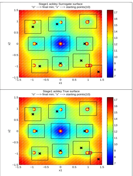
3.1.1 Ackley Function
The first function is called Ackley function, which has been studied previous in [1][14]. Ackley function is formed as:
min f (x, y) = 1 f n − a exp h − b r 1 n(x2+ y2) i − exph 1 n(cos(cx) + cos(cy)) i + a + exp(1) + d o , where a = 20 , b = 0.2 , c = 2π , d = 5.7 , f = 0.8 , n = 2, s.t − 1.5 ≤ x ≤ 1.5 and − 1.5 ≤ y ≤ 1.5
There are 9 local minima at (0, 0), (-0.95, 0), (0.95, 0), (0, -0.95), (0, 0.95), (0.95, 0.95), (0.95, -0.95), (-0.95, 0.95), (-0.95, -0.95). Figure 1 shows the local minima marked by ’x’ on the true surface. First, form a grid partition P containing 625(25 × 25) grid points.
P = n (x, y)| x ∈ {−1.5, −1.5 + 3 24, −1.5 + 6 24, . . . , 1.5}, y ∈ {−1.5, −1.5 + 3 24, −1.5 + 6 24, . . . , 1.5} o
Then choose 25 initial experimental points by Latin hypercube. In Ackley Function, the limit on the computation cost in the first stage is 5% (625× 5% = 31) of all the grid points, after that the limit on the computation cost in each stage is 1% (625× 1% = 6) of
the all the grid points. The parameters for screening starting points are c1 = 0.25, c2 =
0.5 and c3 = 0.5. We summarize the performance of Ackley in Table 4 and the notations
are as follow:
N RT : The number of the stage times.
N GP : The number of the initial experimental points and the subsequence experimental points.
N PSP : The number of the explored possessive points in APPSPACK. N TEP : The total number of experimental points i.e. TEP = GP + PSP N NLP : The number of the local extremes we found.
In Figure 10 to Figure 13, we display the experimental results of M1 to M4. In the
sub-figures, the starting points, the result of APPSPACK, the local extremes and the explored local extremes are marked as ’X’, ’O’, ’+’, ’4’.
3.1.2 MBS Function
The Muller Brown has been studied in [10]. The corresponding optimization problem is defined as : −1.5 −1 −0.5 0 0.5 1 1.5 −1 0 1 7 8 9 10 11 12 13 14 15 16 17 x Ackley True Surface
y 8 9 10 11 12 13 14 15 16 −1 0 1 −1.5 −1 −0.5 0 0.5 1 1.5
Ackley True Surface
x y 8 9 10 11 12 13 14 15 16
Table 4: Performance summary of Ackley Function
Method RT GP PSP TEP NLP M1 3 68 314 382 9 M2 3 68 425 493 9 M3 3 68 394 462 9 M4 5 79 367 446 9 min f (x, y) = 4 X i=1 Aiexp h ai(x − x∗i)2+ bi(x − xi∗)(y − y∗i) + ci(y − yi∗)2 i , where A = (−200, −100, −170, 15), a = (−1, −1, −6.5, 0.7), b = (0, 0, 11, 0.6), c = (−10, −10, −6.5, 0.7), x∗ = (1, 0, −0.5, −1), y∗ = (0, 0.5, 1.5, 1). s.t −1.5 ≤ x ≤ 1 and − 0.5 ≤ y ≤ 2There are 3 local minima at (-0.558, 1.442), (0.623, 0.028) and (-0.05, 0.467). Figure 2 shows the local minima marked by ’x’ on the true surface. We form a grid partition P containing 625(25 × 25) grid points.
P = n (x, y)| x ∈ {−1.5, −1.5 +2.5 24, −1.5 + 5 24, . . . , 1}, y ∈ {−0.5, −0.5 + 2.5 24, −0.5 + 5 24, . . . , 2} o −1.5 −1 −0.5 0 0.5 1 −0.5 0 0.5 1 1.5 2 −200 0 200 400 600 800 1000 1200 1400 1600 1800 x MBS True Surface y −100 −50 0 50 100 150 200 250 300 −1.5 −1 −0.5 0 0.5 1 −0.5 0 0.5 1 1.5 2 MBS True Surface x y −100 −50 0 50 100 150 200 250 300
The number of initial experimental points is 25. In Muller Brown Function, the limit on the computational cost in first stage is 5% (625× 5% = 31) of all the grid points, after that the limit on the computation cost in each stage is 1% (625× 1% = 6) of the all the grid
points. The parameters for screening starting points are c1 = 0.25, c2 = 0.5 and c3 = 0.5.
The performance of Muller Brown is summarized in Table 5:
Table 5: Performance summary of MBS Function
Method RT GP PSP TEP NLP
M1 5 80 354 434 3
M2 4 74 292 366 3
M3 3 68 223 291 3
M4 3 67 235 302 3
In Figure 14 to Figure 17, we display the experimental results of M1 to M4. In the
sub-figures, the starting points, the result of APPSPACK, the local extremes and the explored local extremes are marked as ’X’, ’O’, ’+’, ’4’.
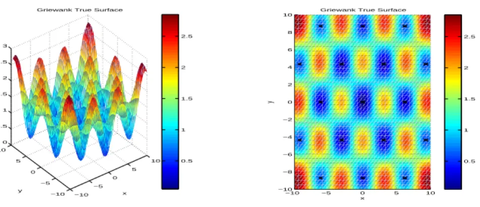
3.1.3 Griewank Function
Now we want to consider the Griewank Function, which has been studied in [11], and the optimization problem is defined as :
min f (x, y) = a + b1x2+ b2y2− d cos(c1x) cos(c2y),
where a = 1; b1, b2 = 1
200; c1 = 1; c2 = √12; d = 1
s.t −10 ≤ x ≤ 10 and − 10 ≤ y ≤ 10
There are 17 local minima at (0, 0),(3.1105, 4.4),(3.1105, -4.4),(-3.1105, 4.4), (-3.1105, -4.4), (6.2209, 0), (-6.2209, 0), (0, 8.7111), (0, -8.7111), (9.3313, 4.4), (9.3313, -4.4), 9.3313, 4.4), 9.3313, -4.4), (6.2209, 8.7111), (6.2209, -8.7111), 6.2209, 8.7111) , (-6.2209, -8.7111). Figure 3 shows the local minima marked by ’x’ on the true surface. We form a grid partition P containing 1600(40 × 40) grid points.
−10 −5 0 5 10 −10 −5 0 5 10 0 0.5 1 1.5 2 2.5 3 x Griewank True Surface
y 0.5 1 1.5 2 2.5 −10 −5 0 5 10 −10 −8 −6 −4 −2 0 2 4 6 8 10
Griewank True Surface
x y 0.5 1 1.5 2 2.5
Figure 3: The true response of Griewank function.
P = n (x, y)| x ∈ {−10, −10 + 20 39, −10 + 40 39, . . . , 10}, y ∈ {−10, −10 + 20 39, −10 + 40 39, . . . , 10} o
We choose 40 initial experimental points by Latin hypercube. In Griewank Function, the limit on the computational cost in first stage is 5% (1600× 5% = 80) of all the grid points, after that the limit on the computation cost in each stage is 1% (1600× 1% = 16)
of the all the grid points. The parameters for screening starting points are c1 = 0.2, c2 =
0.45 and c3 = 0.5. The performance of Griewank is summarized in Table 6:
Table 6: Performance summary of Griewank Function
Method RT GP PSP TEP NLP
M1 3 152 610 762 17
M2 3 152 627 779 17
M3 3 152 643 795 17
M4 5 184 637 821 17
In Figure 18 to Figure 21, we display the experimental results of M1 to M4. In the
sub-figures, the starting points, the result of APPSPACK, the local extremes and the explored local extremes are marked as ’X’, ’O’, ’+’, ’4’.
3.1.4 TGP Function
The next one is TGP function, which has been studied in [9], and the optimization problem is defined as :
min f (x, y) = h
− exp(−(x − 1)2) − exp(a(x + 1)2) + b sin(c(x + 0.1)) i ×
h
exp(−(y − 1)2) + exp(a(y + 1)2) − b sin(c(y + 0.1))i
where a = −0.8, b = 0.05, c = 8. s.t −2 ≤ x ≤ 2 and − 2 ≤ y ≤ 2
There are 16 local minima at (-1.0408, -1.0408), (-1.0408, 1.1366), (1.1366, -1.0408), (-1.0408, 0.6172), (0.6172, -1.0408), (1.1366, 1.1366), (1.1366, 0.6172), (0.6172, 1.1366), (0.6172, 0.6172), (-1.0408, -0.4179), (-0.4179, -1.0408), (-1.0408, 1.1366), (1.1366, -0.4179), (-0.4179, 0.6172), (0.6172, -0.4179), (-0.4179, -0.4179). Figure 4 shows the local minima marked by ’x’ on the true surface. We form a grid partition P containing 1600(40 × 40) grid points. P = n (x, y)| x ∈ {−2, −2 + 4 39, −2 + 8 39, . . . , 2}, y ∈ {−2, −2 + 4 39, −2 + 8 39, . . . , 2} o
We choose 40 initial experimental points by Latin hypercube. In TGP Function, the limit on the computational cost in first stage is 5% (1600× 5% = 80) of all the grid points, after that the limit on the computation cost in each stage is 1% (1600× 1% = 16) of
the all the grid points. The parameters for screening starting points are c1 = 0.15, c2 =
0.4 and c3 = 0.3. The performance of TGP is summarized in Table 7:
In Figure 22 to Figure 25, we display the experimental results of M1 to M4. In the
−2 −1 0 1 2 −2 −1 0 1 2 −1.4 −1.2 −1 −0.8 −0.6 −0.4 −0.2 0 x TGP True Surface y −1.1 −1 −0.9 −0.8 −0.7 −0.6 −0.5 −0.4 −0.3 −0.2 −2 −1 0 1 2 −2 −1.5 −1 −0.5 0 0.5 1 1.5 2 TGP True Surface x y −1.1 −1 −0.9 −0.8 −0.7 −0.6 −0.5 −0.4 −0.3 −0.2
Table 7: Performance summary of TGP Function
Method RT GP PSP TEP NLP M1 6 200 738 938 16 M2 6 200 593 793 16 M3 6 200 880 1080 16 M4 6 184 854 1038 16sub-figures, the starting points, the result of APPSPACK, the local extremes and the explored local extremes are marked as ’X’, ’O’, ’+’, ’4’.
Because of the initial grid partition of the above four functions are good enough, overall local extremes had been explored with the initial grid partition without refining. Next, we show a different case. In this case, the initial grid partition is not good enough, so it needs to refine the grid partition.
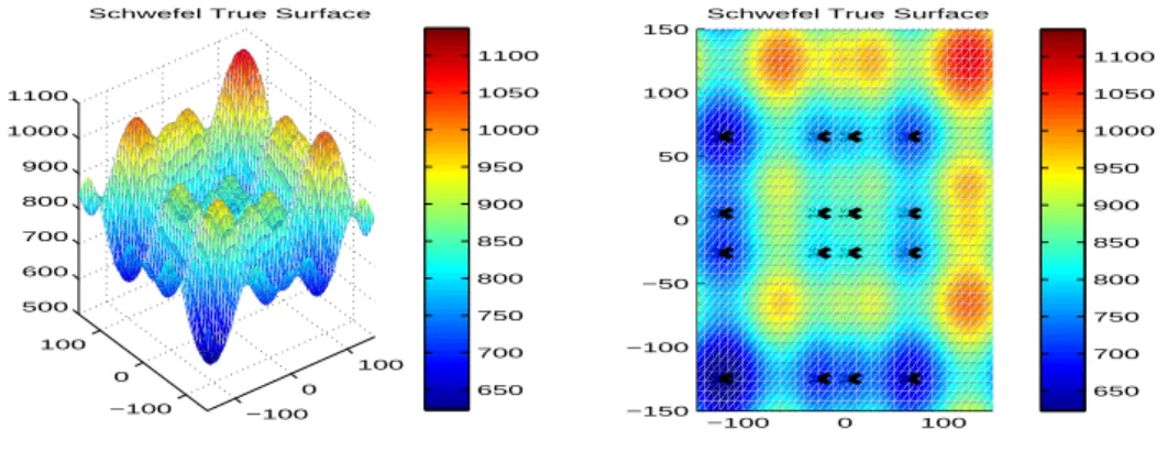
3.1.5 Schwefel Function
The last case is Schwefel Function, which has been studied in [5]. The optimization problem is defined as :
min f (x, y) = 418.9829 × 2 − [ x sin(p|x|) + y sin(p|y|) ]
s.t −150 ≤ x ≤ 150 and − 150 ≤ y ≤ 150
There are 16 local minima at (65.5479, -25.8774), (65.5479, 5.2393), (5.2393, -25.8774), (65.5479, 124.8332), (65.5479, 65.5481), (5.2392, 5.2392), (25.8772, 25.8774), (5.239, -124.8294), (5.2391, 65.5479), (-25.8774, 5.2393), (-124.8291, -25.8774), (-25.8772, --124.8294), (-25.8774, 65.548), (-124.8294, 5.2394), (-124.8291, -124.8294), (-124.8294, 65.5481).
Figure 5 shows the local minima marked by ’x’ on the true surface. The maximal refining
time is 2 times and generate the grid partition P1 containing 36 (6 × 6) grid points.
P1 = n (x, y)| x ∈ {−150, −150 + 300 5 , −150 + 600 5 , . . . , 150}, y ∈ {−150, −150 + 300 5 , −150 + 600 5 , . . . , 150} o
We choose 6 initial experimental points by Latin hypercube. The limit on the com-putational cost in the first stage is 9% of all grid points, after that the limit on the
−100 0 100 −100 0 100 500 600 700 800 900 1000 1100
Schwefel True Surface
650 700 750 800 850 900 950 1000 1050 1100 −100 0 100 −150 −100 −50 0 50 100 150
Schwefel True Surface
650 700 750 800 850 900 950 1000 1050 1100
Figure 5: The true response of Schwefel function.
computational cost in each stage is 5%. The parameters for screening starting points are
c1 = 0.25, c2 = 0.45 and c3 = 0.5. Set the parameter k = 0.7 to shorten D in each stage.
Since there are no more starting points are found in stage2 and stage3, so we refine the
grid partition P1 to P2 containing 121 (11 × 11) grid points for stage3. By the same way,
refine the grid partition P2 to P3 containing 441 (21 × 21) grid points for stage4. The
performance of Schwefel function is summarized in Table 8 and the notation RET is the refining times.
Table 8: Performance summary of Schwefel Function
Method RT RET GP PSP TEP NLP
M1 5 2 60 625 685 16
M2 5 2 60 625 685 16
M3 5 2 60 625 685 16
In Figure 6, we display the experimental results of M1 from stage1 to stage5. In the
sub-figures, the starting points, the result of APPSPACK, the local extremes and the explored local extremes are marked as ’X’, ’O’, ’+’, ’4’.
Figure 6: The true and surrogate surface of Schwefel with M1 −150 −100 −50 0 50 100 150 −150 −100 −50 0 50 100 150
Stage1 (Refine Time = 0) Surrogate surface "o" −−> final min; "x" −−> starting points(18)
x1 x2 650 700 750 800 850 900 950 1000 1050 1100 −150 −100 −50 0 50 100 150 −150 −100 −50 0 50 100 150
Stage1 (Refine Time = 0) True surface "o" −−> final min; "x" −−> starting points(18)
x1 x2 650 700 750 800 850 900 950 1000 1050 1100
−150 −100 −50 0 50 100 150 −150 −100 −50 0 50 100 150 x1
Stage2 ( Refine Time = 0 ) Surrogate surface
x2 650 700 750 800 850 900 950 1000 1050 1100 −150 −100 −50 0 50 100 150 −150 −100 −50 0 50 100 150 x1
Stage3 ( Refine Time = 1) Surrogate surface
x2 650 700 750 800 850 900 950 1000 1050 1100 −150 −100 −50 0 50 100 150 −150 −100 −50 0 50 100 150
Stage4 (Refine Time = 2) Surrogate surface "o" −−> final min; "x" −−> starting points(7)
x1 x2 650 700 750 800 850 900 950 1000 1050 1100 −150 −100 −50 0 50 100 150 −150 −100 −50 0 50 100 150
Stage4 (Refine Time = 2) True surface "o" −−> final min; "x" −−> starting points(7)
x1 x2 650 700 750 800 850 900 950 1000 1050 1100
−150 −100 −50 0 50 100 150 −150 −100 −50 0 50 100 150 x1
Stage5 ( Refine Time = 2) Surrogate surface
x2 650 700 750 800 850 900 950 1000 1050 1100
3.2
High Dimensional Cases
In this section, we consider two cases of three dimension, Ackley Function and Hartman Function. In each experimental function, we set the computational cost as 5% of all grid points in the first stage. After that, the limit on the computational cost in each stage is 1% of all grid points.
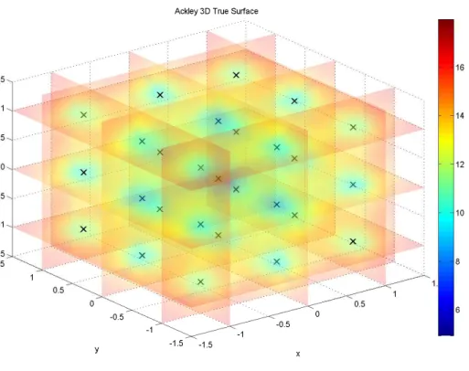
3.2.1 3D Ackley Function
3D Ackley Function has been studied in [1][14]. The function is defined as :
min f (x, y) = 1 f n − a exp h − b r 1 n(x2+ y2+ z2) i − exph 1
n(cos(cx) + cos(cy) + cos(cz))
i + a + exp(1) + d o , where a = 20 , b = 0.2 , c = 2π , d = 5.7 , f = 0.8 , n = 2, s.t − 1.5 ≤ x ≤ 1.5 and − 1.5 ≤ y ≤ 1.5 − 1.5 ≤ z ≤ 1.5
There are 27 local minima, the true response surface and the local minima marked by ’x’ in the true response surface are shown in Figure 7. We form a grid partition P containing 3375(15 × 15 × 15) grid points. P = n(x, y)| x ∈ {−1.5, −1.5 + 3 14, −1.5 + 6 14, . . . , 1.5}, y ∈ {−1.5, −1.5 + 3 14, −1.5 + 6 14, . . . , 1.5}, z ∈ {−1.5, −1.5 + 3 14, −1.5 + 6 14, . . . , 1.5} o
Figure 7: The true response of Ackley 3D function.
We choose 15 initial experimental points by Latin hypercube. In 3D Ackley Function, the limit on the computational cost in the first stage is 5% (3375 × 5% = 168) of all grid points, after that the limit on the computational cost in each stage is 1% (3375 × 1% =
33)of all grid points. The parameters for screening starting points are c1 = 0.25, c2 =
0.5 and c3 = 0.5. The performance of 3D Ackley Function is summarized in Table 9:
Table 9: Performance summary of 3D Ackley Function
Method RT GP PSP TEP NLP
M1 5 315 2146 2461 27
M2 4 282 1711 1993 27
M3 3 249 1885 2134 27
M4 6 343 2107 2450 27
In Figure 26 to Figure 29, we display the experimental results of M1 to M4. In the
sub-figures, the starting points, the result of APPSPACK, the local extremes, and the explored local extremes are marked as ’X’, ’O’, ’+’, ’4’.
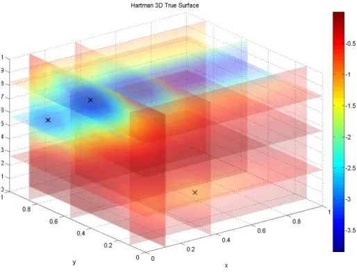
Figure 8: The true response of Hartman 3D function.
3.2.2 3D Hartman Function
Hartman Function has been studied in [4]. The function is defined as :
min f (xj) = − m X i=1 ciexp h − n X j=1 (xj− pij)2 i where m = 4, n = 3, a = 3 10 30 0.1 10 35 3 10 30 0.1 10 35 , c = 1 1.2 3 3.2 , P = 0.3689 0.1170 0.2673 0.4699 0.4387 0.7470 0.1091 0.8732 0.5547 0.0381 0.5743 0.8828 s.t − 2 ≤ x1, x2, x3 ≤ 2 .
There are 3 local minima at (0.1146, 0.5556, 0.8525,), (0.1093, 0.8605, 0.5641), (0.3687, 0.1176, 0.2676). Figure 8 shows the local minima marked by ’x’ on the true surface. We form a grid partition P containing 3375(15 × 15 × 15) grid points.
P = n (x, y)| x ∈ {0, 0 + 1 14, 0 + 2 14, . . . , 1}, y ∈ {0, 0 + 1 14, 0 + 2 14, . . . , 1}, z ∈ {0, 0 + 1 14, 0 + 2 14, . . . , 1} o
We choose 15 initial experimental points by Latin hypercube. In 3D Hartman Function, the limit on the computational cost in the first stage is 5% (3375 × 5% = 168) of all grid points, after that the limit on the computational cost in each stage is 1% (3375 × 1% =
33)of all grid points. The parameters for screening starting points are c1 = 0.35, c2 =
0.5 and c3 = 0.5. The performance of 3D Hartman Function is summarized in Table 10:
Table 10: Performance summary of 3D Hartman Function
Method RT GP PSP TEP NLP
M1 4 282 477 759 3
M2 4 282 402 684 3
M3 5 315 408 723 3
M4 5 311 433 744 3
In Figure 30 to Figure 33, we display the experimental results of M1 to M4. In the
sub-figures, the starting points, the result of APPSPACK, the local extremes, and the explored local extremes are marked as ’X’, ’O’, ’+’, ’4’.
3.3
Comparison
In this section, we compare our multiple stage method with the Multi-Level Single Linkage (MLSL) method [12]. The MLSL method obtains starting points for local search by randomly sampling points within the experimental domain. It generates N new sample points randomly with Latin hypercube in each iteration. In other words, the size of sample points in k-th iteration is kN. Latin hypercube is from the Matlab Optimization Toolbox ( The MathWork 2007a ). Then order kN sample points and choose the rkN sample points as the candidate points. The parameter r ∈ (0, 1] controls the number of candidate
L(x) = R0∞tx−1e−tdt is the gamma function and vol(D) denotes the volume of the
experimental domain D. Both of the critical distance rk and threshold parameter r are
aimed to reduce the starting points for local search.
3.3.1 Multi-Level Single Linkage Method
For the MLSL method, we randomly generate new sample points in each iteration. In this study, N is equal to the number of the experimental grid points in the first stage of our method. For the local search in the MLSL method, we use APPSPACK to find the local extreme of the objective function. For MLSL method, the search region for APPSAPCK is set with the same criterion as our method. Here, two possible criteria can be used for comparison: one is the computation cost of finding the global extreme and another is the computation cost of finding overall local extremes. To compare our method with the MLSL method, this study performs 10 times for each objective function. Experiments involve four different types of functions, including the Ackley Function, MBS Function, Griewank Function, and TGP Function.
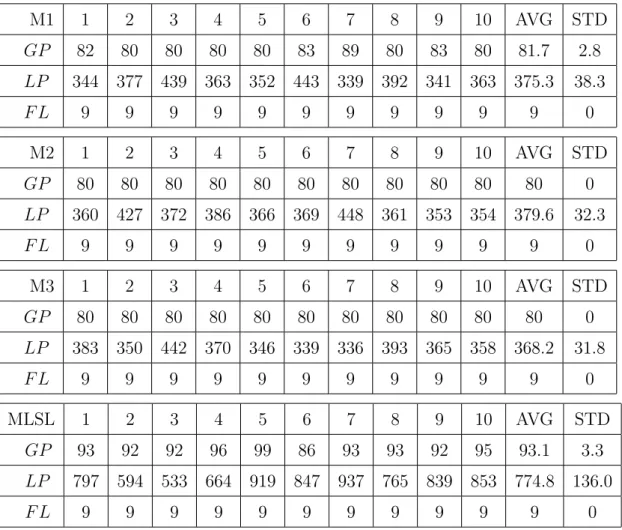
For our method, we use M1, M2, M3 to choose the next possible experimental points. Set the computation cost as 5% of all grid points in the first stage, after that the com-putational cost is 1% of all grid points in each stage. For the MLSL method, the sample points N for Ackley, MBS, Griewank and TGP function are 56, 56, 120 and 600. The number N of sample points for each function are the same as the number of experimental grid points in the first stage of our method, except for TGP function. Because of that, the computational cost of finding overall local extremes with 600 sample points is fewer than 120 sample points according to the experimental results of several trial times. Be-sides, we set r = 50% to choose the candidate points from kN sample points. Table 11, Table 12, Table 13, and Table 14 show the numerical results for these four problems, and the notations are as follow :
N GP : The computational cost of exploring global extreme. N LP : The computational cost of exploring overall local extremes. N FL : The number of identified local extremes.
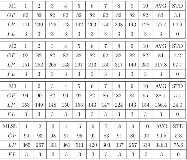
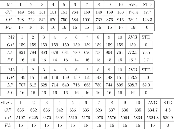
These numerical experiments indicate that regardless of the average computational cost of exploring the global extreme or local extremes, our method performs better than MLSL method, and especially for Griewank function and TGP function. In Griewank function, MLSL method required more than 200 experimental points to identify the global
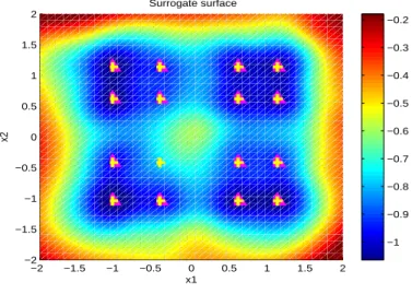
extreme and more than 400 experimental points to identify overall local extremes. In TGP function, M2 could not find some local extremes, because the surrogate surface of the neighborhoods of the unfound local extremes are not good enough. Therefore the possible starting points in this area were not determined as starting points. Figure 9 presents the final surrogate surface of Test10 with M2 , Figure 4 shows the true surface. The local extremes and the explored local extremes are marked as ’+’, ’4’. In spite of
−2 −1.5 −1 −0.5 0 0.5 1 1.5 2 −2 −1.5 −1 −0.5 0 0.5 1 1.5 2 Surrogate surface x1 x2 −1 −0.9 −0.8 −0.7 −0.6 −0.5 −0.4 −0.3 −0.2
Figure 9: The final surrogate surface of Test10 with M2.
this, both of our computational cost are still better than MLSL method. Therefore, These results show that multiple stage method is more efficient in identifying the global extreme and local extremes than the MLSL method.
4
Conclusion
This study proposes a multiple stage method that is modified from two stage method. This multiple stage method combines the advantages of global search methods and local search methods. First, this approach applies a global search method to improve the surrogate surface to simulate the true, unknown response surface in each new stage. The algorithm then selects starting points with the improved surrogate surface using a screening process. Finally, it uses a local search method to explore optimal local extremes with starting points in each new stage. The numerical experimental results of this study indicate that the multiple stage performs better than two stage methods. However, the choice of proper parameters is still a problem in our multiple stage method, especially in
Table 11: Comparison between Our Method and MLSL Method of Ackley
M1 1 2 3 4 5 6 7 8 9 10 AVG STD GP 82 80 80 80 80 83 89 80 83 80 81.7 2.8 LP 344 377 439 363 352 443 339 392 341 363 375.3 38.3 F L 9 9 9 9 9 9 9 9 9 9 9 0 M2 1 2 3 4 5 6 7 8 9 10 AVG STD GP 80 80 80 80 80 80 80 80 80 80 80 0 LP 360 427 372 386 366 369 448 361 353 354 379.6 32.3 F L 9 9 9 9 9 9 9 9 9 9 9 0 M3 1 2 3 4 5 6 7 8 9 10 AVG STD GP 80 80 80 80 80 80 80 80 80 80 80 0 LP 383 350 442 370 346 339 336 393 365 358 368.2 31.8 F L 9 9 9 9 9 9 9 9 9 9 9 0 MLSL 1 2 3 4 5 6 7 8 9 10 AVG STD GP 93 92 92 96 99 86 93 93 92 95 93.1 3.3 LP 797 594 533 664 919 847 937 765 839 853 774.8 136.0 F L 9 9 9 9 9 9 9 9 9 9 9 0Table 12: Comparison between Our Method and MLSL Method of MBS
M1 1 2 3 4 5 6 7 8 9 10 AVG STD GP 82 82 82 82 82 82 92 82 82 82 83 3.1 LP 141 230 126 143 142 263 150 308 143 128 177.4 64.9 F L 3 3 3 3 3 3 3 3 3 3 3 0 M2 1 2 3 4 5 6 7 8 9 10 AVG STD GP 92 82 82 82 82 82 92 82 82 82 84 4.2 LP 151 252 265 143 297 213 150 317 140 250 217.8 67.7 F L 3 3 3 3 3 3 3 3 3 3 3 0 M3 1 2 3 4 5 6 7 8 9 10 AVG STD GP 94 90 82 94 92 82 86 82 84 95 88.1 5.4 LP 153 149 148 150 153 143 147 224 143 154 156.4 24.0 F L 3 3 3 3 3 3 3 3 3 3 3 0 MLSL 1 2 3 4 5 6 7 8 9 10 AVG STD GP 90 93 98 91 95 92 83 91 80 92 90.5 5.3 LP 365 267 301 361 511 420 303 337 257 339 346.1 75.6 F L 3 3 3 3 3 3 3 3 3 3 3 0Table 13: Comparison between Our Method and MLSL Method of
Griewank
M1 1 2 3 4 5 6 7 8 9 10 AVG STD GP 156 164 150 156 156 156 155 156 164 164 174.7 4.7 LP 723 719 761 726 761 692 731 750 760 756 737.9 23.3 F L 17 17 17 17 17 17 17 17 17 17 17 0 M2 1 2 3 4 5 6 7 8 9 10 AVG STD GP 156 156 156 156 156 156 156 156 156 156 156 0 LP 751 736 724 734 746 722 741 730 747 707 733.8 13.5 F L 17 17 17 17 17 17 17 17 17 17 17 0 M3 1 2 3 4 5 6 7 8 9 10 AVG STD GP 156 164 164 164 164 156 156 164 164 164 161.6 3.8 LP 743 727 755 698 758 721 738 764 745 701 735 22.9 F L 17 17 17 17 17 17 17 17 17 17 17 0 MLSL 1 2 3 4 5 6 7 8 9 10 AVG STD GP 160 547 539 640 159 270 147 671 153 582 386.8 226.3 LP 1044 1294 1186 1156 915 1455 1222 1223 892 1144 1153.1 169.4 F L 17 17 17 17 17 17 17 17 17 17 17 0Table 14: Comparison between Our Method and MLSL Method of TGP
M1 1 2 3 4 5 6 7 8 9 10 AVG STD GP 149 244 151 151 151 264 159 148 159 188 176.4 42.7 LP 798 722 842 670 750 584 1001 732 876 916 789.1 123.3 F L 16 16 16 16 16 16 16 16 16 16 16 0 M2 1 2 3 4 5 6 7 8 9 10 AVG STD GP 159 159 159 159 159 159 159 159 159 159 159 0 LP 821 784 863 679 681 780 696 756 904 761 772.5 75.5 F L 16 15 16 14 16 14 16 15 15 15 15.2 0.7 M3 1 2 3 4 5 6 7 8 9 10 AVG STD GP 149 151 159 149 159 159 159 148 148 151 153.2 5.0 LP 707 612 628 714 640 718 665 750 744 809 698.7 62.0 F L 16 16 16 16 16 16 16 16 16 16 16 0 MLSL 1 2 3 4 5 6 7 8 9 10 AVG STD GP 635 632 636 642 636 635 623 637 636 635 634.7 4.8 LP 5107 6225 6370 6301 5619 5176 4976 5576 5064 5834 5624.8 539.9 F L 16 16 16 16 16 16 16 16 16 16 16 0References
[1] D.H. Ackley. A connectionist machine for genetic hillclimbing. 1987.
[2] W.C. Davidon. Variable metric method for minimization. SIAM Journal on Opti-mization, 1:1, 1991.
[3] J.E Dennis and V. Torczon. Direct search methods on parallel machines. SIAM Journal on Optimization, 1991.
[4] L.C.W Dixon and G.P Szego. The global optimization problem: an introduction. Towards global optimization, 2:1–15, 1978.
[5] V.S. Gordon and D. Whitley. Serial and parallel genetic algorithms as function opti-mizers. In Proceedings of the Fifth International Conference on Genetic Algorithms, pages 177–183. Citeseer, 1993.
[6] G.A. Gray and T.G. Kolda. APPSPACK 4.0: asynchronous parallel pattern search for derivative-free optimization. Sandia Report SAND2004-6391, Sandia National Laboratories, Livermore, CA, 2004.
[7] R. Hooke and T.A Jeeves. “Direct Search”Solution of Numerical and Statistical Problems. Journal of the ACM (JACM), 8(2):212–229, 1961.
[8] P.D. Hough, T.G. Kolda, and V.J. Torczon. Asynchronous parallel pattern search for nonlinear optimization. SIAM Journal on Scientific Computing, 23(1):134–156, 2002.
[9] H. Lee. Global Optimization Using Pattern Search and Treed Gaussian Processes. [10] K. M¨uller and L.D. Brown. Location of saddle points and minimum energy paths
by a constrained simplex optimization procedure. Theoretical Chemistry Accounts: Theory, Computation, and Modeling (Theoretica Chimica Acta), 53(1):75–93, 1979. [11] C. Nakazawa, S. Kitagawa, Y. Fukuyama, and H.D. Chiang. A method for searching
multiple local optimal solutions of nonlinear optimization problems. In IEEE Inter-national Symposium on Circuits and Systems, 2005. ISCAS 2005, pages 4907–4910, 2005.
[12] A.H.G. Rinnooy Kan and G.T. Timmer. Stochastic global optimization methods part II: Multi level methods. Mathematical Programming, 39(1):57–78, 1987.
[13] J. Sacks, W.J. Welch, T.J. Mitchell, and H.P. Wynn. Design and analysis of computer experiments. Statistical science, pages 409–423, 1989.
[14] A. Sobester, S.J Leary, and A.J Keane. A parallel updating scheme for approximating and optimizing high fidelity computer simulations. Structural and multidisciplinary optimization, 27(5):371–383, 2004.
[15] V. Torczon. On the convergence of pattern search algorithms. SIAM Journal on Optimization, 1997.
[16] V. Torczon, M.W. Trosset, and Langley Research Center. Using approximations to accelerate engineering design optimization. National Aeronautics and Space Admin-istration, Langley Research Center; National Technical Information Service, distrib-utor, 1998.
[17] W.H. Wang and E.F. Lee. A Two Stage Derivative Free Optimization Method-Warm Starting Points for Local Searches. 2008.
A
Figures
A.1
Ackley Figure
Figure 10: The true and surrogate surface of Ackley with M1
−1.5 −1 −0.5 0 0.5 1 1.5 −1.5 −1 −0.5 0 0.5 1 1.5 7 6 4 2 1 5
Stage1 ackley Surrogate surface "o" −−> final min; "x" −−> starting points(10)
x1 3 9 8 x2 7 8 9 10 11 12 13 14 15 16 17 −1.5 −1 −0.5 0 0.5 1 1.5 −1.5 −1 −0.5 0 0.5 1 1.5
Stage1 ackley True surface "o" −−> final min; "x" −−> starting points(10)
x1 x2 7 8 9 10 11 12 13 14 15 16 17
−1.5 −1 −0.5 0 0.5 1 1.5 −1.5 −1 −0.5 0 0.5 1 1.5
Stage2 ackley Surrogate surface "o" −−> final min; "x" −−> starting points(2)
x1 x2 7 8 9 10 11 12 13 14 15 16 17 −1.5 −1 −0.5 0 0.5 1 1.5 −1.5 −1 −0.5 0 0.5 1 1.5
Stage2 ackley True surface "o" −−> final min; "x" −−> starting points(2)
x1 x2 7 8 9 10 11 12 13 14 15 16 17 −1.5 −1 −0.5 0 0.5 1 1.5 −1.5 −1 −0.5 0 0.5 1 1.5 x1
Stage3 ackley Surrogate surface
x2 7 8 9 10 11 12 13 14 15 16 17
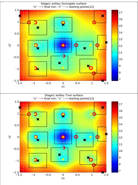
Figure 11: The true and surrogate surface of Ackley with M2 −1.5 −1 −0.5 0 0.5 1 1.5 −1.5 −1 −0.5 0 0.5 1 1.5 5 1 2
Stage1 ackley Surrogate surface "o" −−> final min; "x" −−> starting points(12)
x1 3 6 4 x2 7 8 9 10 11 12 13 14 15 16 17 −1.5 −1 −0.5 0 0.5 1 1.5 −1.5 −1 −0.5 0 0.5 1 1.5
Stage1 ackley True surface "o" −−> final min; "x" −−> starting points(12)
x1 x2 7 8 9 10 11 12 13 14 15 16 17
−1.5 −1 −0.5 0 0.5 1 1.5 −1.5 −1 −0.5 0 0.5 1 1.5 3 1 2
Stage2 ackley Surrogate surface "o" −−> final min; "x" −−> starting points(5)
x1 x2 7 8 9 10 11 12 13 14 15 16 17 −1.5 −1 −0.5 0 0.5 1 1.5 −1.5 −1 −0.5 0 0.5 1 1.5
Stage2 ackley True surface "o" −−> final min; "x" −−> starting points(5)
x1 x2 7 8 9 10 11 12 13 14 15 16 17 −1.5 −1 −0.5 0 0.5 1 1.5 −1.5 −1 −0.5 0 0.5 1 1.5 x1
Stage3 ackley Surrogate surface
x2 7 8 9 10 11 12 13 14 15 16 17
Figure 12: The true and surrogate surface of Ackley with M3 −1.5 −1 −0.5 0 0.5 1 1.5 −1.5 −1 −0.5 0 0.5 1 1.5 7 5 2 1
Stage1 ackley Surrogate surface "o" −−> final min; "x" −−> starting points(12)
x1 3 4 6 x2 7 8 9 10 11 12 13 14 15 16 17 −1.5 −1 −0.5 0 0.5 1 1.5 −1.5 −1 −0.5 0 0.5 1 1.5
Stage1 ackley True surface "o" −−> final min; "x" −−> starting points(12)
x1 x2 7 8 9 10 11 12 13 14 15 16 17
−1.5 −1 −0.5 0 0.5 1 1.5 −1.5 −1 −0.5 0 0.5 1 1.5 1 2
Stage2 ackley Surrogate surface "o" −−> final min; "x" −−> starting points(5)
x1 x2 7 8 9 10 11 12 13 14 15 16 17 −1.5 −1 −0.5 0 0.5 1 1.5 −1.5 −1 −0.5 0 0.5 1 1.5
Stage2 ackley True surface "o" −−> final min; "x" −−> starting points(5)
x1 x2 7 8 9 10 11 12 13 14 15 16 17 −1.5 −1 −0.5 0 0.5 1 1.5 −1.5 −1 −0.5 0 0.5 1 1.5 x1
Stage3 ackley Surrogate surface
x2 7 8 9 10 11 12 13 14 15 16 17
Figure 13: The true and surrogate surface of Ackley with M4 −1.5 −1 −0.5 0 0.5 1 1.5 −1.5 −1 −0.5 0 0.5 1 1.5 6 1 2
Stage1 ackley Surrogate surface "o" −−> final min; "x" −−> starting points(7)
x1 3 4 5 x2 7 8 9 10 11 12 13 14 15 16 17 −1.5 −1 −0.5 0 0.5 1 1.5 −1.5 −1 −0.5 0 0.5 1 1.5
Stage1 ackley True surface "o" −−> final min; "x" −−> starting points(7)
x1 x2 7 8 9 10 11 12 13 14 15 16 17
−1.5 −1 −0.5 0 0.5 1 1.5 −1.5 −1 −0.5 0 0.5 1 1.5
Stage2 ackley Surrogate surface "o" −−> final min; "x" −−> starting points(3)
x1 x2 7 8 9 10 11 12 13 14 15 16 17 −1.5 −1 −0.5 0 0.5 1 1.5 −1.5 −1 −0.5 0 0.5 1 1.5
Stage2 ackley True surface "o" −−> final min; "x" −−> starting points(3)
x1 x2 7 8 9 10 11 12 13 14 15 16 17
−1.5 −1 −0.5 0 0.5 1 1.5 −1.5 −1 −0.5 0 0.5 1 1.5 3 1 Stage3 ackley Surrogate surface "o" −−> final min; "x" −−> starting points(3)
x1 2 x2 7 8 9 10 11 12 13 14 15 16 17 −1.5 −1 −0.5 0 0.5 1 1.5 −1.5 −1 −0.5 0 0.5 1 1.5
Stage3 ackley True surface "o" −−> final min; "x" −−> starting points(3)
x1 x2 7 8 9 10 11 12 13 14 15 16 17
−1.5 −1 −0.5 0 0.5 1 1.5 −1.5 −1 −0.5 0 0.5 1 1.5
Stage4 ackley Surrogate surface "o" −−> final min; "x" −−> starting points(1)
x1 x2 7 8 9 10 11 12 13 14 15 16 17 −1.5 −1 −0.5 0 0.5 1 1.5 −1.5 −1 −0.5 0 0.5 1 1.5
Stage4 ackley True surface "o" −−> final min; "x" −−> starting points(1)
x1 x2 7 8 9 10 11 12 13 14 15 16 17 −1.5 −1 −0.5 0 0.5 1 1.5 −1.5 −1 −0.5 0 0.5 1 1.5 x1
Stage5 ackley Surrogate surface
x2 7 8 9 10 11 12 13 14 15 16 17
A.2
MBS Figure
Figure 14: The true and surrogate surface of MBS with M1
−1.5 −1 −0.5 0 0.5 1 −0.5 0 0.5 1 1.5 2
Stage1 MBS Surrogate surface "o" −−> final min; "x" −−> starting points(10)
x1 1 x2 −150 −100 −50 0 50 100 150 200 250 300 −1.5 −1 −0.5 0 0.5 1 −0.5 0 0.5 1 1.5 2
Stage1 MBS True surface "o" −−> final min; "x" −−> starting points(10)
x1 x2 −150 −100 −50 0 50 100 150 200 250 300
−1.5 −1 −0.5 0 0.5 1 −0.5 0 0.5 1 1.5 2 2 1
Stage2 MBS Surrogate surface "o" −−> final min; "x" −−> starting points(5)
x1 x2 −150 −100 −50 0 50 100 150 200 250 300 −1.5 −1 −0.5 0 0.5 1 −0.5 0 0.5 1 1.5 2
Stage2 MBS True surface "o" −−> final min; "x" −−> starting points(5)
x1 x2 −150 −100 −50 0 50 100 150 200 250 300
−1.5 −1 −0.5 0 0.5 1 −0.5 0 0.5 1 1.5 2
Stage3 MBS Surrogate surface "o" −−> final min; "x" −−> starting points(1)
x1 x2 −150 −100 −50 0 50 100 150 200 250 300 −1.5 −1 −0.5 0 0.5 1 −0.5 0 0.5 1 1.5 2
Stage3 MBS True surface "o" −−> final min; "x" −−> starting points(1)
x1 x2 −150 −100 −50 0 50 100 150 200 250 300
−1.5 −1 −0.5 0 0.5 1 −0.5 0 0.5 1 1.5 2
Stage4 MBS Surrogate surface "o" −−> final min; "x" −−> starting points(1)
x1 x2 −150 −100 −50 0 50 100 150 200 250 300 −1.5 −1 −0.5 0 0.5 1 −0.5 0 0.5 1 1.5 2
Stage4 MBS True surface "o" −−> final min; "x" −−> starting points(1)
x1 x2 −150 −100 −50 0 50 100 150 200 250 300 −1.5 −1 −0.5 0 0.5 1 −0.5 0 0.5 1 1.5 2 x1
Stage5 MBS Surrogate surface
x2 −150 −100 −50 0 50 100 150 200 250 300
Figure 15: The true and surrogate surface of MBS with M2 −1.5 −1 −0.5 0 0.5 1 −0.5 0 0.5 1 1.5 2 2 3
Stage1 MBS Surrogate surface "o" −−> final min; "x" −−> starting points(11)
x1 1 x2 −150 −100 −50 0 50 100 150 200 250 300 −1.5 −1 −0.5 0 0.5 1 −0.5 0 0.5 1 1.5 2
Stage1 MBS True surface "o" −−> final min; "x" −−> starting points(11)
x1 x2 −150 −100 −50 0 50 100 150 200 250 300
−1.5 −1 −0.5 0 0.5 1 −0.5 0 0.5 1 1.5 2
Stage2 MBS Surrogate surface "o" −−> final min; "x" −−> starting points(2)
x1 x2 −100 −50 0 50 100 150 200 250 300 −1.5 −1 −0.5 0 0.5 1 −0.5 0 0.5 1 1.5 2
Stage2 MBS True surface "o" −−> final min; "x" −−> starting points(2)
x1 x2 −100 −50 0 50 100 150 200 250 300
−1.5 −1 −0.5 0 0.5 1 −0.5 0 0.5 1 1.5 2
Stage3 MBS Surrogate surface "o" −−> final min; "x" −−> starting points(2)
x1 x2 −100 −50 0 50 100 150 200 250 300 −1.5 −1 −0.5 0 0.5 1 −0.5 0 0.5 1 1.5 2
Stage3 MBS True surface "o" −−> final min; "x" −−> starting points(2)
x1 x2 −100 −50 0 50 100 150 200 250 300 −1.5 −1 −0.5 0 0.5 1 −0.5 0 0.5 1 1.5 2 x1
Stage4 MBS Surrogate surface
x2 −150 −100 −50 0 50 100 150 200 250 300
Figure 16: The true and surrogate surface of MBS with M3 −1.5 −1 −0.5 0 0.5 1 −0.5 0 0.5 1 1.5 2 2 3
Stage1 MBS Surrogate surface "o" −−> final min; "x" −−> starting points(8)
x1 1 x2 −150 −100 −50 0 50 100 150 200 250 300 −1.5 −1 −0.5 0 0.5 1 −0.5 0 0.5 1 1.5 2
Stage1 MBS True surface "o" −−> final min; "x" −−> starting points(8)
x1 x2 −150 −100 −50 0 50 100 150 200 250 300
−1.5 −1 −0.5 0 0.5 1 −0.5 0 0.5 1 1.5 2
Stage2 MBS Surrogate surface "o" −−> final min; "x" −−> starting points(2)
x1 x2 −100 −50 0 50 100 150 200 250 300 −1.5 −1 −0.5 0 0.5 1 −0.5 0 0.5 1 1.5 2
Stage2 MBS True surface "o" −−> final min; "x" −−> starting points(2)
x1 x2 −100 −50 0 50 100 150 200 250 300 −1.5 −1 −0.5 0 0.5 1 −0.5 0 0.5 1 1.5 2 x1
Stage3 MBS Surrogate surface
x2 −150 −100 −50 0 50 100 150 200 250 300
Figure 17: The true and surrogate surface of MBS with M4 −1.5 −1 −0.5 0 0.5 1 −0.5 0 0.5 1 1.5 2 2 3
Stage1 MBS Surrogate surface "o" −−> final min; "x" −−> starting points(8)
x1 1 x2 −150 −100 −50 0 50 100 150 200 250 300 −1.5 −1 −0.5 0 0.5 1 −0.5 0 0.5 1 1.5 2
Stage1 MBS True surface "o" −−> final min; "x" −−> starting points(8)
x1 x2 −150 −100 −50 0 50 100 150 200 250 300
−1.5 −1 −0.5 0 0.5 1 −0.5 0 0.5 1 1.5 2
Stage2 MBS Surrogate surface "o" −−> final min; "x" −−> starting points(2)
x1 x2 −150 −100 −50 0 50 100 150 200 250 300 −1.5 −1 −0.5 0 0.5 1 −0.5 0 0.5 1 1.5 2
Stage2 MBS True surface "o" −−> final min; "x" −−> starting points(2)
x1 x2 −150 −100 −50 0 50 100 150 200 250 300 −1.5 −1 −0.5 0 0.5 1 −0.5 0 0.5 1 1.5 2 x1
Stage3 MBS Surrogate surface
x2 −150 −100 −50 0 50 100 150 200 250 300
A.3
Griewank Figure
Figure 18: The true and surrogate surface of Griewank with M1
−10 −5 0 5 10 −10 −8 −6 −4 −2 0 2 4 6 8 10 10 12 14 5 2 7 9 8 1
Stage1 Griewank Surrogate surface "o" −−> final min; "x" −−> starting points(14)
x1 3 4 6 11 13 x2 0.5 1 1.5 2 2.5 −10 −5 0 5 10 −10 −8 −6 −4 −2 0 2 4 6 8 10
Stage1 Griewank True surface "o" −−> final min; "x" −−> starting points(14)
x1 x2 0.5 1 1.5 2 2.5
−10 −5 0 5 10 −10 −8 −6 −4 −2 0 2 4 6 8 10 1 Stage2 Griewank Surrogate surface
"o" −−> final min; "x" −−> starting points(3)
x1 2 3 x2 0.5 1 1.5 2 2.5 −10 −5 0 5 10 −10 −8 −6 −4 −2 0 2 4 6 8 10
Stage2 Griewank True surface "o" −−> final min; "x" −−> starting points(3)
x1 x2 0.5 1 1.5 2 2.5 −10 −5 0 5 10 −10 −8 −6 −4 −2 0 2 4 6 8 10 x1
Stage3 Griewank Surrogate surface
x2 0.5 1 1.5 2 2.5
Figure 19: The true and surrogate surface of Griewank with M2 −10 −5 0 5 10 −10 −8 −6 −4 −2 0 2 4 6 8 10 10 12 6 2 3 8 9 1
Stage1 Griewank Surrogate surface "o" −−> final min; "x" −−> starting points(13)
x1 4 5 7 13 11 x2 0.5 1 1.5 2 2.5 −10 −5 0 5 10 −10 −8 −6 −4 −2 0 2 4 6 8 10
Stage1 Griewank True surface "o" −−> final min; "x" −−> starting points(13)
x1 x2 0.5 1 1.5 2 2.5
−10 −5 0 5 10 −10 −8 −6 −4 −2 0 2 4 6 8 10 1 3 Stage2 Griewank Surrogate surface "o" −−> final min; "x" −−> starting points(4)
x1 4 2 x2 0.5 1 1.5 2 2.5 −10 −5 0 5 10 −10 −8 −6 −4 −2 0 2 4 6 8 10
Stage2 Griewank True surface "o" −−> final min; "x" −−> starting points(4)
x1 x2 0.5 1 1.5 2 2.5 −10 −5 0 5 10 −10 −8 −6 −4 −2 0 2 4 6 8 10 x1
Stage3 Griewank Surrogate surface
x2 0.5 1 1.5 2 2.5
Figure 20: The true and surrogate surface of Griewank with M3 −10 −5 0 5 10 −10 −8 −6 −4 −2 0 2 4 6 8 10 10 12 14 6 2 3 8 9 1
Stage1 Griewank Surrogate surface "o" −−> final min; "x" −−> starting points(14)
x1 4 5 7 13 11 x2 0.5 1 1.5 2 2.5 −10 −5 0 5 10 −10 −8 −6 −4 −2 0 2 4 6 8 10
Stage1 Griewank True surface "o" −−> final min; "x" −−> starting points(14)
x1 x2 0.5 1 1.5 2 2.5
−10 −5 0 5 10 −10 −8 −6 −4 −2 0 2 4 6 8 10 1 Stage2 Griewank Surrogate surface
"o" −−> final min; "x" −−> starting points(3)
x1 3 2 x2 0.5 1 1.5 2 2.5 −10 −5 0 5 10 −10 −8 −6 −4 −2 0 2 4 6 8 10
Stage2 Griewank True surface "o" −−> final min; "x" −−> starting points(3)
x1 x2 0.5 1 1.5 2 2.5 −10 −5 0 5 10 −10 −8 −6 −4 −2 0 2 4 6 8 10 x1
Stage3 Griewank Surrogate surface
x2 0.5 1 1.5 2 2.5