國立臺中教育大學教育測驗統計研究所理學碩士論文
指導教授:郭伯臣 博士
基於自適應特徵萃取於高維度資料分類
(Adaptive Feature Extractions
for High Dimensional Data Classification)
研 究 生:林 士 勛 撰
Abstract
In a typical classification process, the size of training data fundamentally affects the
generality of a classifier. Given a finite and fixed size of training data, the
classification result may be degraded as dimensionality increasing. Many researches
have demonstrated that multiple classifiers can alleviate small sample size and high
dimensionality concern such that the effect is better than single model. The effective
method for generating diverse classifiers is adaptive boosting method (AdaBoost). In
this thesis, we propose a novel multiple feature space to train diverse classifiers, and
name adaptive feature extractions which are divided into three parts. First, the scatter
matrices between feature vectors are explored by feature extractions, and apply
AdaBoost into feature extraction to generate multiple feature space. In these multiple
feature space, training diverse classifiers, and applying weighted vote method to
combine these classifiers to enhance the effect of identification. Second, AdaBoost has
the advantage of generating various classifiers. However, the disadvantage is that
increasing the weights of misclassified samples and the outliers are also incorporated.
In this thesis, using the samples of the reject region to replace the misclassified
samples can avoid this problem. Third, the concept of neighborhood system method is
applied to train spatial classifiers. In each iteration, we will train two kinds of
classifiers (spectral and spatial classifiers) and reserve a good performance classifier.
Finally, these various classifiers are combining by weighted vote. The Gaussian and
knn classifiers are used to train multiple classifiers. The experimental results show that
our novel methods can get good results of high dimensional data classification.
摘 要
在典型的辨識過程中,訓練樣本數的多寡影響著辨識器的優劣甚鉅。在給定有限 且固定樣本數的條件下,辨識率往往反而會因為維度數的增加而下降,這也就是 常見的 Hughes 現象或者稱之為維度詛咒。許多研究已經證實出可藉由多重辨識 器(multiple classifiers)來減緩小樣本高維度的顧慮,並且能夠得到比單一辨識器更 好的辨識效果,其中一個有效的方法便是建構一群具有多樣性的辨識器(diverse classifiers),如普適提(Adaptive Boosting, AdaBoost)。本研究將提出一個新穎的多重特徵空間來訓練多樣化辨識器,我們將這個方法命名為自適應特徵萃取法,其 中分成了三個部分。首先,我們將藉由分散矩陣(scatter matrices)來探究特徵向量 間的關聯性,並且應用 AdaBoost 結合特徵萃取迭代生成多重特徵空間(multiple feature space),在這些多重空間中訓練辨識器,最後再利用加權合成辨識器的技 巧,來提升辨識的效果;因為 AdaBoost 是加重錯誤點的權重,但有些錯誤點則 是離群點(outlier),會影響參數估計的準確度,我們融入拒絕域(reject region)的概 念可避免取到離群點;最後融入鄰域系統(neighborhood system)的概念,訓練光譜 或空間資訊的分類器,再將這些分類器做加權合成。在此文章中,使用 Gaussian 辨識器和 knn 無參數辨識器,來訓練生成多重辨識器,且分析辨識效果成效。由 實驗的結果顯示,本研究提出的自適應特徵萃取法,獲得更好的辨識效果。 關鍵字:普適提、特徵萃取、鄰域系統、拒絕域
Table of Contents
CHAPTER 1: INTRODUCTION... 1
1.1 Statement of Problem...
2
1.2 Organization of Thesis ...
6
CHAPTER 2: LITERATURE REVIEW... 7
2.1 Hughes Phenomenon...
7
2.2 Adaptive Boosting Algorithm ...
9
2.3 Nonparametric Weighted Feature Extraction...
10
2.4 Reject Region ...
13
2.4.1 Likelihood Ratio Reject Options...
13
2.4.2 k Nearest Neighbors Reject Options ...
15
2.5 Neighborhood System ...
16
2.6 Classifiers ...
18
2.6.1 Gaussian classifier ...
20
2.6.2 k-nearest-neighbor classifier...
20
CHAPTER 3: ADAPTIVE FEATURE EXTRACTIONS ... 23
3.1 Introduction ...
23
3.2 Adaptive Feature Extractions ...
24
3.2.1 An Adaptive Feature Extraction Based on Classification Error...
24
3.2.2 An Adaptive Feature Extraction with Reject Region ...
28
CHAPTER 4: DATA SETS AND EXPERIMENTAL RESULTS... 35
4.1 Hyperspectral Image Dataset and Experiments...
35
4.1.1 Data Description ...
35
4.1.2 Experimental Designs and Results ...
36
4.2 Educational Measurement Dataset and Experiments...
47
4.2.1 Data Description ...
47
4.2.2 Experimental Designs and Results ...
49
4.3 UCI Datasets and Experiments ...
52
4.3.1 Data Description ...
52
4.3.2 Experimental Designs and Results ...
52
CHAPTER 5: CONCLUSION AND FUTURE WORK ... 57
5.1 Conclusion ...
57
5.2 Suggestions for Future Work...
58
APPENDIX A: THE TEST OF “SECTOR” UNIT ... 59
List of Tables
Table 2.1. The algorithm of adaptive boosting ...
9
Table 2.2. The algorithm of nonparametric weighted feature extraction ...
12
Table 3.1. The algorithm of adaptive feature extraction based on classification
error...
27
Table 3.2. The algorithm of adaptive feature extraction with reject region ...
29
Table 3.3. The algorithm of adaptive feature extraction with spatial information ...
32
Table 4.1. Number of pixels for each category in the Washington DC Mall Image ...
36
Table 4.2. The accuracy of Case 1, Case 2, and Case 3 ...
37
Table 4.3. Six categories of remedial instructions ...
48
Table 4.4. The number of training subjects and testing subjects of the experiment ...
49
Table 4.5. The accuracy of four methods with two classifiers in educational
testing experiment ...
50
Table 4.6. The datasets of UCI Machine Learning Repository...
52
Table 4.7. The accuracy of four methods with two classifiers in UCI datasets
List of Figures
Figure 1.1. The schematic image of original spectrum ...
1
Figure 1.2. A schematic diagram for high dimensional data classification ...
2
Figure 2.1. Hughes phenomenon ...
9
Figure 2.2. The relationship between sample points and their local means ...
12
Figure 2.3. The first-order neighborhood system ...
17
Figure 2.4. The second-order neighborhood system. ...
17
Figure 2.5. An example of Bayes decision rule in one-dimensional space ...
19
Figure 2.6. knn decision rule...
21
Figure 3.1. The main idea of adaptive feature extraction ...
24
Figure 3.2. The flowchart of AdaFE based on classification error ...
25
Figure 3.3. The flowchart of AdaFE with reject region ...
28
Figure 3.4. The flowchart of AdaFE with spatial information ...
31
Figure 4.1. Washington DC Mall Image...
36
Figure 4.2. The accuracy of five methods with Gaussian classifier for hyperspectral image classification in Case 1 ...
38
Figure 4.3. The accuracy of five methods with kNN (k=3) classifier for hyperspectral image classification in Case 1 ...
38
Figure 4.4. The accuracy of five methods with Gaussian classifier for
hyperspectral image classification in case 2 ...
39
Figure 4.5. The accuracy of five methods with kNN (k=3) classifier for hyperspectral image classification in Case 2 ...
39
Figure 4.6. The accuracy of five methods with Gaussian classifier for hyperspectral image classification in case 3 ...
40
Figure 4.7. The accuracy of five methods with kNN (k=3) classifier for hyperspectral image classification in Case 3 ...
40
Figure 4.8. Washington DC Mall Image ...
42
Figure 4.9. (a) NonFE with Gaussian classifier in cases 3 ...
42
Figures 4.9. (b)-(d) NWFE with Gaussian classifier in cases 1, 2, and 3...
42
Figures 4.10. (a)-(c) AdaFE_CE with Gaussian classifier in cases 1, 2, and 3 ..
43
Figures 4.10. (d)-(f) AdaFE_RR with Gaussian classifier in cases 1, 2, and 3 ..
43
Figures 4.11. (a)-(c) AdaFE_SI with Gaussian classifier in cases 1, 2, and 3....
44
Figures 4.11. (d)-(f) NonFE with kNN (k=3) classifier in cases 1, 2, and 3 ...
44
Figures 4.12. (a)-(c) NWFE with kNN (k=3) classifier in cases 1, 2, and 3 ...
45
Figures 4.12. (d)-(f) AdaFE_CI with kNN (k=3) classifier in cases 1, 2, and 3 .45
Figures 4.13. (a)-(c) AdaFE_RR with kNN (k=3) classifier in cases 1, 2, and 3Figure 4.14. Experts’ structure of “Sector” unit ...
47
Figure 4.15. The accuracy of four methods with Gaussian classifier ineducational testing experiment...
51
Figure 4.16. The accuracy of four methods with kNN (k=3) classifier ineducational testing experiment...
51
Figure 4.17. The accuracy of four methods with Gaussian classifier in Glassdataset experiment...
54
Figure 4.18. The accuracy of four methods with kNN (k=3) classifier in Glassdataset experiment...
54
Figure 4.19. The accuracy of four methods with Gaussian classifier in Heartdataset experiment...
55
Figure 4.20. The accuracy of four methods with kNN (k=3) classifier in Heartdataset experiment...
55
Figure 4.21. The accuracy of four methods with Gaussian classifier in Yeastdataset experiment...
56
Figure 4.22. The accuracy of four methods with kNN (k=3) classifier in YeastCHAPTER 1: INTRODUCTION
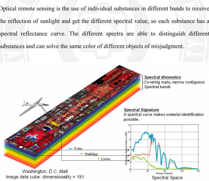
Remote sensing is a way to use sensors in the case of objects without touching the target to collect information. In order to collect a wide range of information, the airplane or satellite will carry sensors into the air toward the ground, sea and atmosphere to conduct detection. The collected information will be used for analysis. Optical remote sensing is the use of individual substances in different bands to receive the reflection of sunlight and get the different spectral value, so each substance has a spectral reflectance curve. The different spectra are able to distinguish different substances and can solve the same color of different objects of misjudgment.
1.1 Statement of Problem
Presently, high dimensional data are used generally such as hyperspectral image data classification, face recognition, handwritten character recognition, and gene expression data classification in bioinformatics. Pattern recognition is the thesis of how machines can observe the environment, learn to distinguish patterns of interest from their background, and make sound and reasonable decisions about the categories of the patterns. Among the ways to approach high dimensional data classification, a useful processing model (Landgrebe, 1999) that has evolved in the recent years is shown schematically in Figure 1.2. Given the availability of data (box 1), the process begins by the analyst specifying what classes are desired, usually by labeling training samples for each class (box 2). New elements that have proven important in the case of high dimensional data are those indicated by boxes in the diagram marked 3, 4 and 5. These are the focus of this thesis and will be discussed in more detail shortly; however the reason for their importance in this context is as follows.
4. Feature Extraction
or Feature Selection 5. Classifier 2. Label Training Samples
1. Hyperspectral Data
(Training Samples) 6. Output
3. Determine Quantitative Class Descriptions
Classification techniques in pattern recognition typically assume that there are enough training samples available to obtain reasonably accurate class descriptions in quantitative form. Unfortunately, the number of training samples required to train a classifier for high dimensional data is much greater than that required for conventional data, and gathering these training samples can be difficult and expensive. Consequently, the assumption that enough training samples are available to accurately estimate the class quantitative description is frequently not satisfied for high dimensional data. We often face the small sample size problems in the real situation which causes Hughes phenomenon or the curse of dimensionality (Hughes, 1968; Bellman, 1961; Raudys & Jain, 1991), and it usually makes a single classifier weak and has large variances in classification results. Many researches have demonstrated that multiple classifiers can alleviate small sample size and high dimensionality concern, and obtain more outstanding and robust results than single models. One of the effective approaches for generating an ensemble of diverse base classifiers is the use of different feature space such as adaptive boosting method (AdaBoost) (Freund & Schapire, 1997).
AdaBoost (Freund & Schapire, 1997) creates a collection of component classifiers by maintaining a set of weights over training samples and adaptively adjusting these weights after each boosting iteration: the weights of the training samples which are misclassified by current component classifier will be increased while the weights of the training samples which are correctly classified will be decreased. AdaBoost is based on the decision tree classifier, but it may not be extended to all kinds of classifiers. And if adding feature extraction to do iteration in this ensemble, then reducing the number of iterations and increasing the recognition rate.
Some studies (Hsieh, Wang, & Hsu 2006; Song, Fan, & Rao, 2005; Richards, 2005; Landgrebe, 2005) have shown that nonparametric weighted feature extraction (NWFE) (Kuo, 2004) is powerful to reduce the dimensionality of hyperspectral image data. However, if the transformed samples are mixed, then the classifier can not discriminate these samples correctly.
Recently, the classification technique integrating both spectral and spatial information has mushroomed for the hyperspectral image classification (Solberg, Taxt, & Jain, 1996; Tso & Mather, 1999; Rellier, Descombes, Falzon, & Zerubia, 2004; Li & Narayanan, 2004; Cossu, Chaudhuri, & Bruzzone, 2005; Jia & Richards, 2008), where Markov random field (MRF) (Kinderman & Snell) is one of the popular models to exploit spatial-context between neighboring pixels in an image.
The objectives of this research are:
1. The scatter matrices between feature vectors are explored by feature extractions, and apply AdaBoost into feature extraction to generate multiple feature space. In these multiple feature space, training diverse classifiers, and applying weighted vote to combine these classifiers to enhance the effect of identification.
2. AdaBoost has the advantage of generating various classifiers. However, the disadvantage is that increasing the weights of misclassified samples, the outliers are also incorporated. In this thesis we propose to apply the samples of the reject region (Kuo, 2003; Ko, 2005) to replace the misclassified
3. A novel classification processing based on the spatial information and the concept of Adaboost for hyperspectral image classification is proposed. This classification process is named adaptive feature extraction with spatial information. The main idea is adaptive in the sense that subsequent feature spaces are tweaked in favor of those instances misclassified by spectral or spatial classifiers in the previous feature space.
1.2 Organization of Thesis
Chapter 1: A statement of the problem and the purpose of this research are described. Chapter 2: The literature reviews are about the Hughes phenomenon, nonparametric
weighted feature extraction (NWFE) that is used to reduce features, adaptive boosting that is applied to the multiple classifiers, reject region, neighborhood system, and classifiers.
Chapter 3: A novel ensemble method for the dimensionality reduced and doing iteration. This new concept is deduced from adaptive boosting, nonparametric weighted feature extraction and reject region. In addition, a novel classification processing based on the spatial information and the concept of Adaboost for hyperspectral image classification is proposed. Chapter 4: The experimental designs and results (hyperspectral image dataset,
educational testing dataset, and UCI dataset) represent from the process of the ensemble construction.
Chapter 5: General conclusions and potentials for future research development are suggested in this chapter.
CHAPTER 2: LITERATURE REVIEW
For supervised classification, the accuracy of the classification rule often depends on the number of training samples. The more training samples, the more accurately a generalized description of data classes can be obtained. Consequently, a more robust classifier may be constructed. Unfortunately, gathering enough training samples is such a difficult and expensive task that facing the circumstance with insufficient training samples is often inevitable. In this chapter, we will briefly introduce the Hughes phenomenon in section 2.1. The adaptive boosting (AdaBoost) algorithm, nonparametric weighted feature extraction (NWFE), reject region method, neighborhood system method (Kinderman & Snell), and the learning algorithms of classifiers are introduced in sections 2.2, 2.3, 2.4, 2.5, and 2.6, respectively.
2.1 Hughes Phenomenon
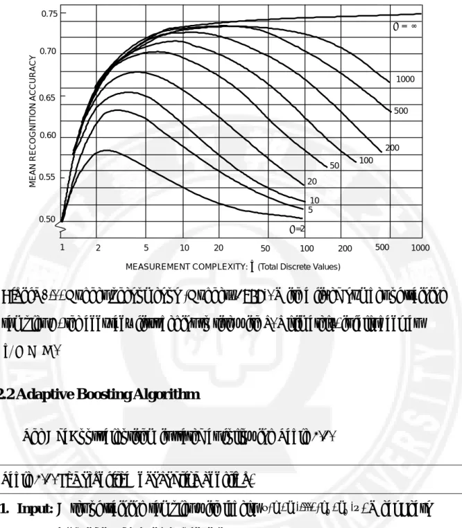
Hughes phenomenon (Hughes, 1968), as seen in Figure 2.1, commonly occurs in classification issues, when the number of training samples is small compared to the number of features. Although increasing the number of features can offer the potential to discriminate more detail classes, this positive effect is gradually diluted by poor parameter estimation. Consequently, the subsequent classifier performance is weak and less accurate than need be. This paradoxical behavior is also referred to as the curse of dimensionality, or the peaking phenomenon (Bellman, 1961; Raudys & Jain,
1991). In literatures the term “weak classifier” can refer to several things (Skurichina & Duin, 2002): badly performing classifiers, unstable classifiers, classifiers of a low complexity, or classifiers depending upon certain assumed models that are not always true. Generally, “weak classifier” we mention here is that the one has an unsatisfying performance.
In order to overcome the Hughes phenomenon and to improve the performance of a weak classifier constructed on small training sample sizes, one may use different approaches which can be categorized into three groups. First, one may reduce the dimensionality but lose discrimination power as small as possible at the same time via feature extraction and feature selection. Some of the commonly used methods for feature extraction are principal component analysis (PCA) (Fukunaga, 1990), Fisher’s linear discriminant analysis (LDA) (Fukunaga, 1990), nonparametric weight feature extraction (NWFE) (Kuo & Landgrebe, 2004), etc.; Second, it is possible to stabilize the decision of a classifier by regularizing the sample covariance matrix (Friedman, 1989). Third, instead of looking for the best set of features or the best single classifier, another approach is to construct a set of classifiers and then to combine them into a powerful decision rule (Kuncheva, 2004).
Figure 2.1. Hughes phenomenon (Hughes, 1968). With a fixed number of training
samples N, the accuracy first begins to rise with d. Ultimately, it falls back as
N
n .
2.2 Adaptive Boosting Algorithm
The AdaBoost algorithm is stated as following Table 2.1. Table 2.1. The algorithm of adaptive boosting.
1. Input: A set of training samples with labels {(x1,y1),...,(xN,yN)}, WeakLearn
algorithm, the number of cycles T.
2. Initialize: The weight of samples: wi 1N
1 , for all i1,...,N.
3. Do for t 1,...,T
(1) Use WeakLearn algorithm to train the weak learner ht on the weighted
training sample set.
MEASUREMENT COMPLEXITY: n (Total Discrete Values)
1 2 5 10 20 50 100 200 500 1000 0.50 0.55 0.60 0.65 0.70 0.75 N=2 5 10 20 50 100 200 1000 500 N = ∞ MEAN RECOGN ITION ACCURA CY
(2) Calculate the training error of iN1 t, i t( i)
i t
t:ε w y h x
h
.(3) Set weight of weak learner ht:αt ln((1-εt)/εt). (4) Update training sample’s weights:
t i t i t t i t i Z x h y -α w w1 exp{ ( )} , where Zt is
a normalization constant, and
1 1 1 N i t i w . 4. Output:
f
(
x
)
sign
(
tT1α
th
t(
x
)
)
.Adaptive boosting (AdaBoost) (Freund & Schapire, 1997) is an iterative machine learning procedure and one popular method with many successful applications. Its purpose is to find a highly accurate classification rule by combining many weak or base classifiers, many of which may be only moderately accurate. At boosting processes, training samples and their corresponding labels that are easy to classify get lower weights. The intended effect is to force the base classifier to concentrate on “difficult to identify” samples with high weights, which will be effective to the overall goal of finding a highly accurate classification rule.
2.3 Nonparametric Weighted Feature Extraction
NWFE is a nonparametric feature extraction. The main ideas of NWFE are putting different weights on every sample to compute the “local means” and defining new nonparametric between-class and within-class scatter matrices to get more features. In NWFE, the nonparametric between-class scatter matrix is defined as
L i L i j j N T i j i i j i i j i i NW b i x M x x M x N P S 1 1 1 ) ( ) ( ) ( ) ( ) , ( ) ) ( ( ) ) ( ( . (2.1)The nonparametric within-class scatter matrix is defined as
T i i i L i N i i i i i i i NW w x M x x M x N P S i ( ( ))( () ( ()) ) 1 1 ) ( ) ( ) , (
, (2.2) where (i) kx refers to the k-th sample from class i. The scatter matrix weight ( ji, )
k is defined as
j n l i l j i l i k j i k j i k x M x dist x M x dist 1 1 ) ( ) ( 1 ) ( ) ( ) , ( )) ( , ( )) ( , ( , (2.3)where dist( ba, ) means the distance from a to b. And ( (i))
k j x
M is the local mean of
) (i
k
x in the class j and defined as
Ni l j l j i l i k j x w x M 1 ) ( ) , ( ) ( ) ( , (2.4) where
j N l j l i k j l i k j i l x x dist x x dist w 1 1 ) ( ) ( 1 ) ( ) ( ) , ( ) , ( ) , ( . (2.5)The optimal features are determined by optimizing the criteria given by ] ) [( ) ( 1 NW b NW w NWFE p tr S S J . (2.6)
Table 2.2. The algorithm of nonparametric weighted feature extraction.
1. Compute the distances between each pair of sample points and form the distance matrix.
2. Compute ( ji, )
l
w using the distance matrix. 3. Use ( ji, )
l
w to compute local means ( (i))
k j x
M .
4. Compute scatter matrix weight ( ji, )
k . 5. Compute NW b S and NW w S .
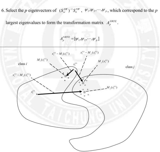
6. Select the p eigenvectors of NW b NW w S S ) 1 ( , p
1, 2,, , which correspond to the p
largest eigenvalues to form the transformation matrix NWFE p A . ] , , , [ 1 2 p NWFE p A ) ( () ) ( i t j i t M x x ( )i t x ) ( (i) t j x M ) ( (i) l i x M ) ( () ) ( i l i i l M x x ) (i l x ) ( () ) ( i l j i l M x x ) ( (i) l j x M class i class j
Figure 2.2 is the representation of NWFE between-class and within-class scatter matrices in the distributions of classes are nonnormal-like distributions. It shows the importance of using boundary points and local means.
2.4 Reject Region
2.4.1 Likelihood Ratio Reject Options
Suppose X is a d-dimensional random vector and x1,x2,,xN are N training
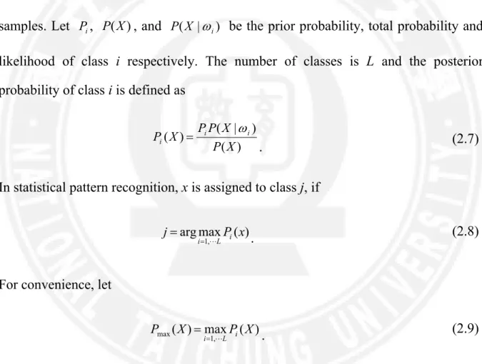
samples. Let Pi, P(X), and P(X | be the prior probability, total probability and i)
likelihood of class i respectively. The number of classes is L and the posterior probability of class i is defined as
) ( ) | ( ) ( X P X P P X P i i i . (2.7)
In statistical pattern recognition, x is assigned to class j, if ) ( max arg , 1 P x j i L i . (2.8)
For convenience, let
) ( max ) ( , 1 max X P X P i L i . (2.9)
The definition of reject patterns (RP) with rejection threshold r in (Giusti, Masulli, & Sperduti., 2002) and (Chow, 1970) is
} ) ( | { ) (r x Pmax x r RP . (2.10)
The patterns of reference database (RD) of with threshold are in } ) ( | { ) ( x Pmax x RD . (2.11)
In (Giusti, Masulli, & Sperduti., 2002), the rejection threshold r and the reference database threshold can be different; hence the rejected training patterns of samples may be different from the reference database patterns for second stage classification. In this thesis, another approach based on the likelihood ratio of different classes is used to measure the “confusedness” and then define the rejected patterns.
Let the likelihood ratio of class i and j be
j i x P x P x P x P x LR i j j i ij , where ( ) ( ) ,and ) ( ) ( ) ( (2.12)
then the number of proposed likelihood ratios is L-1. By sorting them in increasing order, we can have
) ( ) ( ) ( 1 LR(1) x LR(2) x LR(L1) x . (2.13)
The following mean of likelihood ratios is used to measure the confusedness of pattern
x in this thesis. L S x LR S S x LR S s s 1 , 1 where ), ( 1 ) , ( ( ) 1
(2.14)) , ( ) , ( ) , (x(1) S LR x(2) S LR x( ) S LR N . (2.15)
Then the reject set (RS) with reject rate R is defined as } , , , { ) (R x(1) x(2) x([RN]1) RS . (2.16)
2.4.2 k Nearest Neighbors Reject Options
Suppose X is a d-dimensional random vector and x1,x2,,xN are N training
samples. fi(x) is the frequency of class i among k neighbors in the training set to a
testing sample x and must satisfy that
k x f L i i
1 ) ( (2.17)where L is the number of classes. In k nearest neighbors classification, x is assigned to class j, if ) ( max arg , 1 f x j i L i . (2.18)
In this thesis, another definition based on the ratio of frequency of different classes is used to measure the “confusedness” and then define the rejected patterns. Let the ratio of frequencies of different classes of class i and j be
j i x f x f x f x f x FR i j j i ij , where ( ) ( ) ,and ) ( ) ( ) ( (2.19)
then the number of proposed frequency ratios is L-1. By sorting them in increasing order, we can have
1 ) ( ) ( ) ( (2) ( 1) ) 1 ( x FR x FR x FR L . (2.20)
The following mean of frequency ratios is used to measure the confusedness of pattern x in this thesis.
L S x FR S S x FR S s s ( ), where 1, 1 1 ) , ( 1 ) (
(2.21)The mean is closer to 1, the rejection degree of pattern x is greater. Suppose that the number of rejected patterns is RN, where R is the reject rate between 0 and 1. Let
) ( ) 2 ( ) 1 ( ,x , ,xN
x be the sorted array with
) , ( ) , ( ) , (x(1) S FR x(2) S FR x( ) S FR N . (2.22)
Then the reject set (RS) with reject rate R is defined as
} , , , { ) (R x(1) x(2) x([RN]1) RS . (2.23) 2.5 Neighborhood System
In the image data X, each grid location on the conditional probability only with its neighbors (Neighborhood) related to the known Markov random field (MRF) (Kinderman & Snell, 1980). Support
x1,x2,xN
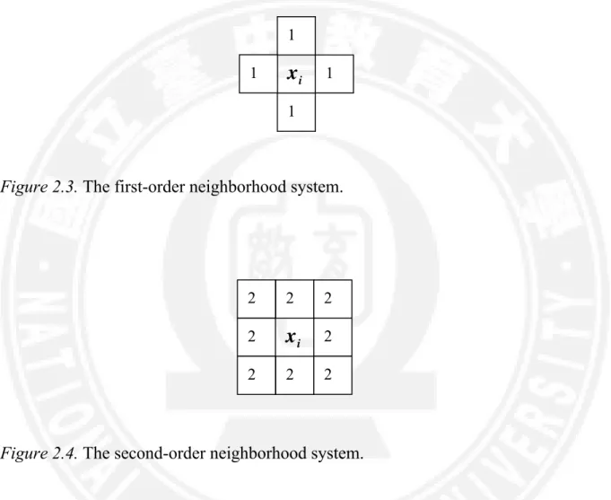
dimension space defined on N numbers of variables while MRF is basis and neighborhood relationship construct its space information conditional probability:Where Ni is xi's neighbor set (neighborhood set). The neighbor set can be defined
as n-order neighbors in the image grid space. Figure 2.3 and Figure 2.4 are the first- and second-order neighborhood systems.
Figure 2.3. The first-order neighborhood system.
Figure 2.4. The second-order neighborhood system.
Hammersley and Clifford proved that any MRFs are equivalent to the Gibbs distribution. In the other word, if xiis a Markov random field then xi would follow the
Gibbs distribution (Hammersley & Clifford, 1971). The Gibbs distribution is defined as follows:
C c c x V Z x ) exp ( ) P( 1 , (2.25) 2 2 2 2 2 2 2 2 ix
1 1 1x
i 1where Z is a normalization constant such that
( )1X X x
P ; )Vc(x is a potential function.
For any set of clique c = {s, t} defined as follows:
) ( ) ( c s t c x u u V , (2.26)
where c is the adjust parameter in the clique c.
2.6 Classifiers
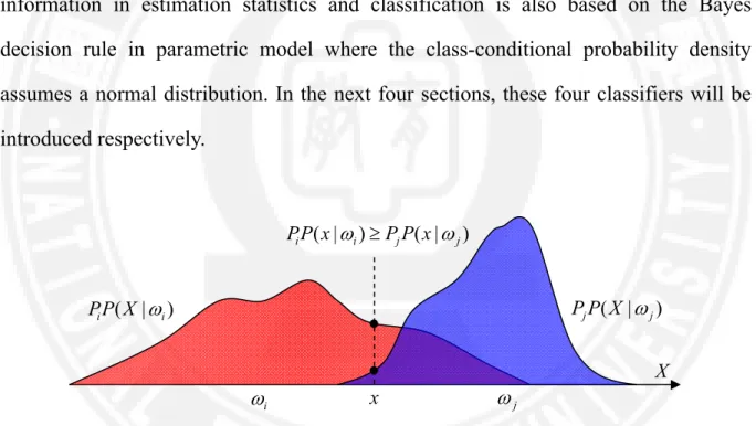
Once the dimensionality reduction techniques or other pre-processing procedures modify the original data to a proper representation, a classifier can be constructed by using a number of possible learning algorithms where the Bayes decision rule is one of the most commonly used decision rules.
The main concept of Bayes decision rule is based on the probabilistic approach using Bayes theorem. An input sample x can be assigned to one of the L-class
} , , ,
{1 2 L which maximizes a posterior probability (MAP):
)} | ( { max arg } , , 2 , 1 { x P i L i MAP , (2.27)
where the posterior probability P(i|x) may be calculated from prior probability Pi
and the class-conditional density function P(x| , using Bayes theorem, as i)
L i i i i i i x P P x P P x P 1 ) | ( ) | ( ) ( . (2.28)optimization, formula (2.27) can be simplified as )} | ( { max arg } , , 2 , 1 { L i i i MAP PP x . (2.29)
The density estimate can be categorized into either parametric or nonparametric model. Some well-known classifiers based on Bayes decision rule are Gaussian classifier in parametric model and k-nearest-neighbor classifier and Parzen classifier in nonparametric models. Additionally, in hyperspectral image classification, a Markov random field-based contextual classification utilizing both spectral and spatial information in estimation statistics and classification is also based on the Bayes decision rule in parametric model where the class-conditional probability density assumes a normal distribution. In the next four sections, these four classifiers will be introduced respectively.
Figure 2.5. An example of Bayes decision rule in one-dimensional space. In this
case, the input sample x is assigned to class i according to formula (2.29).
There are still two types of classifiers commonly applied as the base classifier in multiple classifier systems: decision tree classifier and support vector machine. The decision rules of them are to find the separating hyperplane(s) by selecting the most salient feature at each node of the tree and by maximizing the margin been defined by
X ) | ( i iP X P PjP(X |j) i x ) | ( ) | ( i j j iP x PP x P j
the support vectors, respectively. These two classifiers are introduced in the last two sections of this chapter.
2.6.1 Gaussian classifier
Gaussian classifier (GC) is made up of the assumption that the samples are drawn from a multivariate normal population with mean and covariance matrix . Hence, the class-conditional probability density function can be represented as follows (Fukunaga, 1990). )} ( 2 1 exp{ | | ) 2 ( 1 ) | ( 2 2 1 2 x d x P i n i (2.30) where 2( ) ( ) 1( ) i i T i x M M x x d . (2.31)
Moreover, the MAP estimate (2.29) in connection with Equations (2.30) and (2.31) becomes as MAP ( ) ( )} 2 1 exp{ | | ) 2 ( 1 { max arg 1 2 1 2 } , , 2 , 1 { i i T i i n i L i M x M x P .} ) ( ) ( ln ln 2 { min arg 1 } , , 2 , 1 { const M x M x P T i i i i i L i (2.32)
Here, the term const. does not depend on the particular class assignment.
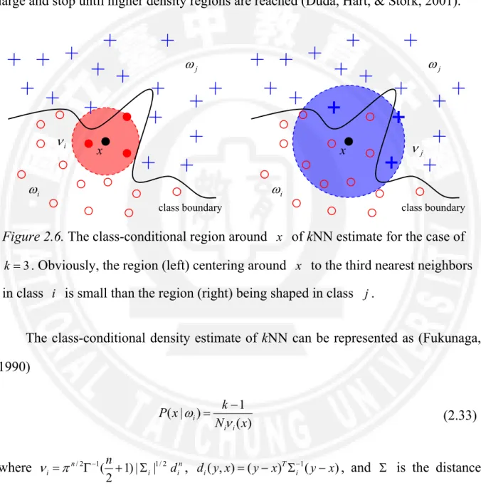
most frequent class among this set. On the probability perspective, the kNN rule is to extend the local region around x until the kth nearest neighbors is found; hence, we have that if the density is high around x, the region is relatively small which provides good solution. On the contrary, if the density is low, the region will grow large and stop until higher density regions are reached (Duda, Hart, & Stork, 2001).
Figure 2.6. The class-conditional region around x of kNN estimate for the case of
3
k . Obviously, the region (left) centering around x to the third nearest neighbors in class i is small than the region (right) being shaped in class j.
The class-conditional density estimate of kNN can be represented as (Fukunaga, 1990) ) ( 1 ) | ( x N k x P i i i (2.33) where n i i n i d n 1/2 1 2 / 1)| | 2 ( , d(y,x) (y x) 1(y x) i T i
, and is the distance
metric. i j class boundary x j i j class boundary x i
Therefore, the MAP estimate (2.29) using the class-conditional distribution of kNN becomes MAP } ) ( 1 { max arg } , , 2 , 1 { N x k P i i i L i ))} , ( | | ) 1 2 ( ln( ) 1 ln( ln { min arg /2 1 1/2 () } , , 2 , 1 { x x d n N k P i NN k n i i n i i L i i .} ) , ( ln | | ln 2 1 ln ln { min arg () } , , 2 , 1 { const x x d n N P i NN k i i i i L i i (2.34)
CHAPTER 3: ADAPTIVE FEATURE EXTRACTIONS
3.1 Introduction
In a typical classification process, the size of training data fundamentally affects the generality of a classifier. Given a finite and fixed size of training data, the classification result may be degraded as dimensionality increasing. Many researches have demonstrated that multiple classifier system can alleviate small sample size and high dimensionality concern such that the effect is better than single model. In this section, we presents three novel methods as following. First, the scatter matrices between feature vectors are explored by feature extractions, and apply AdaBoost with feature extraction of multiple feature space iterative produce. In these multiple feature space, training diverse classifiers, and applying weighted vote method to combine these classifiers to enhance the effect of identification. Second, AdaBoost has the advantage of generating various classifiers. However, the disadvantage is that increasing the weights of misclassified samples, the outliers are also incorporated. In this problem, using the samples of reject region to replace the misclassified samples can avoid this problem. Third, the concept of neighborhood system method is applied to train spatial classifiers. In each iteration, we will train two kinds of classifiers (spectral and spatial classifiers) and reserve a good performance classifier. Finally, these various classifiers are combining by weighted vote.
3.2 Adaptive Feature Extractions
The main idea of adaptive feature extraction (AdaFE) is to find a suitable feature space for those data which are difficult to identify in the previous feature space.
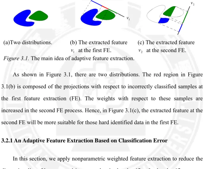
(a)Two distributions. (b) The extracted feature
1
v at the first FE.
(c) The extracted feature
2
v at the second FE.
Figure 3.1. The main idea of adaptive feature extraction.
As shown in Figure 3.1, there are two distributions. The red region in Figure 3.1(b) is composed of the projections with respect to incorrectly classified samples at the first feature extraction (FE). The weights with respect to these samples are increased in the second FE process. Hence, in Figure 3.1(c), the extracted feature at the second FE will be more suitable for those hard identified data in the first FE.
3.2.1 An Adaptive Feature Extraction Based on Classification Error
In this section, we apply nonparametric weighted feature extraction to reduce the dimensionality of hyperspectal image, and train the classifier. In the classifier aspect, we set the weight for the classifier by the misclassified rate of this classifier. In the feature extraction aspect, we increase the weight for the scatter matrices of the misclassified samples into the next time process. Repeating iterations until
2
v
1
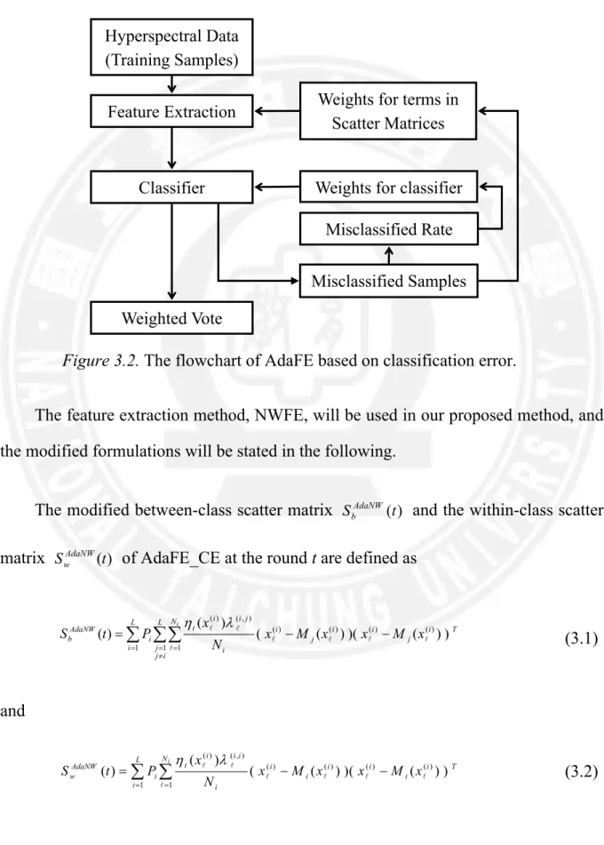
Figure 3.2 is the flowchart of adaptive feature extraction based on classification error (AdaFE_CE).
Figure 3.2. The flowchart of AdaFE based on classification error.
The feature extraction method, NWFE, will be used in our proposed method, and the modified formulations will be stated in the following.
The modified between-class scatter matrix SAdaNW(t)
b and the within-class scatter
matrix SAdaNW(t)
w of AdaFE_CE at the round t are defined as
T i j i L i L i j j N i j i i j i i t i AdaNW b x M x x M x N x P t S () i ( ) ( ( ))( () ( ())) 1 1 1 ) ( ) ( ) , ( ) (
(3.1) and T i i i L i N i i i i i i t i AdaNW w N x M x x M x x P t S ( ) i ( ) ( ( ))( () ( ())) 1 1 ) ( ) ( ) , ( ) ( (3.2) Feature Extraction Weighted Vote Misclassified Rate Weights for classifierWeights for terms in Scatter Matrices
Misclassified Samples Hyperspectral Data
(Training Samples)
where the scatter matrix weight ( ji,) is defined by
i N t i t j i t i j i j i x M x x M x 1 1 ) ( ) ( 1 ) ( ) ( ) , ( ) ) ( , dist( ) ) ( , dist( , (3.3) Nj k j k j i k i j x w x M 1 ) ( ) , ( ) ( ) ( , (3.4) and j N t j t i j k i j i k x x x x w 1 1 ) ( ) ( 1 ) ( ) ( ) , ( ) , dist( ) , dist( (3.5)denotes the weighted mean with respect to x(i)
in class j. On each round of AdaFE_CE, the weights
} , , 1 , , , 1 | ) ( { x() N i L i i t (3.6)
of each incorrectly classified training sample for defining modified scatter matrices are increased (or alternatively, the weights of each correctly classified training sample are decreased), so that the new extracted features focus more on those incorrectly classified training samples.
The algorithm of adaptive feature extraction based on classification error (AdaFE_CE) is described as following Table 3.1:
Table 3.1. The algorithm of adaptive feature extraction based on classification error.
1. Input:
(1) The training data x(i), 1, ,Ni,i 1, ,L
, and the test sample z.
(2) A classifier algorithm, (), with output ht() at the round t. (3) The reduced dimension, p.
2. Output: The label y of the test sample z by the ensemble.
A. Training Procedure: (1) Initialize weight: N i L N x i ) 1 , 1, , i, 1, , ( () 1 .
(2) Set the stop parameter q.
Do for t1 to…until εt -εt-1 q.
To build the classification including the linear transformation d p t
A
by applying AdaNWFE with SAdaNW(t)
b , SwAdaNW(t), and ) ( ) ( () T (i) t i t x A x h .
To estimate error for the training samples and estimate ( (), )
1 1 i t f x and t f2(t), where i u t t i t i t t i Z i x h i x h x x f / ) 10 ( ) ), ( ( )) ), ( ( 1 ( ) ( ) , ( () -) ( ) ( ) ( 1 .
Where Zt is a normalization constant,
i x h if i x h if i x h i t i t i t ) ( 0 ) ( 1 ) ), ( ( () ) ( ) ( ,
10] , 0 (
u , and f2 log(t/(1t)) is use to estimate classifier’s weights at the round t. B. Classification Procedure:
argmaxc 1,...,L 10t 1 t (ht(z),c) y .3.2.2 An Adaptive Feature Extraction with Reject Region
Figure 3.3. The flowchart of AdaFE with reject region.
In this section, we apply nonparametric weighted feature extraction to reduce the dimensionality of hyperspectral image, and train the classifier. In the classifier aspect,
Feature Extraction
Weighted Vote
Misclassified Rate Weights for classifier
Weights for terms in Scatter Matrices The samples of Reject Region Hyperspectral Data (Training Samples) Misclassified Samples Classifier
which come from the reject region into the next time process. Repeating iterations until convergence and then applying the weighted-vote way to combine classifiers. Figure 3.3 is the flowchart of adaptive feature extraction with reject region (AdaFE_RR).
The algorithm of adaptive feature extraction with reject region (AdaFE_RR) is described as following Table 3.2:
Table 3.2. The algorithm of adaptive feature extraction with reject region.
1. Input:
(1) The training data x(i), 1, ,Ni ,i 1, ,L
, and the test sample z. (2) A classifier algorithm, , with output () ht() at the round t. (3) The reduced dimension, p.
2. Output: The label y of the test sample z by the ensemble.
A. Training Procedure: (1) Initialize weight: N i L N xi ) 1 , 1, , i, 1, , ( () 1 .
(2) Set the stop parameter q.
Do for t1 to…until εt -εt-1 q.
To build the classification including the d p t
A linear transformation. - Applying adaptive nonparametric weighted feature extraction
- Creating the ( ()) ( T (i))
t i
t x A x
h .
To estimate RG(r) for the training samples and t.
- RG(r) {x(1),x(2), ,x([rN])}
- N x τ ε N i i t
1 ) ( ) ( -1 , where label true ) ( 0 label true ) ( 1 ) ( () ) ( ) ( i t i t i x h x h x τ . To estimate ( ) ( (), ) 1 ) ( 1 t i i t x f x . - i u t i i t t i Z r RG x r RG x x x f / (10) )) ( , ( ))) ( , ( 1 ( ) ( ) , ( -) ( ) ( ) ( ) ( 1 , where Zt is the normalization constants, ) ( 0 ) ( 1 )) ( , ( ) ( ) ( ) ( r RG x if r RG x if r RG x i i i , and u(0,10]. To estimate t f2(t), where f2 log(t/(1t)) is use to estimate the
weights for classifiers at the round t.
B. Classification Procedure:
argmaxc 1,...,L 10t 1 t (ht(z),c)
y .
3.2.3 An Adaptive Feature Extraction with Spatial Information
This processing includes two concepts for classifying hyperspectral image: (1) For avoiding the Hughes phenomenon, the feature extraction is the important for hyperspectral image classification. Hence, the feature space at the next round is varied at every round such that it suits for the misclassified samples at this round. The weights of the terms of the scatter matrices corresponding to the samples which are classified correctly at this round will be decreased in the next round. Otherwise, the weights will be increased for the samples which are misclassified. (2) Many studies (Bruzzone & Persello, 2009; Kuo, Chuang, Huang, & Hung, 2009) show that the performance of the
their classification performances at this round. The traditional hyperspectral image classification procedure is a special case of our proposed processing because it is the same to perform our proposed method one round without using spatial classifier. Fig. 3.4 shows the flowchart of adaptive feature extraction with spatial information (AdaFE_SI). Note that any type of classifier and feature extraction method can be used in our proposed procedure.
Figure 3.4. The flowchart of AdaFE with spatial information.
Feature Extraction
Weighted Vote
Misclassified Rate Weights for classifier Weights for Terms in
Scatter Matrices Misclassified Samples Hyperspectral Data (Training Samples) Spectral Classifier or Spatial Classifier
The algorithm of adaptive feature extraction with spatial information (AdaFE_SI) is described as following Table 3.3:
Table 3.3. The algorithm of adaptive feature extraction with spatial information.
1. Input:
(1) The training data x(i),1,,Ni,i1,,L.
(2) The test sample z.
(3) The classifier methods, spectral(), spatial()
with output at the round t. (4) The reduced dimension, p.
2. Output: The label y of the test sample z by the ensemble.
A. Training Procedure: (1) Initialize weight: N i L N x'i ) 1 , 1, , i, 1, , ( () 1 .
(2) Set the stop parameter q.
Do for t 1 to…until εt-εt-1 q.
To build the classification including the d p t
A linear transformation. Applying NWFE with SAda_NW(t)
b and Sw (t) Ada_NW . - i T j i L i L i j j N i j i i j i i t i Ada_NW b N x M x x M x x P t S ( ) i ( ) ( ( ))( () ( ())) 1 1 1 ) ( ) ( ) , ( ) ( . - i T i i L i N i i i i i i i t i Ada_NW x M x x M x N x P t S () i ( ) ( ( ))( () ( ())) 1 1 ) ( ) ( ) , ( ) ( w
. Creating the ( ())
T (i)
t spectral i t x A x h and ' ( ())
T (i)
t spatial i t x A x h . To estimate εt and ε't.- N x ε N i i t
1 ) ( ) ( -1 ' , where label true ) ( ' 0 label true ) ( ' 1 ) ( () ) ( ) ( i t i t i x h x h x . - otherwise if t t t 0 ' 1 . - errt tt (1t)'t. To estimate
t
i t f x err (), , 1 1 . -
i u
t t i t t u i t i t t i t t i Z i x h i x h i x h i x h x x f / 10 ) ), ( ' ( )) ), ( ' ( 1 ( ) 1 ( 10 ) ), ( ( )) ), ( ( 1 ( ) ( ) , ( -) ( ) ( -) ( ) ( ) ( ) ( 1 . Where Zt is the normalization constants, b a if b a if b a 0 1 ) , ( , and 10] , 0 ( u .
To estimate t f2
err , where f2 log(err/(1err)) is used to estimate classifier’s weights at the round t.B. Classification Procedure:
( ( ( ), ) (1 ) ( ' ( ), ))
max
arg 1,..., 101 h z c h z c
CHAPTER 4: DATASETS AND EXPERIMENTAL RESULTS
4.1 Hyperspectral Image Dataset and Experiments 4.1.1 Data Description
In this thesis, for investigating the influences of training sample sizes to the dimension, three distinct cases, Ni 20 N d (case 1), Ni 04 d N (case 2),
and d Ni 300N (case 3), will be discussed. Due to these sample size constraints, some of the classes in selected hyperspectral images for the experiment are used. The MultiSpec (Landgrebe, 2003) was used to select training and testing samples (100 testing samples per class) in our experiments which are the same method in (Benediktsson, Palmason, & Sveinsson, 2005), (Sebastiano & Gabriele, 2007), and (Landgrebe, 2003). At each experiment, ten training datasets and one testing dataset are randomly selected for estimating system parameters and computing the average accuracy of testing data of different algorithms respectively.
It is the Washington, DC Mall hyperspectral image (Landgrebe, 2003) as an urban site. The Washington, DC Mall image is a Hyperspectral Digital Imagery Collection Experiment airborne hyperspectral data flight line over the Washington, DC Mall. Two hundred and ten bands were collected in the 0.4–2.4 μm region of the visible and infrared spectrum. Some water-absorption channels are discarded, resulting in 191
channels. The dataset is available in the student CD-ROM of (Landgrebe, 2003). There are seven information classes in the Washington, DC data, roofs, roads, paths, grass, trees, water, and shadows, in the dataset.
4.1.2 Experimental Designs and Results
There is one dataset (Washington DC Mall Image) applied to compare the performances of non feature extraction (NonFE), NWFE, AdaFE_CE, AdaFE_RR, and AdaFE_SI methods in our experiments. In the AdaFE_CE and AdaFE_SI, the training error from 5-fold cross validation is used to renew the weights, u is set as 5. In the AdaFE_RR, the training error from 5-fold cross validation is used to renew the weights, u is set as 5, and r is set as 0.1. We create the classifiers under each different feature space, and finally combine them to turn into a strong classifier by weighted vote method.
Table 4.1. Number of pixels for each category
in the Washington DC Mall Image.
Category #(Pixels) 1 Roofs 3776 2 Roads 1982 3 Paths 737 4 Grass 2870 5 Trees 1430 6 Water 1156 7 Shadows 840 Total 12791
feature extraction (NonFE), NWFE, AdaFE_CE, AdaFE_RR, and AdaFE_SI. Table 4.2 displays the classification accuracies of testing data in cases 1, 2, and 3, respectively. Note that the highest accuracy of each dataset (in column) is highlighted in shadow cell. The brackets show the number of extracted features.
Table 4.2. The accuracy of Case 1, Case 2, and Case 3.
Case 1 Case 2 Case 3
Methods Classifier
Washington, DC Washington, DC Washington, DC
Gaussian N/A N/A 92.3 %
NonFE 3NN 84.3 % 87.5 % 94.2 % Gaussian 87.7 % (4) 92.0 % (4) 94.1 % (15) NWFE 3NN 88.9 % (4) 91.2 % (7) 95.1 % (8) Gaussian 89.2 % (11) 92.3 % (9) 94.1 % (13) AdaFE_CE 3NN 88.3 % (4) 91.1 % (5) 96.0 % (7) Gaussian 90.3 % (7) 93.7 % (15) 95.2 % (15) AdaFE_RR 3NN 89.2 % (4) 92.1 % (4) 95.5 % (8) Gaussian 93.1 % (8) 94.6 % (14) 95.0 % (14) AdaFE_SI 3NN 92.6 % (3) 94.3 % (7) 98.1 % (8)
The comparisons of mean accuracies between all algorithms using two different classifiers are displayed in Figures 4.2-4.7.
85% 87% 89% 91% 93% 95% NonFE NWFE AdaFE_CE AdaFE_RR AdaFE_SI NonFE 0% NWFE 87.70% AdaFE_CE 89.20% AdaFE_RR 90.30% AdaFE_SI 93.10% Gaussian (Case 1)
Figure 4.2. The accuracy of five methods with Gaussian classifier for hyperspectral
image classification in Case 1.
80% 83% 86% 89% 92% 95% NonFE NWFE AdaFE_CE AdaFE_RR AdaFE_SI NonFE 84.30% NWFE 88.90% AdaFE_CE 88.30% AdaFE_RR 89.20% AdaFE_SI 92.60% kNN (k=3, Case 1)
90% 91% 92% 93% 94% 95% NonFE NWFE AdaFE_CE AdaFE_RR AdaFE_SI NonFE 0% NWFE 92.00% AdaFE_CE 92.30% AdaFE_RR 93.70% AdaFE_SI 94.60% Gaussian (Case 2)
Figure 4.4. The accuracy of five methods with Gaussian classifier for hyperspectral
image classification in case 2.
85% 87% 89% 91% 93% 95% NonFE NWFE AdaFE_CE AdaFE_RR AdaFE_SI NonFE 87.50% NWFE 91.20% AdaFE_CE 91.10% AdaFE_RR 92.10% AdaFE_SI 94.30% kNN (k=3, Case 2)
Figure 4.5. The accuracy of five methods with kNN (k=3) classifier for hyperspectral
90% 91% 92% 93% 94% 95% 96% NonFE NWFE AdaFE_CE AdaFE_RR AdaFE_SI NonFE 92.30% NWFE 94.10% AdaFE_CE 94.10% AdaFE_RR 95.20% AdaFE_SI 95.00% Gaussian (Case 3)
Figure 4.6. The accuracy of five methods with Gaussian classifier for hyperspectral
image classification in case 3.
92% 93% 94% 95% 96% 97% 98% 99% NonFE NWFE AdaFE_CE AdaFE_RR AdaFE_SI NonFE 94.20% NWFE 95.10% AdaFE_CE 96.00% AdaFE_RR 95.50% AdaFE_SI 98.10% kNN (k=3, Case 3)
From these Table and Figures, we have the following findings.
1. In the Washington, DC Mall dataset, the highest accuracies among all methods are 93.1 % (AdaFE_SI with Gaussian classifier), 94.6 % (AdaFE_SI with Gaussian classifier), and 98.1 % (AdaFE_SI with 3NN classifier) in case 1, 2, and 3, respectively.
2. The best classification result is 98.1 % which is using AdaFE_SI with kNN (k=3) classifier.
3. According to the accuracy rate from Table 4.2, AdaFE_RR and AdaFE_SI with two different classifiers are better than conventional methods.
We choose the well-known Washington, DC Mall image as the example and only some classified images are shown for comparison. The classification mechanisms under case 1, 2, and 3 (Ni =20, 40, and 300) and five methods, NonFE, NWFE,
AdaFE_CE, AdaFE_RR, and AdaFE_SI, are selected to generate the classified images. Figures 4.9-4.13 are the classification maps from five feature extraction conditions (NonFE, NWFE, AdaFE_CE, AdaFE_RR and AdaFE_SI) with Gaussian and kNN (k=3) classifiers. It can be observed form Figures 4.9-4.13 that our novel methods with Gaussian or kNN (k=3) classifier outperform NonFE and NWFE with Gaussian or
Figure 4.8. Washington DC Mall Image.
■
Grass■
Path■
Tree■
Water■
Roof■
Road ■Shadow(a) (c)
(b) (d)
■
Grass■
Path■
Tree■
Water■
Roof■
Road ■Shadow(a) (d)
(b) (e)
(c) (f)
Figures 4.10. (a)-(c) AdaFE_CE with Gaussian classifier in cases 1, 2, and 3. Figures 4.10. (d)-(f) AdaFE_RR with Gaussian classifier in cases 1, 2, and 3.
■
Grass■
Path■
Tree■
Water■
Roof■
Road ■Shadow(a) (d)
(b) (e)
■
Grass■
Path■
Tree■
Water■
Roof■
Road ■Shadow(a) (d)
(b) (e)
(c) (f)
Figures 4.12. (a)-(c) NWFE with kNN (k=3) classifier in cases 1, 2, and 3. Figures 4.12. (d)-(f) AdaFE_CI with kNN (k=3) classifier in cases 1, 2, and 3.
■
Grass■
Path■
Tree■
Water■
Roof■
Road ■Shadow(a) (d)
(b) (e)
4.2 Educational Measurement Dataset and and Experiments 4.2.1 Data Description
According to the results of Chapter 4.1.2, the proposed methods, adaptive feature extractions, have better performance than other conventional methods. For evaluating student’s learning profile and arranging suitable remedial instruction, educational tests are usually administrated. In this section, educational measurement dataset is analyzed by the proposed methods and other conventional methods.
Performances of two algorithms listed in Chapters 3.2.1-3.2.2 are compared by using adaptive testing simulation processes with Mathematics paper-based test data. The content of the test designed for the sixth grade students is about “Sector” related concepts (see Appendix A). In Figure 4.14, the experts’ structures of the unit for this test are developed by seven elementary school teachers and three researchers. These structures are different from usual concept maps but emphasis on the ordering of nodes. Additionally, every node can be assessed by an item. There are 21 items in this test and 828 subjects are collected in “Sector” tests.
Figure 4.14. Experts’ structure of “Sector” unit.
Finding the areas of compound sectors
Finding the areas of simple sectors
Definition of sector Finding the areas of circles
Drawing compound graphs