應用倍頻取樣相位偵測器之鎖相迴路設計

全文

(1)國立交通大學電子工程學系電子研究所碩士班碩士論文. 應用倍頻取樣相位偵測器之鎖相迴路設計. Phase-Locked Loop Design with Double Sampling Phase Detector. 研究生：黃國爵. Guo-Jue Huang. 指導教授：溫瓌岸. 博士. Dr. Kuei-Ann Wen. 共同指導：溫文燊. 博士. Dr. Wen-Shen Wuen. 中華民國九十七年六月.

(2) 應用倍頻取樣相位偵測器之鎖相迴路設計 Phase-Locked Loop Design with Double Sampling Phase Detector 研究生：黃國爵. Student. ： Guo-Jue Huang. 指導教授：溫瓌岸博士. Advisor. ： Dr. Kuei-Ann Wen. 共同指導：溫文燊博士. Co-Advisor. ： Dr. Wen-Shen Wuen. 國立交通大學電子工程學系電子研究所碩士班碩士論文. A Thesis Submitted to Department of Electronics Engineering & Institute of Electronics Electronics College of Electrical and Computer Engineering National Chiao Tung University in Partial Fulfillment of the Requirements for the Degree of Master In Electronic Engineering June 2008. 中華民國九十七年六月.

(3) 應用倍頻取樣相位偵測器之鎖相迴路設計. 學生：黃國爵. 指導教授: 溫瓌岸博士共同指導教授: 溫文燊博士. 國立交通大學電子工程學系. 電子研究所碩士班. 摘要本論文提出應用倍頻取樣相位偵測器之鎖相迴路設計。倍頻取樣相位偵測器藉由加倍鎖相迴路之迴路頻寬降低鎖定時間，亦使參考頻雜訊移往高頻來降低參考頻雜訊。在系統分析方面，建立了一鎖相迴路使用倍頻取樣相位偵測器之線性模型。在驗證降低鎖定時間與參考頻雜訊的抑制方面，建立了 Verilog-AMS 鎖相迴路使用倍頻取樣相位偵測器與一般相位偵測器之暫態模型。在電路設計方面，設計一鎖相迴路可操作在倍頻取樣相位偵測器或一般相位偵測器模式，輸出頻率切換在 2.88 兆赫茲與 2.304 兆赫茲。在模擬結果中，鎖相迴路之鎖定時間可以降低 50﹪在 30ppm 的輸出頻率精準度，參考頻雜訊降低 16dB 且被移往倍頻。. i.

(4) Phase-Locked Loop Design with Double Sampling Phase Detector Student：Guo-Jue Huang. Advisor : Dr. Kuei-Ann Wen Co-advisor : Dr. Wen-Shen Wuen. Department of Electronics Engineering Institute of Electronics National Chiao-Tung University. Abstract In this thesis, a charge-pump phase-locked loop (PLL) design with double sampling phase detector (DSPD) is proposed. By using the double sampling phase detector, the PLL loop bandwidth is doubled to obtain the fast settling time and meanwhile shift the reference spur to higher frequency to suppress the reference spur. For system analysis, a third-order charge-pump PLL with DSPD linear model is developed. Verilog-AMS charge-pump PLL timing models with DSPD and conventional phase detector (PD) are developed to verify the fast settling time and reference spur suppression. A 2.304 GHz/ 2.88GHz charge-pump PLL with two operation modes, DSPD mode and conventional PD mode, is designed. From the simulation results, the settling time is reduced 50% in 30ppm frequency accuracy and the reference spur is suppressed 16dB.. ii.

(5) 誌謝這本論文得以完成，首先非常感謝溫瓌岸教授讓我有機會進入 TWT 實驗室，並給予我們豐富的資源、良好的學習環境，以及論文寫作的大方向。感謝溫瓌岸教授與溫文燊教授給予細心與耐心的指導，讓我在研究的路上走得平順。並感謝各位口試委員們－高曜煌教授與郭建男教授提供的寶貴建議與指教。感謝實驗室的學長姐們的指導與照顧：哲生學長、文安學長、晧名學長、立協學長、漢健學長、昱瑞學長、閎仁學長、建龍學長、家岱學長、建毓學長、及世基學長等。學長姐們的幫助與指導讓我獲益良多。感謝實驗室的同學們－佳欣、磊中、謙若、士賢、柏麟、俊彥，兩年來在課業和日常生活上總是相互的扶持，一起高興、一起嬉笑、一起度過難關。同時也要感謝實驗室的助理們－苑佳、淑怡、慶宏、恩齊、智伶、宛君、嘉誠，幫忙實驗室裡大大小小的事，讓我們能更專心於研究工作。最後，我要感謝家人無怨無悔的付出與支持，感謝好友們給我的鼓勵，最後感謝關心我與幫助我的人，僅以此論文與我的家人及好友分享我的收穫與喜悅。. 黃國爵 2008 年 6 月. iii.

(6) Contents 摘要 .........................................................................i Abstract .................................................................ii 誌謝 .......................................................................iii Contents................................................................iv List of Figures ......................................................vi List of Tables .........................................................x Chapter 1 Introduction ........................................1 1.1 Motivation............................................................................ 1 1.2 Phase-Locked Loop............................................................. 2 1.3 Linear Phase-Locked Loop model..................................... 4 1.3.1 Stability Analysis .................................................................................5 1.3.2 Settling Time........................................................................................8 1.3.3 Reference Spur ....................................................................................9. 1.4 Thesis Organization .......................................................... 11. Chapter 2 Double Sampling Phase Detector....12 2.1 Double Sampling Technique ............................................ 12 2.1.1Settling time........................................................................................12 2.1.2Reference Spur ...................................................................................13. 2.2 Double Sampling Phase Detector Architecture .............. 14 2.2.1 Phase Difference Smaller Than π ....................................................15 2.2.2 Phase Difference Larger Than π......................................................16. 2.3 Linear PLL Model with DSPD......................................... 19 2.3.1 Stability Analysis ...............................................................................19 2.3.2 Settling Time......................................................................................22 2.3.3 Reference Spur ..................................................................................22 iv.

(7) Chapter 3 System design and Verilog-AMS PLL Timing Model Verification.................................24 3.1 Phase Locked Loop System Design ................................. 24 3.2 Verilog-AMS Timing Model............................................. 26 3.2.1 Phase Detector...................................................................................27 3.2.2 Voltage Control Oscillator................................................................28 3.2.3 Feedback Divider ..............................................................................28 3.2.4 CML divide-by-two...........................................................................29. 3.3 Vreilog-AMS Phase Locked Loop Simulation................ 29. Chapter 4 Circuit Design and Implementation Results..................................................................32 4.1 Circuit Design.................................................................... 32 4.1.1 Phase Detector...................................................................................32 4.1.2 Charge pump.....................................................................................35 4.1.3 Voltage control oscillator ..................................................................36 4.1.4 Divider–CML divide-by-two ............................................................39 4.1.5 Divider–Feedback divider ................................................................39. 4.2 Simulation.......................................................................... 41 4.2 Measurement ..................................................................... 43. Chapter 5 Conclusions and Future Works.......51 5.1 Conclusions........................................................................ 51 5.2 Future works ..................................................................... 52. Bibliography........................................................56 Appendix .............................................................57 Vita .......................................................................61. v.

(8) List of Figures Figure 1.1 The typical transceiver architecture............................................................2 Figure 1.2 Effect of reference spurs of LO signal .......................................................2 Figure 1.3 Phase-locked loop.......................................................................................3 Figure 1.4 Phase detector of the charge-pump phase-locked loop ..............................3 Figure 1.5 The two-mode PLL.....................................................................................4 Figure 1.6 Linear model of the charge-pump phase-locked loop ................................5 Figure 1.7 Linear model of the third order charge-pump phase-locked loop ..............5 Figure 1.8 Bode plot of the third order charge pump PLL transfer function ...............7 Figure 2.1 Illustration of the settling time (a) Without double sampling. (b) With double sampling ...........................................................................................................13 Figure 2.2 Illustration of the reference spur effect on the VCO output spectrum without double sampling technique and with double sampling technique ..................13 Figure 2.3 The DSPD replaces the conventional PD in the PLL to achieve double sampling technique ......................................................................................................14 Figure 2.4 The timing diagram of the signals in DSPD with two input signal (Ref and VCO_N) phase difference (θe) is smaller than π .......................................................17 Figure 2.5 The timing diagram of the signals in DSPD with two input signal (Ref and VCO_N) phase difference (θe = π +θ'e) is larger than π. .............................................17 Figure 2.6 The average current and phase difference characteristic of the conventional PD and the double sampling phase detector ................................................................18 Figure 2.7 The linear model of the DSPD PLL ...........................................................19 Figure 2.8 The illustration of the phase margin degradation of the DSPD PLL with the same loop filter design .................................................................................................20. vi.

(9) Figure 2.9 The illustration of the modify design of the loop filter for the phase margin compensation for DSPD PLL ......................................................................................21 Figure 3.1 The open loop transfer function magnitude and phase response for the loop filter of the conventional PD PLL (CONPD) and DSPD PLL (DSPD).......................26 Figure 3.2 Block diagram of the Verilog-AMS model of the PFD and the charge pump with the non-ideal effects Figure .................................................................................27 Figure 3.3 (a) The block diagram of the feedback divider model. (b) D-FF divider-by-two circuit ..................................................................................................28 Figure 3.4 Block diagram of the CML divide-by-two model ......................................29 Figure 3.5 Control voltage of the VCO for frequency jump from 2.45GHz to 2.56GHz. In the 30-ppm frequency accuracy, the DSPD PLL (DS_PD) is locked at 20usec (m1) and the conventional PD PLL (CON_PD) is locked at 40usec (m2)...........................30 Figure3.6 Output spectrum of the PLL with the double sampling phase detector and the conventional phase detector. (a) Reference spur is -79.09dBm at 2.58GHz (m1). (b) Reference is -82dBm at 2.6GHz (m2) .........................................................................31 Figure 4.1 Schematic of the PLL operates in the DSPD model with control circuit ...33 Figure 4.2 The schematic of the PLL operates in the conventional PD model with control circuit ...............................................................................................................33 Figure 4.3 PFD with an EN signal ...............................................................................34 Figure 4.4 Schematic of the charge pump ...................................................................35 Figure 4.5 LC-tank voltage control oscillator..............................................................36 Figure 4.6 VCO output waveforms..............................................................................37 Figure 4.7 VCO output spectrum.................................................................................37 Figure 4.8 VCO output phase noise .............................................................................38 Figure 4.9 Tuning range...............................................................................................38. vii.

(10) Figure 4.10 (a) Divide-by-two circuit (b) implementation of the latch in CMOS technologies .................................................................................................................39 Figure 4.11 (a) The feedback divider architecture .......................................................40 Figure 4.11 (b) Four cascade DFF divide-by-two achieve divider ratio 16.................40 Figure 4.11 (c) Dual divider ratio (÷4/÷5) divider.......................................................40 Figure 4.11 (d) DFF divide-by-two..............................................................................40 Figure 4.12 VCO control voltage.................................................................................41 Figure 4.13 Output spectrum of the PLL with the DSPD mode and the conventional PD mode. (a) Reference spur is -52dBm at 2.898GHz (m1). (b) Reference is -68dBm at 2.916GHz (m2) ........................................................................................................42 Figure 4.14 Layout view of PLL design 1 ...................................................................43 Figure 4.15 VCO testing setup.....................................................................................44 Figure 4.16 Output spectrum of the VCO....................................................................45 Figure 4.17 Phase noise of the VCO............................................................................45 Figure 4.18 Tuning range of the VCO .........................................................................46 Figure 4.19 DSPD testing setup...................................................................................47 Figure 4.20 Conventional PD mode.............................................................................47 Figure 4.21 Layout view of PLL design 2 ...................................................................48 Figure 4.22 Output spectrum of the VCO....................................................................49 Figure 4.23 Phase noise of the VCO............................................................................49 Figure 4.24 Tuning range of the VCO .........................................................................50 Figure 5.1 Over sampling phase detector ....................................................................52 Figure 5.2 OSPD (n=2) ................................................................................................53 Figure 5.3 The signals in the OSPD (n=2)...................................................................54 Figure 5.4 The average current and phase difference characteristic of the over. viii.

(11) sampling phase detector (n=2). ....................................................................................55 Figure A-1 PLL model with feedback delay time........................................................57 Figure A-2 PLL linear model with noise sources ........................................................58 Figure A-3 Phase noise simulation ..............................................................................60. ix.

(12) List of Tables Table 2.1 Phase margin degradation with different ratio of the pole and the zero. .....20 Table3.1 The summary of the loop parameter of the phase locked loop with conventional phase detector.........................................................................................24 Table3.2 The summary of the loop parameter of the phase locked loop with double sampling phase detector...............................................................................................25 Table 4.1 Control circuit truth table.............................................................................34 :. x.

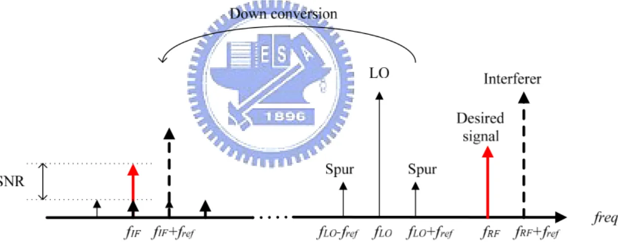
(13) Chapter 1 Introduction 1.1 Motivation In modern wireless communication systems, a frequency synthesizer in RF transceivers generate local oscillator (LO) signals for transmitter up conversion and receiver down conversion as shown in Figure 1.1. As multimode transceivers are integrated, the frequency synthesizer needs fast settling LO signals to provide seamless connectivity between different systems for mobile users. For example the requirement of the LO signal hopping time between WiMax and WiFi is limited in 10usec [1]. Frequency synthesizers are widely implemented by phase-locked loop technique and the settling time of the PLL-based frequency synthesizer is sensitive to the PLL loop bandwidth. PLLs with wide loop bandwidth can achieve fast settling time but the flowing large reference spur appearing at the upper and lower sideband will mix the interference (Interferer) signal to degrade the SNR of the desired signal, as shown in Figure 1.2. Hence for the PLL-based frequency synthesizer design, the requirement for fast settling and low reference spur is still a design issue. In this thesis, a double sampling technique is proposed to double the loop bandwidth to achieve fast settling and furthermore suppress the reference spur.. 1.

(14) Figure 1.1 The typical transceiver architecture.. Figure 1.2 Effect of reference spurs of LO signal. 1.2 Phase-Locked Loop A block diagram of a phase-locked loop system is shown in Figure 1.3. The elements of the system are a phase detector (PD), a loop filter, a voltage control oscillator (VCO) and a feedback divider. For conventional charge-pump phase-locked loop, the phase detector is implemented by a phase frequency detector (PFD) and a charge pump (ICP) as shown in Figure 1.4. The PFD samples the phase difference of. 2.

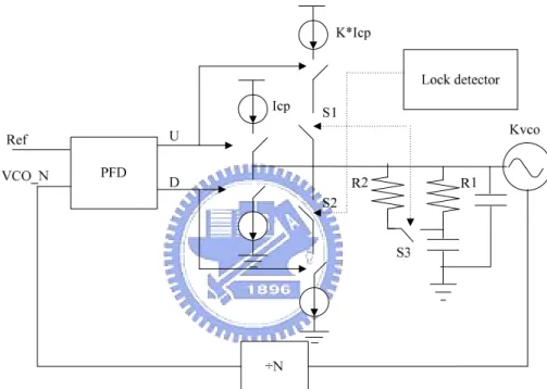
(15) the fref and fout_N, and produces sampling (Up/Down) signal pulse with pulse width proportional to the phase difference to control the charge pump switch. According to the sampling pulses the charge pump injects the average current in the loop filter every reference cycle. Hence, the phase difference of the conventional PD is sampled at the rate of the reference frequency.. Figure 1.3 Phase-locked loop.. Figure 1.4 Phase detector of the charge-pump phase-locked loop. A common solution for PLL design to achieve both fast settling and low reference spur is the variable loop bandwidth technique. In this technique, the PLL works with the wide loop bandwidth in tracking state and with the narrower loop bandwidth in locked state. Figure 1.5 shows the dual-mode PLL [2] to achieve the variable loop. 3.

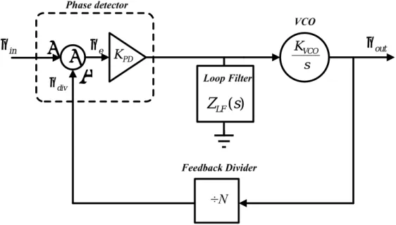
(16) bandwidth. In PLL tracking state, the switches (S1, S2) are shorted and more charges are injected in to the loop filter to reduce the settling time while the switches (S1, S2) are opened when in locked state. However the PLL switching between two different states needs a switch (S3) to change the loop filter and the parasitic capacitance in the switches (S1 ,S2 ,S3) create unwanted current injected in to the loop filter during the discontinuity switching between different loop bandwidths and may cause the PLL to lose lock.. Figure 1.5 The dual-mode PLL.. 1.3 Linear Phase-Locked Loop model A typical charge-pump phase-locked loop can be modeled as a linear system, as shown in Figure 1.6. The KPD is the phase detector gain and in the charge-pump PLL. The VCO is modeled as an integrator with a gain of KVCO (rad/s). The loop filter is modeled with a transfer function ZLF(s). The feedback divider is modeled as a constant N.. 4.

(17) θin. + + θe. −. θ div. KVCO s. K PD. θ out. Z LF ( s ). Figure 1.6 Linear model of the charge-pump phase-locked loop. 1.3.1 Stability Analysis In a third order charge-pump PLL with conventional PD, the loop filter is formed by one resistor and two capacitors as shown in Fig1.7. The loop filter creates one zero and one pole. The conventional PD gain is KCON_PD=ICP/2π, and ICP is the charge-pump current. θin. + + θ div. θe. −. K CON _ PD. Z LF ( s ). KVCO s. θ out. Figure 1.7 Linear model of the third order charge-pump phase-locked loop. 5.

(18) For analysis of the stability, the system phase margin is introduced. In the third order charge-pump PLL, the transfer function of the open-loop transfer function is K CON _ PD K VCO  1 + sτ z θ div = G (s) H (s) =  θe s 2C p Nτ z  1 + sτ p.   . (1.1). where G(s)=KCON_PDKVCOZLF(s)/s is the forward-loop transfer function, H(s)=1/N is the reverse-loop transfer function and τ z = RC z and τ p = R(C z || C p ) define the pole and zero. The frequency response of the gain of the open loop transfer function is − K CON _ PD K VCO  1 + jωτ z θ div |s = jω =  θe ω 2C p Nτ z  1 + jωτ p.   . (1.2). From equation (1.2), the unity gain of the open-loop transfer function can be derived as follow θ div θe. = 1 → ωu = ωBW _ CON =. K CON _ PD KVCO R b − 1. s = jωu. N. b. (1.3). where b=τz/τp. The unity gain is defined as the loop bandwidth ( ωBW _CON) of the PLL. The frequency response of the phase of the open-loop transfer function is φ (ω ) = −180o + tan −1 (ωτ z ) + tan −1 (ωτ p ). (1.4). From equation (1.4), the frequency corresponding to the maximum phase response can be defined from dφ (ω ) dω. =0. (1.5). then the relation between pole, zero and frequency corresponding to the maximum phase response can be expressed as ω = 1 τ zτ p. 6. (1.6).

(19) The phase margin (PM) is defined as PM = 180o + φ (ω = ωBW _ CON ) = tan −1 (ωBW _ CONτ z ) + tan −1 (ωBW _ CONτ p ). (1.7). From equation (1.6) and (1.7), to design the third order charge-pump PLL system with the maximum PM, the relation between the pole, zero and loop bandwidth must satisfy the equation (1.8). ωBW _ CON = 1 τ zτ p. (1.8). The maximum PM can be expressed as a function of the ratio between pole and zero, can be shown as  b −1  PM max = tan −1   2 b And the bode plot of the open loop transfer function is shown as Figure 1.8. GH ( s). ωz. ωu. ωp. ∠GH ( s ). Fig1.8 Bode plot of the third order charge pump PLL transfer function.. 7. (1.9).

(20) 1.3.2 Settling Time For the transient behavior of the third order charge-pump PLL, assuming the ratio between pole and zero is large, the third order charge-pump PLL will act like the behaviors of the second order charge-pump PLL. The settling time can be approximated as [3]. Tsettling.  tol  − ln  1− ς 2   f 2 − f1 . ≈ ςωn. (1.10). The initial frequency is f1 and the final frequency is f2. The final frequency accuracy is tol and the natural frequency and damping ratio are given by. ωn =. K PD KVCO NC z. K PD KVCO 1 ς = τz 2 NC z. (1.11). Equation (1.10) can be expressed as. Tsettling.  tol  −2 ln  1− ς 2   f 2 − f1  ≈ ωBW _ CON. ωBW _ CON =. K PD KVCO R N. (1.12). According to the equation (1.12), increasing the loop bandwidth can shorten the PLL settling time.. 8.

(21) 1.3.3 Reference Spur The periodic ripples on the control voltage of the VCO will modulate the VCO to generate the reference spur tone at the offset frequency fref from the carrier frequency. To estimate this effect, assume the VCO control voltage appears as a periodic function with a DC offset and expressed as V ( t ) = Vt + Am cos(ωref t ). (1.13). The VCO output can be modeled as Vout (t ) = Vo sin(ω freet + ∫ K vcoV ( t )dt ). (1.14). The magnitude of the reference spurs tone can be derived as follows Vout = Vo sin(ω freet + KVCO ∫ Vt dt + KVCO ∫ Am cos(ωref t )dt ) = Vo sin(ωout t +Vφ sin(ωref t )). (1.15). = Vo sin(ωout t ) cos(Vφ sin(ωref t )) + cos(ωout t ) sin(Vφ sin(ωref t ))  where ωout = ω free + KVCOVt and Vφ = Assume Vφ is small, i.e., Vφ = π. 2. KVCO Am ωref. , in equation (1.15). cos(Vφ sin(ωref t )) = 1. (1.16). and sin(Vφ sin(ω fref t )) ≈Vφ sin (ωref t ). (1.17). Equation (1.15) can be expressed as. Vout = Vo sin(ωout t ) + cos(ωout t )Vφ sin(ωref t ) . Vφ Vφ   = Vo sin(ωout t ) − sin(ωout − ωref ) + sin(ωout + ωref )  2 2  . 9. (1.18).

(22) From equation (1.18), the reference spur can be observed at the ωout ± ωref . The amplitude ratio between the reference spur and the carrier can be shown as. Areference spur Acarrier. =. ∆φ 1 KVCO Am = 2 2 ωref. (1.19). Equation (1.19) suggests that lower the VCO gain (Kvco) or the amplitude (Am) by reducing charge-pump current can suppress the reference spur but the PLL loop bandwidth will degrade. For both settling time and reference spur improvement, increasing the reference frequency is a way to extent the loop bandwidth and suppress the reference spur. In conventional PD the sampling rate is defined as the same as the reference frequency and the reference frequency is limited by the applications (channel bandwidth) and crystal. In this thesis, a phase detector doubling the phase difference sampling rate without changing the reference frequency is proposed to improve both settling time and reference spur performance.. 10.

(23) 1.4 Thesis Organization The thesis focuses on the design of phase-locked loop for fast settling and low reference spur. Chapter 2 presents a double sampling technique implemented by doubled sampling phase detector (DSPD). Then linear model of the DSPD is developed and the stability, settling time and reference spur analysis of the charge-pump PLL with DSPD is discussed. Chapter 3 introduces Verilog-AMS timing model for the proposed charge-pump PLL design. The timing model with non-idea effect is built to verify the settling time reduction and the reference spur suppression. The comparison of the proposed PLL with DSPD to that with conventional phase detector is performed through the Verilog-AMS timing models. In Chapter 4 presents the implementation of the charge-pump PLL with DSPD and conventional phase detector. The simulation and measurement results will be discussed. Chapter 5 comes out the conclusions and the future work.. 11.

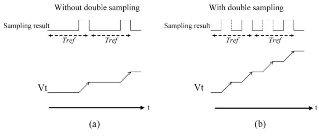
(24) Chapter 2 Double Sampling Phase Detector 2.1 Double Sampling Technique As discussion in Chapter 1, the settling time of the phase-locked loop is determined by the loop bandwidth of the PLL. According to the equation (1.12) and (1.19), increasing the reference frequency to raise the sampling rate of phase difference of the phase detector can improve the settling time and reference spur performance. In order to increase sampling rate of the phase detector without changing the reference frequency, the double sampling technique is proposed. 2.1.1Settling time The proposed double sampling technique for fast settling can be illustrated in Figure 2.1. Figure 2.1 (a) and Figure 2.1 (b) show the variation of the VCO control voltage (Vt) during the PLL frequency tracking without and with double sampling technique. In Figure 2.1 (a), the control voltage varies once in one reference cycle. On the other hand, using double sampling technique the control voltage varies twice in one reference cycle as shown in Figure 2.1(b). Comparing the Figure 2.1 (a) and Figure 2.1 (b), the variation of the control voltage with double sampling is more than that without double sampling in one reference cycle. Hence the settling time of the PLL can be reduced by employing double sampling technique.. 12.

(25) Fig 2.1 Illustration of the settling time (a) Without double sampling. (b) With double sampling.. 2.1.2Reference Spur Figure 2.2 illustrates the effect of the reference spur on the VCO output spectrum without and with double sampling technique.. Fig 2.2 Illustration of the reference spur effect on the VCO output spectrum without double sampling technique and with double sampling technique. As shown in Figure 2.2, using the double sampling technique the frequency of the periodic control voltage ripples can be doubled and the reference spur will be shift to two times of the reference frequency (2fref) away from the carrier. According to the equation (1.19), the amplitude ratio between the carrier and the reference spur is an inverse proportion to the sampling rate (fref) of the phase detector. Therefore, the. 13.

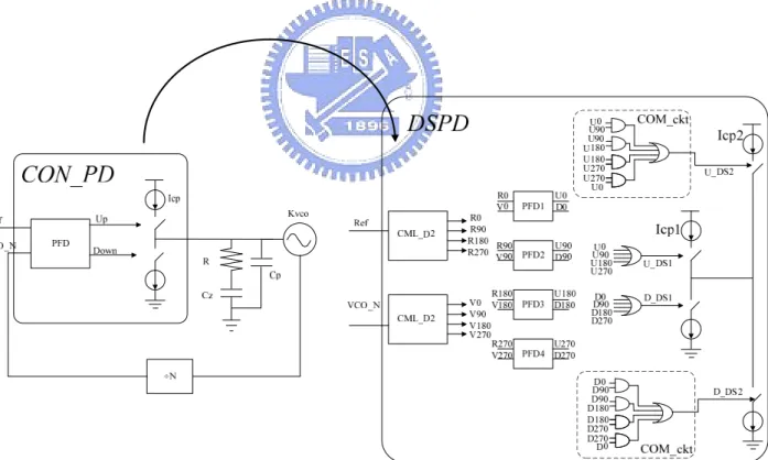
(26) reference spur could be suppressed as the reference spur shift far away from the carrier frequency.. 2.2 Double Sampling Phase Detector Architecture The PLL with double sampling technique to achieve fast settling and low reference spur is implemented by replacing the conventional phase detector (CON_PD) to the double sampling phase detector (DSPD) as shown in Figure 2.3. The DSPD is built with two common mode logic divide-by-two circuits (CML_D2), four PFDs, two charge pumps with the same current (Icp=Icp1=Icp2), two four-input OR gates and two compensation circuits (COM_ckt).. Figure 2.3 The DSPD replaces the conventional PD in the PLL to achieve double sampling technique.. 14.

(27) The conventional PD injects the average current proportional to the phase difference in the loop filter. The linear gain of the conventional PD (KCON_PD) architecture can be defined as I CON _ PD =. I CPθ e = K CON _ PDθ e 2π. (2.1). Comparing to the conventional PD, the DSPD injects two times of the average current proportional to the phase difference in the loop filter and the control voltage varies twice in one reference cycle. The linear gain of the DSPD architecture (KDSPD) can be defined by the detail DSPD circuit operation discussion according to the phase difference as follows.. 2.2.1 Phase Difference Smaller Than π Figure 2.4 shows the timing diagram of the signals in the DSPD with two input signals (Ref and VCO_N) with phase difference (θ e) is smaller than π. Each CML_D2 will produce four half-frequency and quadrature-phase output signals (R0~R270 and V0~V270). Then four phase frequency phase detectors sample the phase difference between the signals (R0/V0, R90/V90, R180/V180, R270/V270) of two CML-D2s in order to generate four sampling results (U0, U90, U180, U270). Each sampling result is proportional to the phase difference θ e. The OR gate combines the U0, U90, U180 and U270 to create one signal pulse, U_DS1 whose total pulse width is two times of the phase difference θe in one reference cycle. The output signal of the COM_ckt (U_DS2) will be always at low voltage in this region. Then the charge pump1 (Icp1) will be turned on twice in one reference cycle and the charge pump2 (Icp2) will always be turned off. The linear gain of DSPD in this region can be defined from the average current injected in the loop filter in one reference cycle. 15.

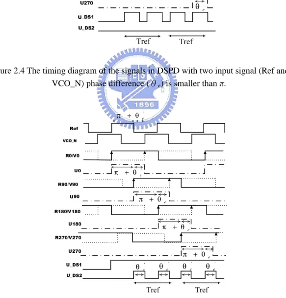
(28) I DSPD =. I CP1 (2θ e ) = K DSPDθ e 2π. for θ e < π. (2.2). Because the charge pumps in DSPD are designed to be the same as the charge pump in the conventional PD. Equation (2.2) can be expressed as:. I DSPD = K DSPDθ e = 2 K CON _ PDθ e. for θ e < π. (2.3). 2.2.2 Phase Difference Larger Than π Figure 2.5 shows the timing diagram of the signals in DSPD with two input signals (Ref and VCO_N) with phase difference (θe = π +θ'e) is larger than π. As discussed in previous section, the OR gate will create the U_DS1 signal whose pulse width is 2π. In addition, the COM_ckt will combine the (U0~U270) to create a signal pulse U_DS2 whose pulse width is proportional to θ'e. Therefore the charge pump1 will be always turned on and the charge pump2 will be turned on twice in one reference cycle. The average current injected in the loop filter in one reference cycle can be given as. I DSPD. I CP1 (2π ) + I CP 2 (2θ e' ) = 2π. (2.4). Because of the same charge pump current (Icp=Icp1=Icp2). The linear gain of the DSPD can be defined from. I CP1 (2π ) + I CP 2 (2θ e' ) 2 I CP (π + θ e' ) I DSPD = = = K DSPDθ e = 2 K CON _ PDθ e (2.5) 2π 2π for θ e > π. 16.

(29) θ. e. θ. e. θ. e. θ. e. θ. e. Figure 2.4 The timing diagram of the signals in DSPD with two input signal (Ref and VCO_N) phase difference (θe) is smaller than π. π + θ. π + θ. ' e. ' e. π + θ. ' e. π + θ. ' e. π + θ. θ. ' e. θ. ' e. θ. ' e. ' e. θ. ' e. Figure 2.5 The timing diagram of the signals in DSPD with two input signal (Ref and VCO_N) phase difference (θe = π +θ'e) is larger than π.. 17.

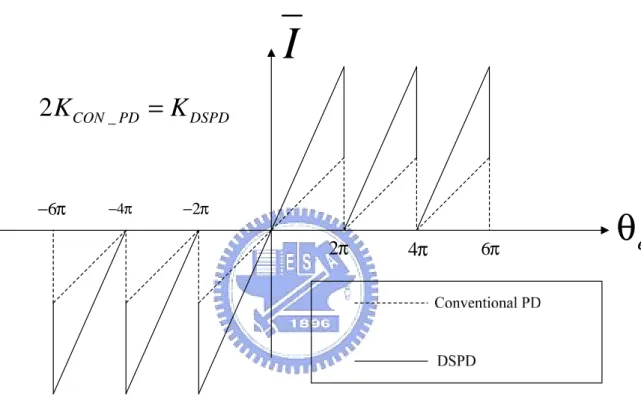
(30) As the discussion, the linear gain of the double sampling phase detector can be defined from equation (2.3) and (2.5). The Figure 2.6 shows the average current and phase difference characteristic of the conventional PD and the double sampling phase detector. Comparing to the conventional PD, the linear gain of the double sampling phase detector is doubled.. I 2 K CON _ PD = K DSPD. −6π. −4π. −2π. 2π. 4π. 6π. Figure 2.6 The average current and phase difference characteristic of the conventional PD and the double sampling phase detector.. 18. θe.

(31) 2.3 Linear PLL Model with DSPD The linear gain of the double sampling phase detector is doubled compared to the conventional PD. According to the equation (1.3), the loop bandwidth of the PLL with DSPD can be expressed as. ωBW _ DS =. 2 K CON _ PD KVCO R b K CON _ PD KVCO R b K DSPD KVCO R b = = N b −1 N b −1 N /2 b −1. (2.6). Therefore the linear model of the DSPD PLL can be regarded as the linear model of the conventional PD PLL using the half feedback divider ratio (N/2) with double reference frequency as shown in Figure 2.7.. θin. + + θ div. Z LF ( s ). θe. KVCO s. −. θ out. Figure 2.7 The linear model of the DSPD PLL.. 2.3.1 Stability Analysis As describe in Chapter 1, the phase margin of the third order charge-pump PLL can be designed by adjust the relation between loop filter and the loop bandwidth. For the same loop filter design, the PLL with DSPD will degrade the phase margin. 19.

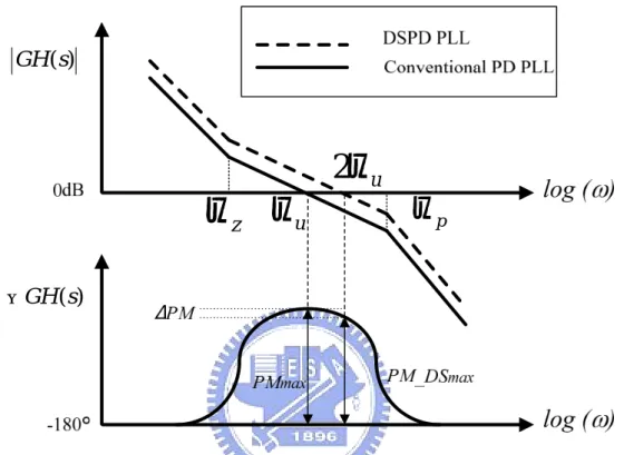
(32) because of the increase of loop bandwidth. The illustration of the phase margin degradation can be shown in Figure 2.8 and subsequently Table 2.1shows the phase margin degradation with different ratio of the pole and zero.. GH ( s ). 2ωu. ω z ωu. ωp. ∠GH ( s ). Figure 2.8 The illustration of the phase margin degradation of the DSPD PLL with the same loop filter design.. Table 2.1 The phase margin degradation with different ratio of the pole and the zero. b. PM_CON PM_DS ΔPM. 2.04. 20°. 18°. 2°. 3.00. 30°. 27.5°. 2.5°. 4.59. 40°. 36.6°. 3.4°. 5.82. 45°. 41.2°. 3.8°. 7.55. 50°. 45.8°. 4.2°. 10.06. 55°. 50.7°. 4.3°. 13.93. 60°. 55.6°. 4.4°. 32.16. 70°. 66.1°. 3.9°. 130.64. 80°. 77.7°. 2.3°. 20.

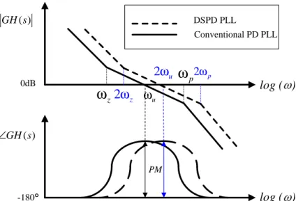
(33) To compensate the degradation of the phase margin, the modified loop filter design is proposed. In the conventional PD PLL, the maximum phase margin design satisfied the condition. ωBW _ CON = 1 τ zτ p = ω zω p. ωBW _ CON =. K CON _ PD KVCO R b N b −1. (2.7). The maximum phase margin of the system can be given as  b −1  PM max = tan −1   2 b. (2.8). For DSPD PLL, the loop bandwidth is doubled, ωBW _ DS = 2ωBW _ CON .. (2.9). In order to achieve the maximum phase margin design, double the frequency of the pole and the zero can still satisfy equation (2.7). 2ωBW _ CON = ωBW _ DSPD = (2ω z )(2ω p ). (2.8). According equation (2.8), since the simultaneous double of the frequency of the pole and the zero, b is the same and the phase margin can be remained maximum phase margin. The illustration of the loop filter design with phase margin compensation for DSPD PLL is shown in Figure 2.9.. GH ( s ). DSPD PLL Conventional PD PLL. 0dB. 2ωu ω p2ω p. ω z 2ω z ωu. log ( ). ∠GH ( s ) PM. log ( ). -180°. Figure 2.9 The illustration of the modify design of the loop filter for the phase margin compensation for DSPD PLL.. 21.

(34) 2.3.2 Settling Time The approximated settling time of the conventional PD PLL can be given as. Tsettling _ conventional _ PD.  tol  −2 ln  1− ς 2   f 2 − f1  ≈ ωBW _ CON. (2.10). For the DSPD PLL, the loop bandwidth is doubled therefore the settling time can be reduced by using the double sampling phase detector.. 2.3.3 Reference Spur For the conventional PD PLL the amplitude ratio between the reference spur and the carrier can be calculated by the approximation equation as  Aspur  1 KVCO Am =    Acarrier CON _ PD 2 ωref. (2.11). which Am and ωref are the amplitude and the frequency of the periodic ripples on the VCO control voltage (the sampling rate of the phase detector). The periodic ripples is due to the non-ideal effects of the phase detector such as mismatch of the charge pump, the leakage current from the control voltage and the timing error of the phase detector. AssumeΔI represents the total current due to the non-ideal effects injected in to the loop filter. The amplitude of the control voltage ripples can be expressed as Am = ∆I × R. (2.12). R is the resistance in the loop filter. Then equation (2.11) can be reformulated as equation (2.13) which is related to the loop bandwidth.  Aspur  1 ωBW _ CON ∆I = N   I CP  Acarrier CON _ PD 2 ωref. 22. (2.13).

(35) The loop bandwidth of the DSPD PLL is doubled and the linear model of the DSPD PLL can be regarded as the conventional PD PLL using half divider ratio (N/2) with double reference frequency (2ωref). Because of the periodic ripples due to the non-ideal effects of the phase effect occur when the PLL is in the lock state, as described in previous section, the charge pump2 is turned off and only the charge pump1 is operated. Then the non-ideal current of the DSPD PLL can be assumed the same as that of the conventional PD PLL. The approximation equation of the ratio between the reference spur and the carrier can be expressed as  Aspur  1 ωBW _ DSPD ∆I N 1 2ωBW _ CON ∆I N = =   I CP 2  Acarrier  DSPD 2 2ωref I CP 2 2 2ωref. (2.14). Comparing the equation (2.13) and (2.14), the reference spur can be suppressed about 6.02 dB by using double sampling phase detector even the loop bandwidth is doubled.. 23.

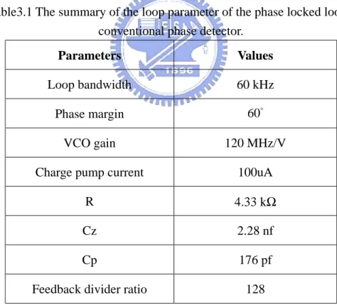
(36) Chapter 3 System design and Verilog-AMS PLL Timing Model Verification 3.1 Phase Locked Loop System Design Table 3.1 summarizes the loop parameter of the phase locked loop with the conventional phase detector. The VCO gain is 120 (MHz/V). The charge pump current is 100 uA. The feedback divider ratio is 128. In this work, the loop bandwidth and phase margin are chosen to be 60 kHz and 60°. Then the value of the components in the loop filter can be designed as R=4.33 kΩ, Cz= 2.28 nf, Cp= 176 pf.. Table3.1 The summary of the loop parameter of the phase locked loop with conventional phase detector. Parameters. Values. Loop bandwidth. 60 kHz. Phase margin. 60°. VCO gain. 120 MHz/V. Charge pump current. 100uA. R. 4.33 kΩ. Cz. 2.28 nf. Cp. 176 pf. Feedback divider ratio. 128. 24.

(37) The PLL using the double sampling phase detector needs to modify the loop filter design to compensate the phase margin degradation. According to the proposed loop filter modification in Chapter 2. Doubling the frequency of the pole and zero can remain the same maximum phase margin. Table 3.1 summarizes the loop parameters of the phase locked loop with the double sampling phase detector. As introduced in Chapter 2, the DSPD PLL can be regarded as conventional PD PLL with half divider ratio. The feedback divider ratio is 64. The charge pump current is 100 uA. The VCO gain is 120 (MHz/V) .Comparing to the conventional PD PLL, the loop bandwidth can achieve 120 kHz and phase margin remains 60°.. Table3.2 The summary of the loop parameter of the phase locked loop with double sampling phase detector. Parameters. Values. Loop bandwidth. 120 kHz. Phase margin. 60°. VCO gain. 120 MHz/V. Charge pump current. 100uA. R. 4.33 kΩ. Cz. 1.14 nf. Cp. 88 pf. Feedback divider ratio. 64. Figure 3.1 shows the magnitude and phase response of the open loop transfer function for the conventional PD PLL with the loop filter design in Table 3.1 and the DSPD PLL with the compensational loop filter design in Table 3.2.. 25.

(38) Figure 3.1 The open loop transfer function magnitude and phase response for the loop filter of the conventional PD PLL (CONPD) and DSPD PLL (DSPD).. 3.2 Verilog-AMS Timing Model To verify that the phase locked loop with double sampling phase detector can achieve fast settling and suppress the reference spur, a Verilog-AMS PLL timing model is developed. Verilog-AMS is a model language for Mixed-Mode system to describe the digital and analog circuits. For example the reference spur is generated by the non-ideal effects of the phase detector in time domain, the information then is transferred to the analogical quantity in the control voltage of the VCO. Therefore the Verilog-AMS PLL timing model with the phase detector non-ideal effects can be easily and efficiently described to illustrate the reference spur and transient behavior of the phase-locked loop.. 26.

(39) 3.2.1 Phase Detector The conventional phase detector in charge-pump PLL is implemented by the phase frequency detector and the charge pump. The non-ideal effects of the phase detector will create the reference spur due to the leakage current from the control voltage, the charge pump current mismatch and the Up/Down signals timing skew effect [4]. The block diagram of the Verilog-AMS model of the PFD and the charge pump with the non-ideal effects can be shown in Figure 3.2. The leakage current from the control voltage is modeled as a current source (Ileakage). The charge pump mismatch can be modeled with two current sources with different current Iup and Idown. The signals (Up/Down) to control the switch of the charge pump with a delay block (Tu, Td) for modeling the skew effect.. Figure 3.2 The block diagram of the Verilog-AMS model of the PFD and the charge pump with the non-ideal effects.. 27.

(40) 3.2.2 Voltage Control Oscillator The voltage control oscillator is modeled as a mathematical model that generates a periodic output whose frequency is a linear function of the control voltage, Vt. ωout = ω free + KVCOVt. (3.1). The ωfree and Kvco are the free running frequency and the gain of the VCO. Since the phase is the integral of the frequency with respect to time, the VCO output can be modeled as a sinusoidal function: Vout (t ) = A cos(ω freet + KVCO ∫ Vt dt ) t. −∞. (3.2). 3.2.3 Feedback Divider The feedback divider employs 7 stages divide-by-two to achieve the feedback divider ratio, 128, as shown in Fig 3.3(a). Each divider-by-two is implemented by the D-FF as shown in Figure 3.2(b).. Figure 3.3 (a) The block diagram of the feedback divider model. (b) D-FF divider-by-two circuit. 28.

(41) 3.2.4 CML divide-by-two The CML divide-by-two circuit can be modeled as two latches as shown in Figure 3.4. The divider-by-two circuit provides quadrature-phase outputs to implement the double sampling phase detector.. D. Q. I+. D. Latch1 clk. Q. Q+. Latch2 QB. I-. Qclk. QB. Vin. Figure 3.4 The block diagram of the CML divide-by-two model.. 3.3 Vreilog-AMS Phase Locked Loop Simulation The Verilog-AMS PLL model with conventional phase detector and double sampling phase detector is developed. For the conventional PD, set the delay block in PFD ( Td=0.1nsec, Tu=0.1nsec, Td=0.2nsec ) to model the skew effect. The charge current (Iup=100uA) and discharge current (Idown=90uA) to model the charge pump with 10% mismatch. The leakage current is 100nA. For DSPD, the delay block of the PFDs are settled the same as the PFD in the conventional PD. In addition the mismatch between charge current and discharge current of the two charge pumps in the DSPD are also considered the same as the charge pump in the conventional PD. Because of the DSPD has two charge pumps, the leakage current is settled as 200nA. In addition to the different phase detector, the PLL with conventional PD uses the loop filter design in Table 3.1 and the PLL with DSPD uses the loop filter design in. 29.

(42) Table 3.2 to eliminate the phase margin degradation. The VCOs and feedback dividers in two PLLs are the same. The free running frequency is 2.45 GHz and the VCO gain is 120 MHz. The reference frequency is 20MHz and the feedback divider ratio is 128, therefore the output frequency will be locked at 2.56 GHz. Figure 3.5 shows the control voltages of the VCO in the proposed Verilog-AMS PLL model with the conventional PD and DSPD as the frequency jump from 2.45GHz to 2.56GHz. The reduction of the settling time is 50% in the 30-ppm. Control voltage [V]. frequency accuracy.. 1.4 1.2 1.0 0.8 0.6 0.4 0.2 0.0 0. 10. 20. 30. 40. 50. time [usec]. Figure 3.5 Control voltage of the VCO for frequency jump from 2.45GHz to 2.56GHz. In the 30-ppm frequency accuracy, the DSPD PLL (DS_PD) is locked at 20usec (m1) and the conventional PD PLL (CON_PD) is locked at 40usec (m2).. 30.

(43) 0 m1. -50 -100 -150 -200. 2.61. 2.60. 2.59. 2.58. 2.57. 2.56. 2.55. 2.54. 2.53. 2.52. 2.51. VCO output spectrum [dBm]. 50. Freq [GHz]. 50 0 -50. m2. -100 -150 -200 2.61. 2.60. 2.59. 2.58. 2.57. 2.56. 2.55. 2.54. 2.53. 2.52. 2.51. VCO output spectrum [dBm]. (a). Freq [GHz] (b) Figure3.6 Output spectrum of the PLL with the double sampling phase detector and the conventional phase detector. (a) Reference spur is -79.09dBm at 2.58GHz (m1). (b) Reference is -82dBm at 2.6GHz (m2) Figure 3.6 shows the output spectra of the two Verilog-AMS PLL models with different phase detectors. The reference spur of the proposed PLL with double sampling phase detector is moved to two times of reference frequency from the carrier and is suppressed 5.9 dB more. DS_PD and CON_PD represent the PLL with double sampling phase detector and the conventional phase detector, respectively.. 31.

(44) Chapter 4 Circuit Design and Implementation Results 4.1 Circuit Design The reference spur suppression and the fast settling for the double sampling technique were verified by the linear model analysis and Verilog-AMS behavior model simulation in the previous chapters. In order to verify the performance improvement in real circuit, the process variation must be concerned. The PLL implementation must include both DSPD and conventional PD with the same VCO, feedback divider and the same quantity of the non-ideal effects of the phase detector. Figure 4.1 and Figure 4.2 show two digital signals, Vswitch and VPFD, to control the PLL for two operation modes, DSPD and conventional PD. The loop filter is off chip for different modes.. 4.1.1 Phase Detector Figure 4.1 shows schematic of the PLL operates in DSPD mode. The Vswitch controls the outputs of the 2-to-1 MUXs and the VPFD1 and VPFD234 control the PFDs. For the DSPD mode, first the Vswitch selects the outputs of MUXs (R0 and V0) to be output of the CML divide-by-two, then VPFD1 and VPFD234 the will turn on all the PFDs. Figure 4.2 shows the control signals control the PLL with the DSPD architecture but operates like the conventional PD. First the Vswitch selects the outputs of MUXs (R0 and V0) to be the signals Ref and VCO_N and only PFD1 is turned on. In this mode, the charge pump1 is operated and the charge pump2 is off. The PLL will operate in the conventional PD mode.. 32.

(45) VPFD Control circuit. VPFD1 VPFD234. Vswitch Vswitch 0 2-1 R0 1 Mux Ref. CML_D2. R90 R180 R270. CML_D2. PFD1. U0 D0. COM_ckt. Icp2 U_DS2. EN. Icp1. VPFD1 Vswitch 0 2-1 V0 1 Mux. VCO_N. R0 V0. U0 U90 U90 U180 U180 U270 U270 U0. V90 V180 V270. R90 V90 PFD2. U90 D90. EN. VPFD234 R180 U180 V180 PFD3 D180 EN. U0 U90 U180 U270 D0 D90 D180 D270. U_DS1. Off chip. VCO. R D_DS1. VPFD234 U270 R270 V270 PFD4 D270 EN. VPFD234. D0 D90 D90 D180 D180 D270 D270 D0. D_DS2. COM_ckt. ÷N. Figure 4.1 The schematic of the PLL operates in the DSPD model with control circuit. VPFD Control circuit. VPFD1 VPFD234. Vswitch Vswitch 0 2-1 R0 1 Mux Ref CML_D2. R90 R180 R270 Vswitch. R0 V0. PFD1. U0 D0. VCO_N CML_D2. V90 V180 V270. COM_ckt. Icp2 U_DS2. EN. Icp1. VPFD1 R90 V90 PFD2. U90 D90. EN. 0 2-1 V0 1 Mux. U0 U90 U90 U180 U180 U270 U270 U0. VPFD234 R180 U180 V180 PFD3 D180 EN. VPFD234 U270 R270 V270 PFD4 D270. U0 U90 U180 U270 D0 D90 D180 D270. U_DS1. Off chip. R D_DS1. EN. VPFD234. D0 D90 D90 D180 D180 D270 D270 D0. D_DS2. COM_ckt. ÷N. Figure 4.2 The schematic of the PLL operates in the conventional PD model with control circuit.. 33. VCO.

(46) The control circuit is designed according to the truth table as shown in Table 4.1. The OFF mode is defined as the PFDs are all turned off before the Vswitch is defined. To control the PFDs, the outputs signals of the control circuit VPFD1 and VPFD234 can be defined as the Boolean functions: VPFD1 = VPFD VPFD 234 = VPFDVswitch Table 4.1 Control circuit truth table. Input. mode. Output. Vswitch. VPFD. VPFD1. VPFD234. OFF. 0. 0. 0. 0. Conventional PD. 0. 1. 1. 0. OFF. 1. 0. 0. 0. DSPD. 1. 1. 1. 1. Because of the operation of the PFDs is controlled by the VPFD1 or the VPFD234, the PFDs are designed with a disable operation as shown in Figure 4.4. The EN signals of the PFDs are connected to the VPFD1 or VPFD234, so when the EN=0 then B=1 and the PFD is turned off otherwise when EN=1 then B=A the PFD is turned on.. EN=0. EN_ba =1. B=1 PFD turn off. EN=1. EN_ba =0. B=A PFD turn on. Figure 4.3 The PFD with an EN signal.. 34.

(47) 4.1.2 Charge pump The charge pump transfer the pulse of the phase detector to the charge injected in to the loop filter. The charge pump circuit is shown in Figure 4.5. The M1, M2, M5 is to generate the bias current. The current mirror M3, M4, M5, M6 is to generate the I2 is as same as the I1. The charge pump1 is composed by M10, M11, M12, M13 and the charge pump 2 is composed by M14, M15, M16, M17. In charge mode, the charge pump1 and the charge pump2, the M6, M7, M10, M11, M14 and M15 are designed to set I2=Iup1=Iup2. In discharge mode for the charge pump1 and the charge pump2, the M8, M9, M12, M13, M16 and M17 are to let I2=Idown1=Idown2.. Figure 4.4 The schematic of the charge pump.. 35.

(48) 4.1.3 Voltage control oscillator In this PLL design the VCO is implemented by the LC-tank voltage control oscillator because of the high frequency accuracy and low phase noise performance and it is shown in Figure 4.6. The NMOS M1 and M2 make up the cross-coupled pair to provide a negative resistance (Rn=-2/gm1,2) to compensate the loss of the LC tank. The NMOS M4 acts as a varactor, the capacitance (ΔC(Vtune)) between gate and drain can be control by the Vtune. The switch-capacitance (C1 and C2) are used to enlarge the tuning range and remain the small VCO gain at the same time [4]. The output frequency can be expressed as ωout =. 1. (. L CL + CL' + ∆C (Vtune ). ). CL' is related to the ON/OFF of the switch D1 and D0.. Figure 4.5 LC-tank voltage control oscillator.. 36.

(49) The VCO simulation results including the time domain VCO output waveform, VCO output spectrum, phase noise and tuning range are shown in Figure 4.6, Figure 4.7, Figure 4.8 and Figure 4.9, respectively. Figure 4.8 shows the phase noise at the one and two times reference frequency (18MHz and 36 MHz) offset from the carrier are -135.3dBc and -143dBc.. Figure 4.6 VCO output waveform. Figure 4.7 VCO output spectrum. 37.

(50) Phase noise [dBc]. Offset frequency [Hz] Figure 4.8 VCO output phase noise. Figure 4.9 Tuning range. 38.

(51) 4.1.4 Divider–CML divide-by-two The CML divide-by-two [5] is realized as two latches in a negative feedback loop as shown in Figure 4.11 (a). Figure 4.11 (b) is the latch circuit implemented in CMOS technology.. (a). Q. D ck. ckba. (b) Figure 4.10 (a) Divide-by-two circuit (b) implementation of the latch in CMOS technology.. 4.1.5 Divider–Feedback divider The block diagram of the feedback divider is designed as shown in Figure 4.11 (a). The divider ratio can be 128 or 160 with the control signal MC. The first stage of the feedback divider is implemented by four cascade DFF divide-by-two to achieve divider ratio 16 as shown in Figure 4.11 (b). The first two DFF dividers are implemented by TSPC divide-by-two [6] for high frequency operation and the last. 39.

(52) two stages are implemented by the CMOS logic. The second stage of the feedback divider is designed as a dual divider ratio (÷4/÷5) divider as shown in Figure 4.11 (c). The last stage of the feedback divider is implemented by the DFF as shown in Figure 4.11 (d).. Figure 4.11 (a) The feedback divider diagram.. Figure 4.11 (b) Four cascade DFF divide-by-two achieve divider ratio 16.. Figure 4.11 (c) Dual divider ratio (÷4/÷5) divider.. Figure 4.11 (d) DFF divide-by-two. 40.

(53) 4.2 Simulation The post layout simulation results of the PLL are shown in Figure 4.12 and Figure 4.13, including the control voltage of the VCO and the VCO output spectrum. DS_PD and CON_PD denote the PLL with double sampling mode and the conventional phase detector mode, respectively.. 1.8. DS_PD. VCO control voltage [V]. 1.6. 2.88 GHz. 1.4 1.2. CON_PD 2.304 GHz. 1.0 0.8 0.6 0.4 0.2 0. 5. 10. 15. 20. 25. 30 35. 40. 45. 50. 55. 60. 65. 70. 75 80. 85. 90. 95 100. Figure 4.12 VCO control voltage. The PLL locks to 2.88 GHz first then switch to 2.304 GHz at 30usec. From the post-simulation result, in the 30-ppm frequency accuracy the PLL with DSPD mode is locked at 42usec (m1) and the PLL with conventional PD mode is locked at 54usec. Hence the settling time is reduced 50% with the proposed DSPD technique.. 41.

(54) VCO Output Spectrum [dBm]. 10. -30. m1. -80. -130 2.826. 2.844. 2.862. 2.880. 2.898. 2.916. 2.934. Freq [GHz]. VCO Output Spectrum [dBm]. 10. -30. m2 -80. -130 2.826. 2.844. 2.862. 2.880. 2.898. 2.916. 2.934. Freq [GHz]. Figure 4.13 Output spectrum of the PLL with the DSPD mode and the conventional PD mode. (a) Reference spur is -52dBm at 2.898GHz (m1). (b) Reference is -68dBm at 2.916GHz (m2).. The reference spur of the PLL with DSPD mode is moved to two times of the reference frequency away from the carrier and is suppressed 16 dB. Comparing to the linear model analysis the reference spur can be suppressed more than 6.2 dB because of the suppression of the LC-tank.. 42.

(55) 4.2 Measurement PLL design 1 Figure 4.14 shows layout photo of the PLL design 1 using the PMOS LC-tank VCO. The PLL is fabricated in UMC CMOS 0.18um technology.. Figure 4.14 Layout view of PLL design 1.. 43.

(56) VCO measurement Figure 4.15 shows the testing setup for the phase noise and the spectrum measurement of the voltage control oscillator. It consists a spectrum analyzer, a power supply and two open drain matching network. One of the VCO outputs is terminated by a load having impedance of 50Ω and the other is connected to the spectrum analyzer.. Spectrum Analyzer. Power Supply. DUT. Figure 4.15 VCO testing setup. The measured output spectrum at 2.528 GHz is shown in Figure 4.16. The output power including the cable loss is -8.76dBm. Figure 4.17 shows the phase noise measurement result of the voltage control oscillator with the carrier frequency 2.528 GHz. The measured phase noise is -102.85 (dBc/Hz) at 1-MHz frequency offset.. 44.

(57) Figure 4.16 Output spectrum of the VCO. Figure 4.17 Phase noise of the VCO. 45.

(58) Output frequency [GHz]. 2.9. 2.6. 2.8 2.5 2.7 2.4. 2.6 2.5. 2.3. 2.4 2.2. 2.3 2.2. 2.1 0.0. 0.2. 0.4. 0.6. 0.8. 1.0. 1.2. 1.4. 1.6. 1.8. 2.0. 0.0. 0.2. 0.4. 0.6. 0.8. 1.0. 1.2. 1.4. 1.6. Figure 4.18 Tuning range of the VCO Comparing to the measurement and post-simulation of the tuning range results, the carrier frequency is degraded and the tuning range of the measurement is about 40 MHz/V and the post-simulation results is about 200 MHz/V. The performance degradation is caused by the parasitic capacitance.. DSPD measurement Figure 4.18 shows the testing setup for the DSPD. It consists a 2 MHz crystal, a power supply and a oscilloscope. The power supply provides not only VDD power but also the control signals Vswitch and VPFD to select the PLL operation mode. The crystal and delay block which is implemented by a RC circuit create two input signals with different phase (Ref and VCO_N). The oscilloscope can measure the outputs including the outputs of the MUXs, U_DS1, U_DS2, D_DS1 and D_DS2.. 46. 1.8.

(59) Figure 4.19 DSPD testing setup Figure 4.19 shows the measurement results for conventional PD mode (Vswitch=0 V and VPFD =1.8 V). The DSPD is operated in conventional PD mode by the control signal.. Ref VCO_N D_DS1 U_DS1. Figure 4.20 Conventional PD mode. For DSPD mode (Vswitch=1.8 V and VPFD =1.8 V), the control signal node Vswitch has a leakage current about 5mA and the DSPD mode can not operate correctly.. 47.

(60) PLL design 2 Figure 4.21 shows layout photo of the PLL design 2 using the NMOS LC-tank VCO. The PLL is fabricated in UMC CMOS 0.18um technology.. Figure 4.21 Layout view of PLL design 2.. VCO measurement The VCO testing setup is as same as that for the PLL design 1. The measured output spectrum is 2.336 GHz as shown in Figure 4.22. The output power including the cable loss is 4.9dBm. Figure 4.23 shows the phase noise measurement result of the voltage control oscillator with the carrier frequency 2.36 GHz. The measured phase noise is -84.23 (dBc/Hz) at 1-MHz frequency offset. The measurement and post-simulation results of the tuning range are shown in Figure 4.24, the measurement is about 60 MHz/V and the post-simulation is about 200 MHz/V. The performance degradation is caused by the parasitic capacitance.. 48.

(61) Figure 4.22 Output spectrum of the VCO. Figure 4.23 Phase noise of the VCO. 49.

(62) 3.0. Output frequency [GHz]. 2.8. 2.8. 2.6. 2.6 2.4. 2.4 2.2. 2.2 0.0. 0.2. 0.4. 0.6. 0.8. 1.0. 1.2. 1.4. 1.6. 1.8. 0.0. 0.2. 0.4. Figure 4.24 Tuning range of the VCO. 50. 0.6. 0.8. 1.0. 1.2. 1.4. 1.6. 1.8.

(63) Chapter 5 Conclusions and Future Works 5.1 Conclusions In this thesis, a novel PLL architecture with double sampling phase detector is proposed to achieve both fast settling time and low reference spur. Comparing with the conventional phase detector, the double sampling phase detector doubles the sampling rate of the phase detector without changing the reference source. The linear model of the third order charge-pump PLL with DSPD is developed. The linear gain of DSPD is doubled to achieve wider PLL loop bandwidth to reduce the settling time meanwhile the reference spur can be suppressed by the sampling rate of the phase detector is doubled. To compensate the phase margin degradation, the compensational loop filter design for PLL with DSPD is proposed. The PLL system with conventional PD and DSPD are designed and the Verilog-AMS PLL timing model with phase detector non-ideal effects is developed to verify the settling time and reference spur improvement. From the timing model simulation results, the settling time can be reduced 50% in 30-ppm frequency accuracy and the reference spur shifts to two times reference frequency from carrie.r In order to eliminate the process variation, a 2.304GHz/2.88GHz PLL with the conventional PD and DSPD operation modes is deigned. Simulation results show the settling time can be reduced 50 % in 30-ppm frequency accuracy and the reference spur can be shift to two times reference frequency from carrier and suppress 16 dB.. 51.

(64) 5.2 Future works Since increasing the sampling rate of the phase detector can improve both settling time and reference spur performance, the DSPD architecture can be modified to achieve over sampling phase detector. The over sampling ideal is to increase the phase detector sampling rate without changing the reference source. The architecture for over sampling phase detector (OSPD) can be shown in Figure 5.1. To achieve over sampling, the delay blocks (Td = Tref/(n+1)) can be employed to generate multiphase of Ref and VCO_N signals, and n PFDs generate the phase difference from the multiphase outputs (R0/V0, R1/V1…Rn/Vn). Then the n-input OR gate combines the sampling results to be one output signal (U1/D1). The COM_ckt will generate signals (U2/D2) to control the charge pump2.. Figure 5.1 Over sampling phase detector.. 52.

(65) The limitation of the OSPD is the detection region of the phase detector will be narrow as the n is increase. For example OSPD for n=2, the circuit is shown in Figure 5.2.. OSPD (n=2). 1×Td. PFD0 D0. Icp1 U1 PFD1 D1 U2 PFD2. V0. 2×Td. U_2. U0. R2. 1×Td. Icp2. U2 U0. R1. 2×Td. VCO_N. COM_ckt. U0 U1 U1 U2. R0. Ref. U0 U1 U2. U_1. D0 D1 D2. D_1. D2. V1 D0 D1 D1 D2. V2. D_2. D2 D0. COM_ckt. Figure 5.2 OSPD (n=2) The linear gain can be defined from the signals time diagram in OSPD (n=2) as shown in Figure 5.3. Assume the charge pump current are the same. For the phase difference smaller than the 2π/3, the average current injected in the loop filter in one reference cycle can be given as I=. I CP1 (3θ e ) I CP (3θ e ) = 2π 2π. for. 2π. 3. < θe. (5.1). For 2π/3 < phase difference ( θ e = 2π + θ e' ) < 4π/3, the average current injected 3 in the loop filter in one reference cycle can be given as I CP1 (2π ) + I CP 2 (3θ e' ) 3( I= = 2π. 2π + θ ' ) I 3 e CP 2π. for 2π. 4. < θ e < 4π (5.2) 3. For 4π/3 < phase difference ( θ e = 4π + θ e' ) < 2π, the average current injected 3 in the loop filter in one reference cycle can be given as I=. I CP1 (2π ) + I CP 2 (2π ) 4π I CP = 2π 2π. 53. for. 4π. 3. < θ e < 2π. (5.3).

(66) Phase difference < 2π Td. 2π. 3. R0=Ref. 3. < Phase difference < 4π Td. 2π + θ ' 3 e. V0=VCO_N. U0 R1=Ref+Td R1=VCO_N+Td U1 R2=Ref+2Td R2=VCO_N+2Td U2. U_1 U_2 Tref. Tref. 4π. 3. < Phase difference < 2π Td. R0=Ref V0=VCO_N. 4π + θ ' 3 e. U0 R1=Ref+Td R1=VCO_N+Td U1 R2=Ref+2Td R2=VCO_N+2Td U2. U_1 U_2 Tref. Figure 5.3 The signals in the OSPD (n=2).. 54. 3.

(67) The average current and phase difference characteristic of the OSPD (n=2) can be shown as Figure 5.4. The detection range of the OSPD (n=2) is -4π/3 < θ e < 4π/3. For more deep sampling technique, the logic circuit must be modified to extend the detection region. The process variation of the delay block will cause the phase noise performance degradation as discuss in reference [7]. In order to estimate the performance degradation due to the process variation more accuracy multiphase generator circuit is needed.. I. −2π. −4π. 3. −2π. 3. 2π. 3. 4π. 3. 2π. θe. Figure 5.4 The average current and phase difference characteristic of the OSPD (n=2).. 55.

(68) Bibliography [1] Meng-Ting Tsai, Ching-Yuan Yang, “A Fast-Locking Agile Frequency Synthesizer for MIMO Dual-mode WiFi/WiMAX Applications” Electronics, Circuits and Systems, 2007. ICECS 2007, pp.1384-1387, Dec. 2007. [2] H. Sato, K. Kato, and T. Sase, “A fast pull-in PLL IC using two-mode pull-in technique” Electron. Commun. Jpn ,pt. 2,vol. 75, no. 3, pp.41-50, 1992. [3] Dean Banerjee “PLL Performance, Simulation and Design, Fourth Edition”. [4] Tsung-Hsien Lin and William J.Kasier, “A 900MHz 2.5mA CMOS Frequency Synthesizer with an Automatic SC Tuning Loop” IEEE J.Solid-Seate Circuits, vol.36, pp.424-431, March. 2001. [5] B. Razavi, “RF Microelectronics” [6] S. Pellerano, S. Levantino, C. Samori, A.L. Lacaita “A 13.5-mW 5-GHz Frequency Synthesizer with Dynamic-Logic Frequency Divider” IEEE J.Solid-State Circuits, vol.39, pp378-383, FEBRUAY 2004 [7] T. C. Lee; W. L. Lee “A Spur Suppression Technique for Phase-Locked Frequency Synthesizers” IEEE ISSCC, pp. 2432 – 2441, 2006. [8] Bosco Leung “VLSI for Wireless Communication” [9] Dan FitzPatrick and Ira Miller “Analog Behavior Modeling with the Verilog-A Language” [10] B. Razavi, “Challenges in the design of frequency synthesizers for wireless applications” IEEE Custom Integrated Circuits Conference, pp.395-402, May 1997 [11] Woogeun Rhee, “Design of high-performance CMOS charge pumps in phase-locked loops” Circuits and Systems, 1999. ISCAS 1999. pp.545-548, May. 1999. [12] Keliu shu Edgar Sanchez-Sinencio, “CMOS PLL SYNTHERIZERS Analysis and Design”. 56.

(69) Appendix Feedback Delay Effect in PLL Figure A-1 (a) and Figure A-1 (b) show the PLL linear model with the feedback delay for different phase detector architectures. In Figure A-1 (a), the delay effect in the feedback path is modeled as e-sTD, TD is the delay time of feedback divider. In Figure A-2 (a), the delay effect in the feedback path is modeled as e-s(TD+TCML_D2) including the delay time of CML divider-by-two (TCML_D2). PFD and Charge Pump Loop Filter. θin. + + θe θ div. −. KVCO s. K PD. Loop Filter. DSPD. VCO. Z LF ( s ). θout. θin. R. + + θe θ div. Cp. −. VCO. Z LF ( s ) KVCO s. KCON_PD R Cp/2. Cz. Cz/2. Feedback Divider. Feedback Divider. e − sTD. ÷N. e. − s (TD +TCML _ D 2 ). (a). ÷N/2. (b). Figure A-1 PLL linear model with feedback delay time In real circuit, the signal delay degrades the system phase margin [12] and the can be shown as PM ' = PM − ωBW T. (A.1). ωBW and T are the PLL loop bandwidth and the delay time of the feedback divider. In Figure A-1, the phase margin degradation due to delay effect can be expressed as ' PM CON = PM CON − ωCON _ BW TD ' PM DSPD = PM DSPD − ωDSPD _ BW (TD + TCML _ D 2 ). (A.2). DSPD PLL doubles the PLL loop bandwidth and the modified loop filter design can remains the same phase margin (PMCON=PMDSPD). However, the phase margin is. 57. θ out.

(70) degraded by the additional delay time of the CML divide-by-two and can be expressed as ' ' − PM CON PM DSPD. =  PM CON − ωCON _ BW TD  −  PM CON − 2ωCON _ BW (TD + TCML _ D 2 ) . (A.3). = ωCON _ BW (TD + 2TCML _ D 2 ) According to feedback divider and CML_D2 circuit design in Chapter 5, the delay time of the feedback divider and CML divide-by-two are 0.2542nsec and 0.5nsec. The phase margin degradation is ' ' PM DSPD − PM CON = 2π × 60k × (0.2542n + 0.5n) ≈ 2.8 ×10−4 (rad / sec) = 0.0162° (A.4). The phase margin degradation due to the feedback delay is small and can be neglected.. Noise Consideration of PLL The transfer function from the noise sources to the output of the PLL can be obtained by the linear model as shown as Figure A-2.. θin. + + θe θ div. −. K PD. +. θVCO. Vn , R. I n ,CP. Z LF ( s ). +. KVCO s. +. θ out. Figure A-2 PLL linear model with noise sources. The transfer function from the input phase (θin) to the output phase (θout) can be expressed as following equation and is a low-pass function.. 58.

(71) K K PD Z LF ( s ) VCO θ out s = ( ) K Z s K θin 1 + PD LF VCO Ns. (A.5). Therefore, the phase noise of the reference is attenuated at large frequency offset. The transfer function from the VCO noise (θVCO) to the output phase can be expressed as the following equation and is a high-pass function. θ out 1 = K Z θVCO 1 + PD LF ( s ) KVCO Ns. (A.6). The far-offset phase noise of the PLL is dominated by the VCO phase noise. The transfer function from the charge pump noise (In,CP) to the output phase can be expressed as the following equation and is a low-pass function. K Z LF ( s ) VCO θ out s = K Z s ( I n ,CP 1 + PD LF ) KVCO Ns. (A.7). The charge pump noise can be represented as [12] I n ,CP = 2. ton 2I 4kT CP Tref Vod _ cp. (A.8). where the ton is the turn-on time of the charge pump and Vod_cp is the overdrive voltage (VGS-Vt) of the transistor in charge pump circuit as shown in Figure 4.4. In DSPD, the noise of the charge pump 2 can be neglected because of charge pump current noise is dependent to the turn-on time. The transfer function from the thermal noise of R (Vn,R) to the output phase can be expressed as the following equation and is a band-pass function. θ out Vn , R. KVCO s = K PD Z LF ( s ) KVCO 1+ Ns. (A.9). The phase noise simulations are performed in Advanced Design System (ADS). The. 59.

(72) simulation result is shown in Figure A-3 (a). Since the transfer function from VCO phase noise to output phase noise indicated in equation 4.22 is a high-pass characteristic. The far-offset phase noise of the PLL is dominated by VCO. The close-in offset phase noise of the PLL is dominated by the reference source. The phase noise reduction of the DSPD PLL comparing to the conventional PD PLL can be shown in Figure A-3 (b). The close-in offset phase noise can be reduced 6dB due to the loop bandwidth extension of the DSPD PLL. 100 VCO free running phase noise. Phase noise [dBc/Hz]. 50 0 CON. -50 DSPD. -100. Dominated by reference noise. -150. Dominated by VCO. -200 1. 1E1. 1E2. 1E3. 1E4. 1E5. 1E6. 1E7. 1E8. 1E6. 1E7. 1E8. Frequency [Hz] (a). Phase noise reduction (CON - DSPD) [dBc/Hz]. 8 6 4 2 0. -2 1. 1E1. 1E2. 1E3. 1E4. 1E5. Frequency [Hz] (b). Figure A-3 Phase noise simulation.. 60.

(73) Vita 姓名 : 黃國爵性別 : 男出生地 : 桃園縣生日 : 民國七十二年九月二十七日地址 : 桃園縣中壢市自忠二街 188 號學歷 : 國立交通大學電子工程研究所碩士班. 2006/09~2008/06. 國立中興大學電機工程學系. 2002/09~2006/06. 桃園縣國立中壢高級中學. 1999/09~2002/06. 論文題目 : Phase-Locked Loop Design with Double Sampling Phase detector 應用倍頻取樣相位偵測器之鎖相迴路設計. 61.

(74)