應用線上排程於複合平行工作流程之研究

(1)

I

國

立

交

通

大

學

網路工程研究所

碩

士

論

文

應用線上排程於複合平行工作流程之研究

A study to Online Scheduling for Mixed-Parallel Workflow

研究生：王乙融

指導教授：王豐堅教授

(2)

II

應用線上排程於複合平行工作流程之研究

A study to Online Scheduling for Mixed-Parallel Workflow

研究生：王乙融 Student：Yi-Rong Wang

指導教授：王豐堅 Advisor：Feng-Jian Wang

國立交通大學

網路工程研究所

碩士論文

A Thesis

Submitted to Institute of Network Engineering College of Computer Science

National Chiao Tung University in partial Fulfillment of the Requirements

for the Degree of Master

In

Computer Science

September 2011

Hsinchu, Taiwan, Republic of China

(3)

III

應用線上排程於複合平行工作流程之研究

研究生: 王乙融指導教授: 王豐堅博士國立交通大學網路工程研究所新竹市大學路 1001 號碩士論文

摘要

在平行系統中對工作流程應用程式排程是一個已知的 NP-Complete 問題。當在異質執行速度的多群集環境中排程複合平行工作流程時，問題變得更有挑戰性。現今已有許多演算法被提出，但大多不適合複合平行工作流程與多群集環境，因此他們不能有效地處理排程問題。本文中，我們提出了一個 MOWS 排程框架可以有效的排程複合平行工作流程。MOWS 框架將排程程序分為四個步驟：task prioritizing，waiting queue scheduling，task rearrangement，task allocation。我們並提出了四個新方法套用在 MOWS 框架下： shortest-workflow-first ， priority-based backfilling，preemptive task execution，All-EFT task allocation。我們建立了一連串的模擬實驗來評估 MOWS 的效能，實驗數據表示，我們所提出的四個新方法都較先前的方法要傑出。而最後的 MOWS 框架和先前的方法相比效能要進步 16%。

(4)

IV

A study to Online Scheduling for Mixed-Parallel

Workflow

Student: Yi-Rong Wang Advisor: Feng-Jian Wang Institute of Network Engineering

National Chiao Tung University

1001 University Road, Hsinchu, Taiwan 300, ROC

Abstract

Workflow scheduling on parallel systems has long been known to be a NP-complete problem. The issues become even more challenging when scheduling mixed-parallel workflows in an online manner in a speed-heterogeneous multi-cluster environment, which is indispensable for modern grid and cloud computing applications. However, most existing algorithms were not developed for mixed-parallel workflows and multi-cluster environments, therefore they can‟t handle the scheduling issues efficiently. In this thesis, we propose a scheduling framework, named Mixed-Parallel Online Workflow Scheduling (MOWS), which divides the entire scheduling process into four phases: task prioritizing, waiting queue scheduling, task rearrangement, and task allocation. We developed four new methods: shortest-workflow-first, priority-based backfilling, preemptive task execution and All-EFT task allocation, for scheduling online mixed-parallel workflows under the MOWS framework. To evaluate the performance of MOWS, we conducted a series of simulation studies and compared it with a previously proposed approach in the literature called OWM. The experimental results indicate that each of the four

(5)

V

proposed methods outperforms existing approaches significantly. In average, MOWS can achieve around 16% performance improvement over OWM in terms of average makespan and SLR.

Keywords: workflow scheduling, mixed-parallel applications, heterogeneous multi-cluster environments

(6)

VI

致謝

本篇論文得以完成，最主要感謝我的指導教授王豐堅教授。在交通大學的兩年期間讓我在軟體工程、工作流程領域中能夠深入了解，並且獲得許多寶貴的知識及經驗。另外，也十分感謝我的口試委員吳毅成博士、黃慶育博士以及黃國展博士的寶貴意見，得以補足論文中的不足之處。其次要感謝實驗室的學長姐、同學及學弟兩年間的指導、照顧與砥礪。在進入交大這個新環境的時候，得到實驗室王靜慧學姊、許懷中學長以及黃培書學長許多課業及研究方面的指導。在研究過程中，黃國展學長提供了許多寶貴的意見與經驗，讓我在研究生活中遇到瓶頸的時候能順利克服，不管是專業的知識、研究技巧以及文章寫作都讓我受益良多，因為有學長不厭其煩的指導，本篇論文才得以順利完成。最後要感謝我的家人，能讓我在無後顧之憂的狀況下全力完成學業，謝謝你們。

(7)

VII

List of Figures

Figure 2-1 A taxonomy of heuristics-based workflow scheduling algorithms... 7

Figure 2-2 An example of HEFT ... 8

Figure 2-3 Online Workflow Management (OWM) ... 11

Figure 3-1 Four phases in MOWS ... 12

Figure 3-2 Algorithm for calculating estimated remaining execution time in SWF ... 15

Figure 3-3 The task prioritizing algorithm of SWF ... 16

Figure 3-4 Two example workflows ... 18

Figure 3-5 An example illustrating the advantage of SWF ... 18

Figure 3-6 A scenario of OWM’s backfilling ... 20

Figure 3-7 Profiling algorithm for backfilling ... 21

Figure 3-8 Two example workflows ... 23

Figure 3-9 An example illustrating the advantage of priority-based backfilling ... 23

Figure 3-10 Algorithm of preemptive task execution ... 26

Figure 3-11 An example of workflow ... 27

Figure 3-12 A comparison of SWS, CPWS, and preemptive task execution ... 28

Figure 3-13 All-EFT algorithm ... 29

Figure 3-14 An example of workflow ... 30

Figure 3-15 A comparison of AA and All-EFT ... 31

Figure 4-1 Class DAG ... 34

Figure 4-2 The EventQueue class and Event class ... 36

Figure 4-3 Class Scheduler ... 38

Figure 4-4 Class DecisionMaker ... 40

Figure 4-5 Class Cluster ... 42

Figure 4-6 Pseudo code of EventQueue::process() ... 46

Figure 4-7 Flow chart of workflow processing ... 47

Figure 5-1 Makespan performance of SWF with different mean arrival intervals ... 53

Figure 5-2 SLR performance of SWF with different mean arrival intervals ... 53

Figure 5-3 Makespan performance of SWF with different computation intensities... 54

Figure 5-4 SLR performance of SWF with different computation intensities ... 54

Figure 5-5 Makespan performance of backfilling with different mean arrival intervals ... 56

Figure 5-6 SLR performance of backfilling with different mean arrival intervals ... 56

Figure 5-7 number of backfilling happened v.s. mean arrival intervals ... 57

Figure 5-8 Makespan performance of backfilling with different computation intensities ... 57

Figure 5-9 SLR performance of backfilling with different computation intensities ... 58 Figure 5-10 Makespan performance of preemptive task execution with different mean arrival

(10)

X

intervals ... 59

Figure 5-11 SLR performance of preemptive task execution with different mean arrival intervals ... 59

Figure 5-12 Number of preemption happened v.s. Arrival intervals ... 60

Figure 5-13 Makespan performance of preemptive task execution with different computation intensities ... 60

Figure 5-14 SLR performance of preemptive task execution with different computation intensities ... 61

Figure 5-15 Makespan performance of All-EFT with different mean arrival intervals ... 62

Figure 5-16 SLR performance of All-EFT with different mean arrival intervals... 62

Figure 5-17 Makespan performance of All-EFT with different computation intensities... 63

Figure 5-18 SLR performance of All-EFT with different computation intensities ... 63

Figure 5-19 Makespan performance of MOWS with different mean arrival intervals ... 64

Figure 5-20 SLR performance of MOWS with different mean arrival intervals ... 65

Figure 5-21 Makespan performance of MOWS with different computation intensities ... 65

Figure 5-22 SLR performance of MOWS with different computation intensities ... 66

Figure 5-23 Results of inaccurate execution estimates for average makespan ... 67

(11)

1

Chapter 1 Introduction

In the domain of High Performance Computing (HPC), many large-scale scientific and engineering applications are usually constructed as workflows of computation executed by different programs. Most workflows can be modeled as directed acyclic graphs (DAGs) and their performance are usually measured by makespan, the time between workflow submission and workflow completion. Workflow scheduling on parallel computers has long been a well-known NP-Complete problem [1]. Therefore, many heuristic methods have been proposed

[2][3][4][5][6][7]. Most of the previous methods were designed for dealing with

single workflow scheduling.

As the high performance computing platform evolves into grid and cloud environments, workflow scheduling is confronted with more challenging issues in the following two aspects. First, grid and cloud are shared computing platforms; therefore multiple workflows may run on the platform concurrently. Moreover, these workflows may come in at different time. Online workflow scheduling thus becomes an important issue. Second, grid and cloud differ from traditional parallel computers in that they are usually composed of several computing clusters located at different places. This heterogeneous multi-cluster architecture makes workflow scheduling even more challenging.

Scheduling online workflows in a speed-heterogeneous multi-cluster environment is a key issue. Zhao and Sakellariou [8] presented various approaches to schedule multiple workflows arriving at the same time. However, their approaches might not work in practical grid and cloud environments where workflows submitted by different users might come in at different time. Yu and Shi [9] proposed a planner-guided dynamic scheduling approach for dealing with the online workflow

(12)

2

scheduling problem, multiple workflows coming at different time. The approach in [9] assumes that each task in the workflow is a sequential program requiring only one single processor for execution. However, in practice there are mixed-parallel workflows where each task itself may be a SPMD (Single-Program-Multiple-Data)

[10] parallel program requiring multiple processors for execution. Scheduling

mixed-parallel workflow is even more challenging because it has to deal with the resource fragmentation issue [11] incurred by parallel task allocation. To deal with online mixed-parallel workflow scheduling, Hsu, Huang, and Wang [12] proposed an Online Workflow Management (OWM) approach.

OWM in [12] divides the multiple-workflow scheduling process into four phases: task prioritizing, waiting queue scheduling, task rearrangement, and task allocation. The task prioritizing phase manages the task interdependence within a single workflow and decides when a task can be put into waiting queue. Waiting queue scheduling prioritizes tasks in the waiting queue which may come from different workflows. The task rearrangement phase allows some low priority tasks to bypass high priority tasks in order to increase resource utilization. The task allocation phase allocates an appropriate set of resources to a task. OWM proposed and evaluated several approaches corresponding to these four phases.

In this thesis, we adopt the Simple Workflow Scheduling (SWS) [9][12] in the task prioritizing phase and develop four new approaches for the remaining three phases, which can further improve the performance made by OWM. These four approaches are shortest-workflow-first waiting queue scheduling, preemptive task execution, priority-based backfilling, and All-EFT task allocation. The shortest-job-first policy cooperates with preemptive task execution in the waiting queue scheduling phase. Priority-based backfilling and All-EFT task allocation are used in the task rearrangement and task allocation phases, respectively. The shortest-workflow-first

(13)

3

waiting queue scheduling approach attempts to minimize the average waiting time by executing smaller workflows first. Preemptive task execution takes advantages of the virtualization and VM migration technologies in cloud computing to preserve the computation of preempted tasks. Priority-based backfilling allows some low priority tasks to be allocated before high priority tasks based on the conservative backfilling strategy [13]. All-EFT task allocation considers all candidate clusters and allocates a task to the cluster which can lead to the earliest finish time of that task.

To evaluate the effectiveness of our approaches, we developed a simulator to conduct a series of experiments based on the discrete-event simulation methodology

[14]. Experimental results show that our approaches achieve better performance than

OWM in each scheduling phase. The overall performance improvement, in terms of makespan, can be up to 10% in average.

The rest of this thesis is structured as follows: Chapter 2 discusses the background knowledge and related work of workflow scheduling. Chapter 3 presents our online workflow scheduling approaches. Chapter 4 describes the software simulator for the experiments of performance evaluation. Chapter 5 presents the experimental results and discussions. Chapter 6 concludes the thesis.

(14)

4

Chapter 2 Background

In this chapter, we describe the application model and computing platform, and survey related workflow scheduling algorithms. Section 2-1 and section 2-2 describes the application model and computing platform. Section 2-3 reviews static workflow scheduling algorithms. Section 2-4 surveys concurrent workflow and online workflow scheduling algorithms.

2-1 Application Model

A scientific workflow application can be modeled as a Directed Acyclic Graph (DAG) to represent the tasks and their order. A DAG is usually defined as a pair (V, E), where V and E are finite sets. V={ti|i=1,…,n} denotes the set of n individual rigid tasks

[15], of which each uses a fixed number of resources. E denotes the set of edges {ei,j|1≤

i, j≤ n} where ei,j, an arc from ti to tj, represents that ti is assigned as a pre-task of tj, i.e.,

ti is the parent of tj. Each node (task) has a weight representing the amount of work to

be done. A task may take different computation costs to finish its work on different processors, depending on the processor‟s architecture and speed. Each edge, ei,j is

weighted with the size of data sent from task ti to tj. A task can be executed only when it

receives all the data from its parents. The data transfer between two tasks incurs a communication cost that depends on network capabilities. It is assumed that data transfer between two tasks assigned to the same processor incurs no communication. In a workflow application, a task without ancestor is called as an entry task and a task without any descendant is an exit task. It is assumed that there is only one entry and one exit task in a workflow application.

(15)

5

2-2 Computing Platform Model and Workflow Scheduling

A High Performance Computing Cloud (HPC Cloud) can be implemented with a multi-cluster platform [16], which consists of k heterogeneous clusters Ci, i=1,…,k that

can be geographically distributed and vary on both performance and architecture. Each cluster Ci contains Pi processors of same type and speed (homogeneous), while

different clusters may differ in the amount of processors. All of the clusters are fully connected through heterogeneous network links with different bandwidths and latencies.

In general, scheduling parallel and distributed applications is a known NP-Complete problem. There are many scientific efforts paid for optimizing workflow scheduling problem by minimizing the overall execution time, or makespan, of the workflow application in the past years. Therefore, many scheduling methods have been proposed and can be classified into three categories [17]: full-ahead planning,

just-in-time and hybrid.

A full-ahead planning scheduling algorithm (static planning) assumes that a scheduler has enough knowledge of workflows and resources in the very beginning. A static planning makes task assignments according to the knowledge and machine status before workflow application starts to execute. HEFT (Heterogeneous Earliest Finish Time) [2] is one of the most popular static heuristic and proven that it performs better than other heuristics. A static planning is not suitable for some situations, e.g., individual resource fails, and not easy to accurately estimate the costs of tasks.

On the contrary, a just-in-time scheduling algorithm (dynamic planning) makes a task allocation with available tasks and free resources when an application is running. A

(16)

6

dynamic planning is usually applied when it is difficult to estimate the costs of tasks, or when the workflow applications are submitted at different times (which is also called online scheduling). For example, RANK_HYBD, a planner-guided scheduling strategy presented in [9], is designed to deal with the multiple online workflow scheduling problem.

A hybrid (adaptive) approach presumes enough information is known in the beginning, and a task assignment decision is made before execution of workflow applications. However, it also makes reassignments when the following circumstances happen: (1) inaccuracy prediction, (2) change of resource status, or (3) another workflow application is submitted, at runtime. For example, Z. Yu et al. [5] proposed a HEFT-based adaptive rescheduling algorithm, AHEFT. An adaptive approach seems to take full advantages of static and dynamic ones. However it might introduce new efforts due to the consideration from both information.

2-3 Static Workflow Scheduling

The taxonomy proposed in [18] classified workflow scheduling algorithms into two groups: heuristics-based and meta-heuristics-based.

(17)

7

Figure 2-1 A taxonomy of heuristics-based workflow scheduling algorithms

Heuristics-based scheduling algorithms fall into several categories, including (1)

immediate task scheduling, (2) list-based scheduling, (3) cluster-based scheduling, and

(4) duplication-based scheduling as shown in Figure 2-1. The immediate task scheduling is the simplest heuristic for workflow applications; it makes schedule decisions based on the availability of tasks only. The Myopic algorithm [19] has been implemented in some Grid systems such as Condor DAGMan [20].

A list-based scheduling algorithm comprises two phases: the task prioritizing phase and the resource selection phase. The task prioritizing phase sets the priority of each task and generates a scheduling list by sorting the tasks according to their priorities. The resource selection phase selects tasks in order and maps each task to its optimal resource. List-based heuristics, which are generally accepted as the best overall approach, can be further divided into three subclasses according to the task parallelism [2][4][21].

(18)

8

HEFT first traverses the DAG from bottom to top in order to calculate an upward rank value for each task. The tasks are then sorted in non-ascending order of their ranks. According to the order, each task is assigned to the resource that minimizes the Earliest Finish Time (EFT) of the task. Many heuristics have been applied based on HEFT [3][5][6]. Figure 2-2 shows an example of HEFT.

Figure 2-2 An example of HEFT

Both cluster-based heuristics and duplication-based heuristics are designed to reduce the communication costs between data interdependent tasks [22][23][24][25]. In cluster-based heuristics, the tasks in the same group (cluster) are assigned into the same resource, while the duplicated-based heuristics assign the idling time of a resource to some parent tasks, which have been scheduled on other resources.

The meta-heuristics-based scheduling algorithm provides both a general structure and strategy guidelines for developing a heuristic to fit a particular kind of problem. A meta-heuristics-based algorithm, which is generally applied to a large and complicated problem, provides an efficient way of moving quickly toward a very

(19)

9

good solution. There are three meta-heuristics-based algorithms, namely Greedy randomized adaptive search procedure (GRASP) [26], Genetic Algorithm [27] and Simulated Annealing [28]. However, the scheduling time in meta-heuristics-based algorithms is significantly higher than heuristics-based algorithms.

There are comparisons [18][29] between the heuristics-based approaches and meta-heuristics-based approaches. The result shows that the meta-heuristics-based one usually performs better than the heuristics-based one, since a meta-heuristics-based approach can produce an optimized solution based on the performance of the entire workflow. However, the time complexity of the meta-heuristics based algorithm grows more rapidly than that of the heuristics-based algorithm if the workflow has more tasks.

2-4 Scheduling Multiple Workflows

The scheduling algorithms aforementioned usually consider a single workflow only. In recent years, few methods have been proposed for dealing multiple workflows. Zhao and Sakellariou [8] presented three different approaches to schedule multiple workflows at the same time.

(1) Scheduling the workflows one after the other with any single-workflow scheduling algorithm

(2) Scheduling the workflows in sequence with backfilling (3) Merging multiple workflows into a single workflow.

Furthermore, approaches mentioned above are infeasible when multiple workflows come at different time. Thus, RANK_HYBD [9] has been proposed to support online workflow scheduling. The task scheduling approach of RANK_HYBD

(20)

10

re-prioritizes the tasks in the waiting queue repeatedly by the following rules:

(1) If all the tasks in waiting queue come from single workflow, then it prioritizes tasks in a non-ascending order of task ranking value, which is described in HEFT [2].

(2) Otherwise, it prioritizes tasks in the opposite order.

Moreover, RANK_HYBD does not consider the mixed-parallel workflows where an application has more than one task that can execute concurrently and a task can run with more than one resource simultaneously. Online Workflow Management (OWM)

[12] has been proposed for the online mixed-parallel workflows.

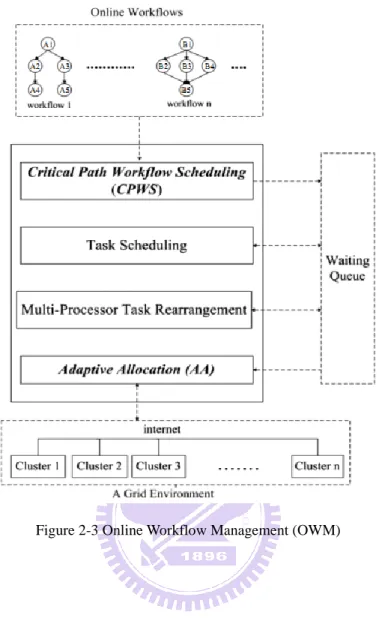
In OWM, there are four processes: Critical Path Workflow Scheduling (CPWS), Task Scheduling, Task Rearrangement and Adaptive Allocation (AA). Figure 2-3 shows the structure of OWM. CPWS manages the task interdependence and submits tasks into waiting queue according to the critical path in workflows. The task scheduling process in OWM sorts waiting queue like RANK_HYBD. In the task-parallel task scheduling, there may have some slacks among the tasks when the free processes are not enough for the first task in the waiting queue. The multi-processor task rearrangement process works for minimizing the slacks with latter tasks in the queue to improve utilization. When there are free resources, AA takes the highest priority task in the waiting queue, and selects the required resources to execute the task.

(21)

11

(22)

12

Chapter 3 Mixed-Parallel Online Workflow

Scheduling

In this chapter, we propose a Mixed-parallel Online Workflow Scheduling (MOWS) approach. According to OWM [12], we also divides the mixed-parallel online workflow scheduling problem into four phases: task prioritizing, waiting queue scheduling, task rearrangement, and task allocation, as shown in Figure 3-1. MOWS adopts SWS [9][12] in the task prioritizing phase and develops four new strategies for the other three phases: (1) shortest-workflow-first scheduling, (2) priority-based backfilling, (3) preemptive task execution, and (4) all-EFT task allocation.

(23)

13

3-1 Shortest-Workflow-First Strategy

The waiting queue scheduling phase in OWM adopts RANK_HYBD [9]. RANK_HYBD calculates the rank value of each task according to the definition in HEFT [2]. If all of the tasks in the waiting queue come from the same workflow, the scheduler sorts the tasks in non-ascending order by the rank value. On the other hand, if there are multiple workflows in the queue, the tasks are sorted in non-descending order according to their rank values. In an extreme case where all workflows are actually single jobs, the RANK_HYBD approach is equivalent to the Shortest Job

First (SJF) policy [30]. However, for general workflows with more than one job, the

SJF policy can‟t always be guaranteed in RANK_HYBD since a task with a lower rank value may come from a larger workflow and the tasks from different workflow may be interleaved with each other.

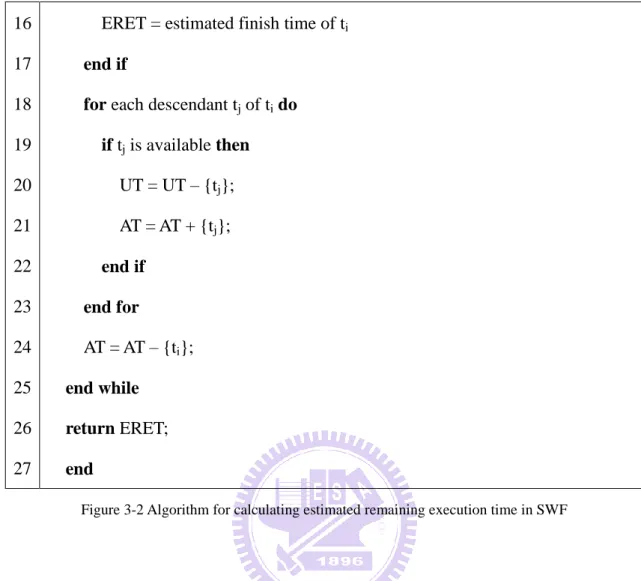
In this thesis we propose a Shortest-Workflow-First (SWF) strategy which enforces the SJF policy in the waiting queue scheduling phase in order to reduce the average makespan of all workflows. SJF is a well-known scheduling policy which is especially appropriate for batch tasks [30]. In SWF, the scheduler calculates the estimated remaining execution time of each workflow whenever a new workflow is submitted to it. After that, tasks in the waiting queue are first sorted in non-descending order by the estimated remaining execution time of the workflows they belong to. Then, tasks coming from the same workflow are sorted in non-ascending order according to their rank values. Each time a task becomes ready, it is simply put into the appropriate position among the tasks of the same workflow in the waiting queue according to its rank value. Figure 3-2 describes the algorithm for calculating the estimated remaining execution time of each workflow. First, lines 5 to10 finds the

(24)

14

ready tasks for the workflow. Lines 11 to 24 runs in a loop to select the ready task with the highest rank value, map it to the resource that produces the minimal estimated finish time of that task, and check if any descendants of the task become ready until all of the tasks have been mapped.

1 2 3 4 5 6 7 8 9 10 11 12 13 14 15 W: workflow C: profile of clusters Calc_ERET(W, C) begin AT = Ø ; UT = Ø ; ERET = 0;

for each uncompleted task ti ϵ W do

if all of the ancestors of ti are completed then

AT = AT + {ti};

else

UT = UT + {ti};

end for

while (AT≠Ø) do

select ti ϵ AT where ti has the highest rank value;

MapToBestResource(ti, C); // map ti to the resource with best

performance and update profile. update estimated information of ti;

(25)

15

Figure 3-2 Algorithm for calculating estimated remaining execution time in SWF

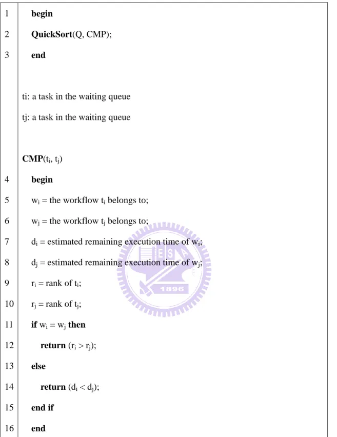
Figure 3-3 shows the task prioritizing algorithm of SWF. Line 2 sorts the waiting queue using quicksort with a customized comparison function CMP described in lines 4 to 16. The comparison function first checks if the input tasks come from the same workflow. If so, tasks are compared by their rank values and the task with higher rank value has higher priority. Otherwise, tasks are compared by the estimated remaining execution time of the workflows they belong to and the task coming from a workflow with shorter remaining time will get a higher priority.

16 17 18 19 20 21 22 23 24 25 26 27

ERET = estimated finish time of ti

end if

for each descendant tj of ti do

if tj is available then UT = UT – {tj}; AT = AT + {tj}; end if end for AT = AT – {ti}; end while return ERET; end Q: waiting queue SWF_Prioritizing(Q)

(26)

16

Figure 3-3 The task prioritizing algorithm of SWF

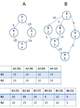
In the following, we use two example DAGs and a resource set, shown in Figure 3-4, to compare how RANK_HYBD and SWF work. The computation time of each 1 2 3 4 5 6 7 8 9 10 11 12 13 14 15 16 begin QuickSort(Q, CMP); end

ti: a task in the waiting queue tj: a task in the waiting queue

CMP(ti, tj)

begin

wi = the workflow ti belongs to;

wj = the workflow tj belongs to;

di = estimated remaining execution time of wi;

dj = estimated remaining execution time of wj;

ri = rank of ti; rj = rank of tj; if wi = wj then return (ri > rj); else return (di < dj); end if end

(27)

17

task on different clusters is given in the tables below the DAGs. The number in the parentheses next to the task name indicates the number of resources required by the task. The rank of each task calculated according to the definition in [2] is:

DAG A: A1 (75); A3 (45); A2 (40); A4 (20)

DAG B: B1 (80); B3 (60); B2 (55); B4 (25); B5 (25); B6 (5)

The scheduling results according to RANK_HYBD and SWF are shown in the two subfigures of Figure 3-5, respectively, where the width of each block represents the number of processors used and the length stands for the required execution time. In the case of RANK_HYBD, task B4 becomes ready when task B1 finishes at time 10. Then, task B4 is allocated at time 15, when task A1 finishes, since it has the smallest rank value among tasks in the waiting queue. The allocation of B4 would delay the execution of task A2 and task A3 and result in a makespan of 45 time units for DAG A as shown in the Figure 3-5. On the other hand, SWF makes sure that tasks from DAG A will have higher priority than tasks from DAG B since DAG A is smaller than DAG B. The enforcement of the SJF policy in SWF allows tasks A2 and A3 to be allocated before B4, leading to a shorter makespan for DAG A while the makespan of DAG B remains the same as shown in Figure 3-5. This would reduce the average makespan of all DAGs and improve the overall system performance.

(28)

18

Figure 3-4 Two example workflows

(29)

19

3-2 Priority-Based Backfilling

After waiting queue scheduling, the scheduler tries to allocate each task in sequence. If the number of free resources is not enough for the first task, the resources are left idle and become a schedule hole, resulting in degraded resource utilization. To resolve the problem, the task rearrangement phase is introduced to allow out-of-order execution to improve resource utilization and thus the overall system performance.

Backfilling strategies are extensively used by many SPMD based parallel job schedulers to reduce resource fragmentation by permitting tasks to run out of order as long as they do not delay certain tasks. Backfilling is traditionally used with a First-Come-First-Serve (FCFS) scheduler. Users are expected to provide estimates of task execution time. The scheduler rearranges the waiting queue according to these estimates to improve resource utilization and system performance while maintaining a certain degree of fairness. Various versions of backfilling have been proposed [31], e.g. EASY backfilling and conservative backfilling.

EASY backfilling allows a task to backfill provided that the task does not delay the first task in the waiting queue. On the other hand, conservative backfilling allows a task to backfill as long as any previous task in the waiting queue will not be delayed. In [12], OWM introduced both EASY and conservative backfilling into the task rearrangement phase. However, experiments showed that such rearrangement did not necessarily lead to performance improvement. This is because the backfilling in OWM creates an individual profile of resource usage at future times for each cluster instead of a single profile for the entire multi-cluster environment. Backfilling is traditionally used in a single cluster or parallel computer system. OWM applies the

(30)

20

concept of backfilling directly to a multi-cluster environment. Therefore, each cluster is treated individually with its own profile. The backfilling in OWM works as follows. Each task in the waiting queue is repeatedly scheduled into the profiles of all clusters to find out the best possible Earliest Start Time (EST). The tasks in the waiting queue are then allocated with the AA technique in OWM in the non-descending order of EST. However, this approach incurs some problem. Consider a scenario for OWM‟s backfilling shown in Figure 3-6, where the length of each block represents the number of processors used and the width stands for the required execution time. Notice that the width of a task may be different on different resources since the task requires different execution times on different resources in a heterogeneous environment. OWM maintains individual profiles for three resources. In this scenario, OWM will allocate task C before task B since task B would not be delayed by the backfilling according to the profile of R3, which has more processors than R1 and R2. However, since task A is given trial allocations on all three profiles, it may not actually be allocated on R3. In that case, the allocation of task C before task B might result in the delay of task B and thus deteriorate the makespan of the entire workflow. To overcome the drawback of OWM‟s backfilling, we propose a priority-based backfilling approach in the following.

(31)

21

We propose a modification to the original conservative backfilling strategy, which makes it amenable to priority-based waiting queues. The modified backfilling strategy is described below:

1. Each task in the waiting queue holds three attributes: Estimated Start Time (EST), Estimated Finish Time (EFT), and Estimated Allocated Cluster (EAC).

2. The scheduler creates a profile for the entire multi-cluster environment based on the conservative backfilling strategy, recording the estimated information of each task. The profiling algorithm is described in Figure 3-7.

3. Each time a new task is submitted into the waiting queue, the scheduler will re-create the profile and update the estimated information of tasks.

4. Then scheduler allocates tasks in the non-descending order by their estimated start time instead of their priority.

Figure 3-7 Profiling algorithm for backfilling

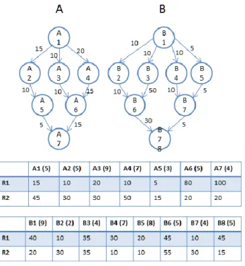
To illustrate the advantage of our backfilling approach, consider the simple DAGs shown in Figure 3-8. The computation time of each task on two different clusters and the number of resources required by each task are given in the tables

for all tasks in their order in waiting queue do

1. Find the first point where enough resources are available on some cluster. 2. Update EST, EFT, and EAC for that task.

3. Mark the resources occupied for the duration of the task's estimated execution time.

(32)

22

below the DAGs. The task ranking result of each DAG is:

DAG A: A1 (230); A4 (170); A3 (160); A6 (125); A2 (105); A5 (75); A7 (60)

DAG B: B1 (235); B3 (195); B2 (140); B6 (110); B4 (75); B5 (75); B7 (55); B8 (30)

The two subfigures in Figure 3-9 show the scheduling results of pure RANK_HYBD and RANK_HYBD accompanied with our priority-based backfilling, respectively. We also show the content of waiting queue at different time points in the two subfigures in order to illustrate the allocation sequence and backfilling activities. The blue colored tasks are allocated at that time point according to the RANK_HYBD mechanism and the red colored tasks are backfilled at the time point by our priority-based backfilling approach. The numbers of processors in R1 and R2 are 14 and 12, respectively. In the case of RANK_HYBD, task A2 is delayed since task A3 cannot be allocated at time 15, leading to a larger makespan of the overall workflow. On the contrary, with priority-based backfilling, task A2 is backfilled at time 15 since the backfilling will not delay the execution of task A3. Later, task A3 and task B3 are also backfilled at time 25. Finally, the priority-based backfilling approach achieves approximately 20% performance improvement, in terms of average makespan of the two workflows, compared to the pure RANK_HYBD approach.

(33)

23

Figure 3-8 Two example workflows

(34)

24

3-3 Preemptive Task Execution

In SWS [9], if a task with a lower rank value becomes ready and enters the waiting queue earlier than a task coming from the same workflow and having a higher rank value, the lowerly ranked task might be allocated first and hence delay the allocation of the higherly ranked task, degrading the makespan of the entire workflow. To resolve the above issue, CPWS in OWM [12] enforces that tasks of the same workflow will be put into the waiting queue in the non-ascending order of their rank values. This policy achieves performance improvement in terms of average makespan, compared to SWS, as shown in [12]. However, we found that CPWS may unnecessarily reduce the resource utilization and thus deteriorate the overall system performance since some lowerly ranked tasks are prevented from execution even though the higherly ranked tasks are not yet ready and there are enough resources for the lowerly ranked tasks. To take the advantages of both SWS and CPWS, we propose a preemptive task execution approach for the task allocation phase to cooperate with SWS used in the task prioritizing phase.

Our approach allows a lowerly ranked task to be allocated and executed before higherly ranked tasks if they are not yet ready. However, later when a higherly ranked task becomes ready, the system will suspend the lowerly ranked task to release resources for the higherly ranked task‟s immediate execution. The suspended task is put back to the waiting queue for scheduling and will be resumed later to finish its remaining computation on some available resources. This suspend-and-resume approach is achieved through the help of the virtualization technology in cloud computing environments, where virtual machines can be migrated smoothly between different machines.

(35)

25

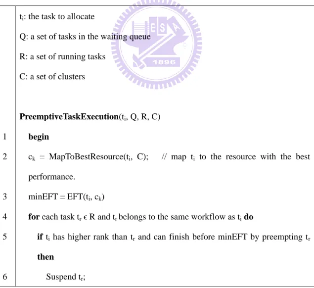
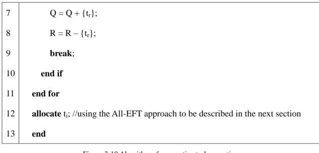
Figure 3-10 shows the algorithm of preemptive task execution. Line 2 first finds a resource which produces the minimal estimated finish time for the current task. Through lines 4 to 13, the scheduler travels the running queue to check each running task which comes from the same workflow and has a lower rank value than the current task. If the estimated finish time of the current task can be further reduced by preempting any such a running task, the scheduler then suspends that running task, first found, and moves it back to the waiting queue. Finally, the scheduler allocates the current task by the All-EFT task allocation method, which will be described in the next section. 1 2 3 4 5 6

ti: the task to allocate

Q: a set of tasks in the waiting queue R: a set of running tasks

C: a set of clusters

PreemptiveTaskExecution(ti, Q, R, C)

begin

ck = MapToBestResource(ti, C); // map ti to the resource with the best

performance.

minEFT = EFT(ti, ck)

for each task tr ϵ R and tr belongs to the same workflow as ti do

if ti has higher rank than tr and can finish before minEFT by preempting tr

then

(36)

26

Figure 3-10 Algorithm of preemptive task execution

Figure 3-11 and Figure 3-12 present an example to illustrate the differences between SWS, CPWS, and our SWS+preemptive task execution. Figure 3-11 is the information of the workflow used in the example. Figure 3-12 shows three different resultant schedules produced by the three different approaches. In this example, the order of all tasks in workflow A, from high to low rank values, is A1, A2, A4, A3, A5. In the case of SWS, A3 is allowed to be allocated before A4 although it has a smaller rank value, resulting in a makespan of 90 time units. In the case of CPWS, the allocation sequence is enforced to conform to the rank order. Therefore, A4 is allocated before A3. This arrangement leads to a shorter makespan, 70 time units, than in the case of SWS. Notice that unlike traditional parallel job allocation, the execution starting sequence may be different from the allocation sequence for workflow scheduling since tasks might have data dependency between each other. That is why in Figure 3-12 (B) it appears that A3 begin its execution before A4 although actually A4 gets its allocation before A3, because A4 has to wait for input data from A2 to start its execution. In the case of our SWS + preemptive task execution, A3 is allocated before A4 since it becomes ready earlier than A4. However, when A4 becomes ready, 7 8 9 10 11 12 13 Q = Q + {tr}; R = R – {tr}; break; end if end for

allocate ti; //using the All-EFT approach to be described in the next section

(37)

27

A3 is suspended at time 35 to release resources for A4. A3 is resumed later on another resource at time 40. Since the SWS + preemptive task execution approach guarantees the priority of A4 without sacrificing resource utilization, it achieves the best makespan, 65 time units, among the three approaches.

(38)

28

Figure 3-12 A comparison of SWS, CPWS, and preemptive task execution

3-4 All-EFT Task Allocation

In the task allocation method of OWM, which is called AA, when there are more than one cluster being able to accommodate a task, the scheduler allocates the task to the cluster among them which can lead to the earliest estimated finish time. If there is only one cluster that can accommodate the task, the scheduler will calculate the earliest estimated finish time of the task on each cluster in the system and allocate the task to the cluster with the earliest estimated finish time.

In this thesis, we adopt an All-EFT approach, which always considers each cluster in the system and allocates the task to the cluster leading to the earliest

(39)

29

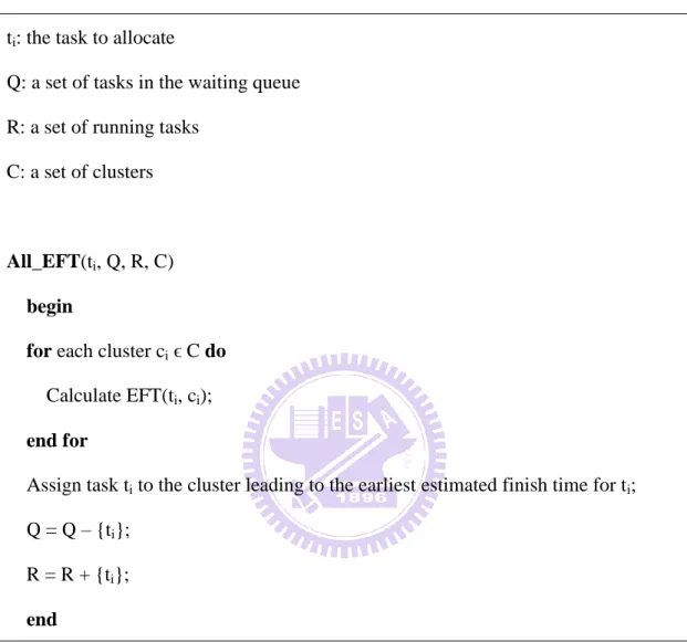
estimated finish time. Figure 3-13 describes the All-EFT approach in an algorithmic style.

Figure 3-13 All-EFT algorithm

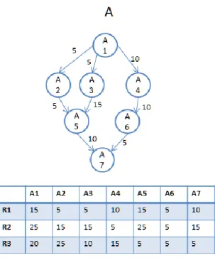
Considering a simple workflow given in Figure 3-14, the ranking list of tasks is {A1, A3, A2, A4, A5, A6, A7}. Figure 3-15 shows the scheduling results obtained from AA and All-EFT task allocation, respectively. According to the ranking list, at time zero A1 is allocated first. At time 15, three tasks, A3, A2, and A4, become ready and A3 is allocated first according to their rankings. When trying to allocate A2, in the case of AA, it is allocated to resource R2, since more than one cluster, R2 and R3, has

ti: the task to allocate

Q: a set of tasks in the waiting queue R: a set of running tasks

C: a set of clusters

All_EFT(ti, Q, R, C)

begin

for each cluster ci ϵ C do

Calculate EFT(ti, ci);

end for

Assign task ti to the cluster leading to the earliest estimated finish time for ti;

Q = Q – {ti};

R = R + {ti};

(40)

30

enough processors at time 15 and AA picks up the best one among them. Notice that although the allocation decision is made at time 15, A2 starts its execution at time 20 on R2 because of data communication cost. On the other hand, All-EFT allocates A2 to resource R1, starting execution at time 20, despite it is occupied at time 15 when making the allocation decision. Such allocation of A2 allows A2, A5, and A7 to finish their execution earlier, leading to a shorter makespan of the overall workflow. In Figure 3-15, the makespan produced by All-EFT task allocation is 15% less than that produced by AA.

(41)

31

(42)

32

Chapter 4 Software Simulator

This chapter presents the software simulator that we developed for simulating the workflow scheduling process in a multi-cluster platform. The simulator will be used to conduct various simulation experiments for evaluating the proposed workflow scheduling algorithms in the next chapter. Section 4-1 depicts major components in the simulation process. Section 4-2 describes the classes used to implement the components in the simulator, and Section 4-3 presents the simulation process.

4-1 Major Components in the Workflow Scheduling Process

Input Workload

A workflow application is represented by a DAG G = (V, E), where V is a set of nodes, each representing a task, and E is a set of edges, each defining the computation precedence order between two tasks.

Global Clock

In a discrete-event based simulation, the simulator maintains a global clock, and the operation of a system is represented as a chronological sequence of events. The simulator runs in a loop to remove the smallest time-stamped event from the event queue and process it. Each round the simulator processes the event; it sets the global clock to the time-stamp of the event.

Scheduler

The scheduler maintains the task interdependence in each workflow and calls the chosen algorithm to schedule the workflows. It is instrumented with some protection mechanisms for detecting the possible implementation errors of the scheduling and

(43)

33

allocation algorithms. If the allocation made by the chosen algorithm is unreasonable, e.g. a task starts its execution before receiving all the data from its parents, the scheduler throws an error message and stops the simulation.

Multi-cluster Environment

A multi-cluster platform consists of several clusters, in which each cluster may be composed of different amount of homogeneous processors. All of the clusters are fully connected through heterogeneous network links with different bandwidths and latencies.

4-2 Classes in the simulator

In this section, the classes used in the simulator are described, including DAG, EventQueue, Scheduler, DecisionMaker, and Cluster classes.

4-2-1. DAG

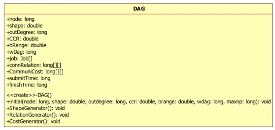
DAG provides methods to generate input workloads and stores the generated workflows including tasks and edges. Figure 4-1 shows an UML diagram of class DAG.

(44)

34 DAG +node: long +shape: double +outDegree: long +CCR: double +bRange: double +wDag: long +job: Job[] +connRelation: long[][] +CommuniCost: long[][] +submitTime: long +finishTime: long <<create>>-DAG()

+initial(node: long, shape: double, outdegree: long, ccr: double, brange: double, wdag: long, maxnp: long): void +ShapeGenerator(): void

+RelationGenerator(): void +CostGenerator(): void

Figure 4-1 Class DAG

The attributes and operations in class DAG are described as following:

Attributes

1. node: the number of tasks in the DAG.

2. shape: a number controlling the shape of the DAG. If shape > 1, it generates a shorter graph with a high parallelism degree. Otherwise, it generates a longer graph with a low parallelism degree.

3. outDegree: the maximum number of immediate descendants of a task. 4. CCR: communication cost to computation cost ratio.

5. bRange ( ): distribution range of computation costs of tasks on clusters. It is the heterogeneous factor for cluster speeds. A large range indicates significant differences in task‟s computation costs on different clusters.

6. wDAG: the average computation cost of the DAG.

7. Job: tasks and their estimated computation costs in the DAG. 8. connRelation: computation precedence order between tasks. 9. CommuniCost: estimated sizes of data transfers between tasks. 10. submitTime: the submission time of the DAG.

(45)

35 11. finishTime: the finish time of the DAG.

Operations

1. initial(): an operation that randomly generates a DAG according to the input parameters mentioned above. It receives all the parameters needed for generating a DAG and invokes ShapeGenerator(), RelationGenerator() and CostGenerator() with input parameters.

2. ShapeGenerator(): an operation that generates the shape of a DAG using the two parameters, node and shape. The height (depth) of a DAG is randomly generated from a uniform distribution with mean value equal to . The width for each level is randomly generated from a uniform distribution with mean value equal to . If Shape > 1, it generates a shorter graph with a high parallelism degree. Otherwise, it generates a longer graph with a low parallelism degree.

3. RelationGenerator(): an operation that generates the computation precedence order of a DAG according to the input parameters: node and outDegree. The number of immediate descendants of each task is randomly generated from a uniform distribution with the range [1, outDegree] .

4. CostGenerator(): an operation that generates the computation costs and the communication costs of a DAG. The average estimated computation cost of each task , i.e. , is randomly generated from a uniform distribution ranging between [1, 2 * wDag]. The estimated computation cost of each task on each cluster , i.e. , is randomly generated from a uniform distribution with the range:

(46)

36

4-2-2. EventQueue

EventQueue maintains a global system clock and processes the Event instances generated during the simulation process, of which each contains 4 attributes <type, time, dagIndex, jobIndex>. Each time an event occurs, EventQueue invokes the scheduler to simulate the scheduling process. The structures of the EventQueue class and Event class are shown in Figure 4-2.

Event +type: eventType +time: long +dagIndex: long +jobIndex: long <<create>>-Event()

<<create>>-Event(e: eventType, t: long, j: long, d: long)

EventQueue

+time: long

-queue: std::list<Event> <<create>>-EventQueue() +enQueue(e: Event): void +deQueue(): Event +remove(e: Event): void +size(): unsigned

+process(dag: DAG, dagNo: long, sched: Scheduler): void

Figure 4-2 The EventQueue class and Event class

Attributes

1. time: the global system clock.

2. queue: a priority queue storing a set of Event instances. The event with the smallest time-stamp has the highest priority.

Operations

1. enQueue(E): an operation that inserts a new event E into the queue.

2. deQueue():an operation that removes and returns the event with the smallest time-stamp.

3. remove(E): an operation that removes the event E from the queue. 4. size():an operation that returns the size of the queue.

(47)

37 the event queue and processes it.

4-2-3. Scheduler

The Scheduler maintains the task interdependence in a workflow and manages the waiting queue and running queue. When a task becomes ready, the Scheduler puts it into the waiting queue. Later, when a task begins its execution, the Scheduler moves it into the running queue. When an exit node of a workflow finishes, the Scheduler will calculate the makespan of the workflow. The Scheduler does not make a scheduling decision by itself; instead it invokes DecisionMaker to make a scheduling decision. Moreover, the scheduler is instrumented with some protection mechanisms for detecting the possible implementation errors of the scheduling and allocation algorithms. If the allocation made by DecisionMaker is unreasonable, e.g. a task starts its execution before it becomes ready, the Scheduler throws an error message and stops the simulation. Figure 4-3 shows Scheduler class.

(48)

38 Scheduler +dagNo: long +clusterNo: long +dag: DAG[] +cluster: Cluster * +eventQueue: EventQueue * +decisionMaker: DecisionMaker * +waitq: std::list<queueNode> +runq: std::list<queueNode>

<<create>>-Scheduler(cluster: Cluster, clusterNo: long, eventQueue: EventQueue, decisionMaker: DecisionMaker) +enQueue(Job): void

+remove(Job): void +size(): unsigned +front(): Job

+calc_ccCost(t: long, dagIndex: long, jobIndex: long, cluster: Cluster, clusterNo: long, realtime: bool): long +jobMapping(): void

+dagSubmit(t: long, dag: DAG): void

#jobSubmit(t: long, dagIndex: long, jobIndex: long): void +reschedule(t: long): void

#jobSelect(t: long): queueNode

+jobAllocate(t: long, dagIndex: long, jobIndex: long): bool #jobCancel(t: long, dagIndex: long, jobIndex: long): void +jobFinish(t: long, dagIndex: long, jobIndex: long): void

Figure 4-3 Class Scheduler

Attributes

1. dagNo: the total number of workflows. 2. clusterNo: the total number of clusters.

3. eventQueue: a pointer pointing to the EventQueue instance. 4. decisionMaker: a pointer pointing to the DecisionMaker instance. 5. waitq: a set of ready tasks.

6. runq: a set of running tasks.

Operations

1. enQueue(T): an operation that adds a ready task T into the waiting queue and invokes the prioritizing operation supported by DecisionMaker.

2. remove(T): an operation that removes a task T from the waiting queue and invokes the prioritizing operation supported by DecisionMaker.

3. size(): an operation that returns the size of the waiting queue. 4. front(): an operation that returns the first task in the waiting queue.

(49)

39

5. calc_ccCost(t, dagIndex, jobIndex, Cluster, i, realtime): an operation that calculates the Earliest Start Time of task <dagIndex, jobIndex> on the ith cluster Ci. If the input parameter realtime is true, the Scheduler assumes that

data transfer starts at time t. Otherwise, the Scheduler assumes that the data transfer starts right after the parents of the task finish.

6. jobMapping(): an operation that maps all of the submitted workflows to the clusters before execution. This operation is called by EventQueue before processing all of the Event instances and only for static scheduling algorithms. 7. dagSubmit(t, W): an operation that submits a workflow W to the Scheduler at time t. This operation invokes DecisionMaker::_dagSubmit() and jobSubmit() to put the entry task into the waiting queue.

8. jobSubmit(t, T): an operation that puts a ready task T into the waiting queue at time t and invokes DecisionMaker::_jobSubmit().

9. reschedule(): an operation that runs in a loop to find if there are any tasks to be allocated at current time point. Every time before the global system clock is increased, EventQueue will call this operation automatically.

10. jobSelect(): an operation that invokes DecisionMaker::_jobSelect() to select tasks from the waiting queue for allocation. This operation is continuously called by reschedule() until no more tasks can be allocated at current time point.

11. jobAllocate(t, T): an operation that invokes DecisionMaker::_jobAllocate() to allocate task T and moves task T from the waiting queue to the running queue at time t. This operation is called by reschedule() after selecting a task from the waiting queue.

12. jobFinish(t, T): an operation that removes task T from the running queue and checks if any of its immediate descendants is ready. It will invoke jobSubmit()

(50)

40 if any task becomes ready.

4-2-4. DecisionMaker

The DecisionMaker class supplies a set of interfaces to Scheduler for making a scheduling decision. Algorithms like HEFT, RANK_HYBD, and OWM can be realized by implementing some or all of the operations defined in the DecisionMaker class. The structure of the DecisionMaker class is shown in Figure 4-4.

DecisionMaker

+name: std::string +sched: Scheduler * <<create>>-DecisionMaker() +_jobMapping(): void

+_dagSubmit(t: long, dagIndex: long): void

+_jobSubmit(t: long, dagIndex: long, jobIndex: long): void +_jobSelect(t: long): queueNode

+_jobAllocate(t: long, dagIndex: long, jobIndex: long): void +_afterAllocate(node: queueNode): void

+_jobFinish(t: long, dagIndex: long, jobIndex: long): void

Figure 4-4 Class DecisionMaker

Attributes

1. name: the name of the implemented scheduling algorithm. 2. sched: a pointer pointing to the Scheduler instance.

Operations

1. _jobMapping(): an operation that maps all of the submitted workflows to the clusters before execution. This operation is only used for the static scheduling algorithms.

2. _dagSubmit(W): an operation that is called when a new workflow W is submitted to the Scheduler. Our SWF approach implements this operation to

(51)

41

calculate the estimated remaining time of uncompleted workflows.

3. _jobSubmit(T): an operation that is called when a new task T becomes ready. CPWS is realized in this operation.

4. _jobSelect(): an operation that selects a task from the waiting queue for allocation. Priority-based backfilling is achieved in this operation.

5. _jobAllocate(T): an operation that selects a cluster to accommodate task T. This operation usually invokes Scheduler::calc_ccCost() repeatedly to find the best cluster for task T.

6. _afterAllocate(T): an operation that is called after a task T has been allocated. CPWS implements this operation to remove tasks from the self-maintaining waiting queue.

7. _jobFinish(T): an operation that is called when a task T has completed its execution.

4-2-5. Cluster

The Cluster class records the resources usage and calculates the Earliest Start Time (EST) of a task according to current resource allocation profile. Figure 4-5 shows the Cluster class.

(52)

42 Cluster +np: long +CommuniRate: long[] -profile: std::list<profileNP> -jobs: std::list<profileJob> <<create>>-Cluster() +initial(): void

+submitJob(dagIndex: long, jobIndex: long, start: long, end: long, np: long): bool +cancelJob(dagIndex: long, jobIndex: long): bool

+est(start: long, duration: long, np: long): long +availableNP(t: long): long

-profileInsert(start: long, end: long, np: long): bool -profileRemove(start: long, end: long, np: long): bool

Figure 4-5 Class Cluster

Attributes

1. np: the total number of resources of the cluster.

2. CommuniRate: bandwidths of different network links connected to other clusters. 3. profile: a resource allocation profile.

4. jobs: a set of tasks running on this cluster.

Operations

1. submitJob(T, tstart, tend): an operation that tries to allocate a task T to the cluster.

The execution of task T starts at time tstart, and finishes at time tend. This

operation returns false if the number of available resources is not enough for task T during the time period between tstart and tend.

2. cancelJob(T, t): an operation that cancels a task T and releases the resources used by task T at time t.

3. est(t, duration, np): an operation that calculates the Earliest Start Time (EST) of a task since time t.

4. availbleNP(t): an operation that returns the number of available resources at time t.

(53)

43 profile.

6. profileRemove(): an operation that removes a resources allocation record from the profile.

4-3 Simulation Process

This section describes the simulation process. The simulation process involves several aforementioned classes. The EventQueue class maintains the global system clock and processes events by invoking the Scheduler class and DecisionMaker class. The following describes the details.

4-3-1. Simulation skeleton

First, the simulator constructs a multi-cluster environment and generates a sequence of input workflows using the DAG class. Then, it initiates the corresponding Scheduler instance and DecisionMaker instance for the scheduling algorithm to be simulated. Finally, it initiates an EventQueue instance to handle the events generated during the simulation. Figure 4-6 shows the pseudo code of the discrete-event handling process (EventQueue::process()). In the process, EventQueue first checks the submission time of each workflow in line 2 to line 10. If the submission time of a workflow is 0, the workflow is submitted to the Scheduler right away. Otherwise, EventQueue creates an event indicating the submission of the workflow at the specified time point. Line 11 invokes the Scheduler::jobMapping() operation to support static algorithms before any event handling process. Then EventQueue sets the global system clock to 0 in line 12 and starts to handle events in line 13.

Each time the EventQueue handles an event, it checks if the time stamp of the event is larger than the global system clock. If it is, the EventQueue will invoke the

(54)

44

Scheduler::reschedule() operation to check if there are any ready tasks to be allocated at current time point. Scheduler::reschedule() runs in a loop to select a task for allocation each time until the resources are not enough. Then the EventQueue sets the global system clock to the time stamp of the event in line 20. Line 22 to 26 shows that if the event is a „submit‟ event, EventQueue invokes the Scheduler::dagSubmit() operation to submit the workflow to the Scheduler; if the event is an „end‟ event, EventQueue invokes the Scheduler::jobFinish() operation to check if there are tasks becoming ready for submission. The pseudo code only shows the generation of workflow submission events explicitly in line 7. The task submission and ending events are generated inside the operations of SCHED. The discrete-event handling process continues until all of the events have been handled.

(55)

45 1 2 3 4 5 6 7 8 9 10 11 12 13 14 15 16 17 18 19 20 21 W: input workflows SCHED: the scheduler

EventQueue::Process(W, SCHED) begin

for each workflow wi ϵ W do

t0 = submission time of wi;

if t0 = 0 then

submit wi to SCHED

else

insert an event, which submits wi to SCHED at time t0, into this->queue;

end if end for

SCHED->jobMapping(); this->time = 0;

while event queue ≠ Ø do

ej = this->deQueue(); wj = workflow of ej; jj = task of ej; tj = time of ej; if tj > this->time then SCHED->reschedule(); this->time = tj; end if

(56)

46 22 23 24 25 26 27 28 SCHED->dagSubmit(tj, wj);

else if type of ej = END then

SCHED->jobFinish(tj, wj, jj);

end if end while end

Figure 4-6 Pseudo code of EventQueue::process()

4-3-2. Workflow Processing

In the simulator, the task interdependence in the workflows is maintained by the Scheduler class. When a new workflow is submitted by calling Scheduler::dagSubmit(), the scheduler finds the entry task of the workflow and puts it into the waiting queue by Scheduler::jobSubmit(). Scheduler::jobSelect() and Scheduler::jobAllocate() are used in the Schduler::reschedule() to allocate ready tasks to the clusters and move the allocated tasks from the waiting queue to the running queue in the event handling process. When a task finishes its execution, Scheduler::jobFinish() is invoked to check if any descendants become ready and invoke Scheduler::jobSubmit() to put the ready descendants into the waiting queue. Figure 4-7 shows the flow chart of the workflow processing procedure in the simulator.

(57)

47

(58)

48

Chapter 5 Performance Evaluation and

Discussion

This chapter evaluates the proposed methods in our MOWS and compares them with the approaches used in OWM [12]. Section 5-1 introduces the setup for the following experiments and the metrics used in the performance analysis. Section 5-2 presents the experimental results of the proposed methods in MOWS.

5-1 Experimental Setup and Performance Metrics

5-1-1. Algorithms under Evaluation

In addition to the overall effects of MOWS, we also evaluated the effectiveness of each proposed method in it separately in the following experiments. Therefore, we implemented various online workflow scheduling approaches which differ with each other in the methods used in the four scheduling phases. The following describes the implemented approaches and the corresponding methods used in the four scheduling phases. :

 OWM: adopting CPWS, RANK_HYBD, FCFS, and AA in the four

scheduling phases, respectively.

 OWM(SWF): replacing RANK_HYBD with SWF in the phase of waiting

queue scheduling, used to evaluate the effectiveness of the SWF strategy through comparing it with OWM.

 OWM(backfilling): replacing FCFS with priority-based backfilling in the

phase of task rearrangement, used to evaluate the effectiveness of the priority-based backfilling strategy through comparing it with OWM.