The Fading Number of Memoryless
Multiple-Access General Fading Channels
非記Ȧሗ多重存取廣義衰減通道之衰減數
The Fading Number of Memoryless
Multiple-Access General Fading Channels
研
究 生:黃昱銘
Student : Yu-Ming Huang
指導教授:Ǒ詩台方
教授
Advisor : Prof. Stefan M. Moser
ῗ 立 交 通 大 學
電 信 工 程 學 系 碩 士 ჟ
碩 士 ࣧ ᅎ
⑸
ḋ
Submitted to Institution of Communication Engineering
College of Electrical Engineering and Computer Science
National Chiao Tung University
In partial Fulfillment of the Requirements
for the Degree of
Mater of Science
in
Communication Engineering
June 2013
Hsinchu, Taiwan, Republic of China
中ဝ
ῗ一࿇二年六月
Information Theory
Laboratory
Institute of Communication Engineering National Chiao Tung University
Master Thesis
The Fading Number of
Memoryless Multiple-Access
General Fading Channels
Huang Yu-Ming
Advisor: Prof. Dr. Stefan M. Moser
National Chiao Tung University, Taiwan Graduation Prof. Dr. Hsie-Chia Chang
Committee: National Chiao Tung University, Taiwan Prof. Dr. Chia-Chi Huang
中
中
中文
文
文摘
摘
摘要
要
要
非
非
非記
記
記憶
憶
憶型
型
型多
多重
多
重
重存
存
存取
取
取廣
廣
廣義
義
義衰
衰
衰減
減
減通
通
通道
道
道之
之
之衰
衰
衰減
減
減數
數
數
研究生:黃昱銘
指
導教授:莫詩台方 博士
國立交通大學電信工程研究所碩士班
本篇論文中探討的是非同調多重存取廣義規律衰減通道的通道容量。其中傳送端的使 用者允許擁有任意數量的天線,但接收端僅允許擁有一條天線。在此通道中,所傳送的訊 號會遭遇相加高斯雜訊以及非記憶型廣義衰減的影響,也就是說,此衰減不被特定的機率 分布所限制,如雷利(Rayleigh)分布及萊斯(Rician)分布。雖然我們假設對於時間來說 為非記憶性,但我們允許對於空間上的記憶,也就是說,對於不同天線的衰減分布是相關 的。在傳送端使用者之間不允許相互合作通訊,因此各使用者假設在統計特性上獨立。 我們的研究是根據已知的單使用者廣義衰減通道的漸進通道容量,推廣到多使用者多重 存取的總通道容量,且允許傳送端使用者擁有多餘一條的天線數。我們知道在此通道下, 增加可使用功率對於通道容量的成長是極沒效率的,僅以雙對數形式增長,此外,在高訊 雜比時,漸進總通道容量中的第二項數值,我們稱之為衰減數。我們成功證明在此通道下 的衰減數與單使用者的衰減數相同。 此研究結論在考量三種功率限制下皆成立,分別為尖峰值功率限制,時間平均功率限 制,以及允許功率分享的時間平均功率限制。其中第三項限制是不實際的因為它代表我們 允許使用者分享功率卻不允許合作,但它有助於我們的推導且我們可證明結果皆一致。 我們的證明是基於互消息的對偶型上界與輸入信號的機率分布逃脫到無限的觀念,其精 神為當可用的功率趨近於無限大時,輸入信號必定會使用趨近於無限大的符號。Abstract
The Fading Number of Multiple-Access
General Fading Channels
Student: Huang Yu-Ming
Advisor: Prof. Stefan M. Moser
Institute of Communication Engineering
National Chiao Tung University
In this thesis, the sum-rate capacity of a noncoherent, regular multiple-access general fading channel is investigated, where each user has an arbitrary number of antennas and the receiver has only one antenna. The transmitted signal is subject to additive Gaussian noise and fading. The fading process is assumed to be general and memoryless, i.e., it is not restricted to a specific distribution like Rayleigh or Rician fading. While it is memoryless (i.e., independent and identically distributed IID) over time, spacial memory is allowed, i.e., the fading affecting different antennas may be dependent. On the transmitter side cooperation between users is not allowed, i.e., the users are assumed to be statistically independent.
Based on known results about the capacity of a single-user fading channel, we derive the exact expression for the asymptotic multiple-user sum-rate capacity. It is shown that the capacity grows only double-logarithmically in the available power. Futhermore, the second term of the high-SNR asymptotic expansion of the sum-rate capacity, the so-called fading number, is derived exactly and shown to be identical to the fading number of the single-user channel when all users apart from one is switched off at all times.
The result holds for three different power constraints. In a first scenario, each user must satisfy its own strict peak-power constraint; in a second case, each user’s power is limited by an average-power constarint; and in a third situation — somewhat unrealistically — it is assumed that the users have a common power supply and can share power (even though they still cannot cooperate on a signal basis).
The proof is based on a duality-based upper bound on mutual information and on the concept of input distributions that escape to infinity, meaning that when the available power tends to infinity, the input must use symbols that also tend to infinity.
Acknowledgments
My advisor, Prof. Stefan M. Moser, is the best. He always has unbelievable intuition in information theory, and always answers my quesions patiently, and the most important thing is that he always gives me confidence in researches, and always trusts that I am able to solve problems by myself. Furthermore, he teaches me not only specialize knowledge but the attitude about facing challenge, he lets me know how to enjoy research, and he treats me just like a real family.
I also thank all the members in the Information Theory LAB. They have helped me a lot when I was stuck in research problems, and I really enjoy those times with all of you, no matter what we were doing. Moreover, I really appreciate my girl friend Yun-Shan. She has always encouraged me when I am depressed, and never complain whenever I sat working on my computer, with mythoughts far away.
Finally, I would like to thank my parents, my grandparents and my brothers. Without their support, I could not have finished my master degree. I am greatly indebted to my families.
Hsinchu, 28th June 2013
Contents
Acknowledgments III
1 Introduction 1
1.1 Introduction & Background . . . 1
1.2 Notation . . . 3
2 Channel Model 5 2.1 The General Channel Model . . . 5
2.2 A Simple Special Case of the Channel Model . . . 6
2.3 Discussion on Power Constraints . . . 6
3 Mathematical Preliminaries & Previous Results 9 3.1 The Channel Capacity . . . 9
3.2 The Fading Number . . . 11
3.3 Escaping to Infinity . . . 12
3.4 Generalization of Escaping to Infinity to Multiple Users . . . 14
3.5 An Upper Bound on the Sum-Rate Capacity and Fading Number . . . 14
3.6 The Fading Number of Rician Fading SISO MAC . . . 15
4 Main Result 16 4.1 Natural Upper and Lower Bounds . . . 16
4.2 An Upper Bound on the Fading Number for Our Channels . . . 17
4.3 The Fading Number of General Fading MAC . . . 17
5 Derivation of Results 19 5.1 Derivation of Theorem 4.1 . . . 19
5.2 Derivation of Theorem 4.2 and Corollary 4.3 . . . 22
6 Discussion and Conclusion 31
A Derivation of Equation (5.58) 34
Introduction Chapter 1
Chapter 1
Introduction
1.1
Introduction & Background
Wireless communication channels encounter additive Gaussian noise and a phenomenon called fading. The fading phenomenon impacts the signal amplitude (often destructively) and is usually modeled as multiplicative noise. Due to this multiplicative noise, it is much more difficult to design a good communication system for such channels, and hence fading is a hot research topic. Usually channels with this fading phenomenon are called fading channels.
In this thesis we investigate a multiple-access fading channel. We do not restrict our models to any kind of fading processes. This means that the multiplicative noise process can have any arbitrary random distribution, and the fading processes are allowed to be dependent on each other.
Multiple-access indicates that several users utilize the channel at the same time. These users are assumed to be statistically independent, which distinguishes the multiple-user channel from the channel with a single user having multiple antennas. Common examples of the multiple-access channel (MAC) are a group of mobile phones communicating with a base station or a satellite receiver with several ground stations.
The work in this thesis focuses on the capacity analysis of the multiple-access fading channel. The concept of channel capacity was initially introduced in Shannon’s famous landmark paper “A Mathematical Theory of Communication” [1]. In this paper, Shannon proved that for every communication channel there exists a theoretical maximum rate — denoted capacity—that can be transmitted reliably, i.e., for every transmission rate below capacity, the probability of making a decision error can be as small as one wishes. Therefore, the capacity is fundamental for the understanding of the channel and also for the judgment of efficiency for a designed system on a channel. However, capacity is defined in a single-user system. To generalize it to a multiple-user situation, we consider the theoretically maximum possible sum rate of all users. To be specific, we call this maximum possible sum rate the sum-rate capacity, but simply use capacity exchangeably in both cases.
communica-1.1 Introduction & Background Chapter 1
tion channel, the channel capacity of a general fading channel is not yet known. Researchers have been trying to solve this problem via various approaches. One common approach is to analyze the channel based on the assumption that the receiver has perfect knowledge of the channel state by estimating the channel state from training sequences. However, we cannot ignore the bandwidth kept for these training sequences. Furthermore, we can never measure the channel state perfectly even with a large amount of training data.
Another approach is to utilize joint estimation and detection: here we estimate the chan-nel state by the received information data. No assumption of a particular estimation scheme is then required. The only assumption is that both the transmitter and the receiver know the channel characteristics (but not the realizations!). The capacity under this approach of analysis is known as the noncoherent capacity.
So far, no exact expression for the noncoherent capacity of a fading channel is known. As a function of the signal-to-noise ratio (SNR), the noncoherent capacity is only understood at asymptotic high and low SNR. Lapidoth and Moser have derived in [2] [3] [4] the asymptotic high-SNR capacity of general single-user fading channels. The asymptotic low-SNR capacity of fading channel has also been derived in [5]. In this work we extend the result of the high-SNR asymptotic capacity to the multiple-access channel. It is the generalization of the result about the Rician fading MAC, which is given in [6].
The evaluation of noncoherent capacity involves an optimization problem. To derive the exact expression either analytically or numerically is very difficult. One promising approach is to derive upper and lower bounds to the capacity and try to make them close. Based on [7], we know natural lower and upper bounds from the single-user multiple-input single-out (MISO) channel and the multiple-user MISO channel. There the lower bound is the capacity when only the user with best channel transmits, and the other users swithch off, and the upper bound is the capacity under the assumption of all users are allowed to cooperate, i.e., we view the multiple-access channel as a MISO channel. We also know that the upper bound from the MISO channel is loose. The technique of deriving upper bounds of mutual information is based on duality, a successful technique [8], [3] utilizing the dual expression of the channel capacity where the maximization (of mutual information) over distributions on the channel input alphabet is replaced with a minimization (of average relative entropy) over distributions on the channel output alphabet. In [6] and [9], the fading number in multiple-access Rician fading channel are derived, but the fading process is restricted to Gaussian fading, which is far from a realistic assumption in an environment for countryside or in places near the receiver, where not many obstacles between transmitter and receiver. Hence, we have to loosen the assumption about the fading process, and that is the reason why we insist on the general fading case.
The fading number is defined as the second term in the high-SNR asymptotic capacity and is independent of SNR. It can be an indicator to get more insight about what is the most efficient way to transmit in such fading channel models. As the main contribution in this thesis, we obtain the fading number and asymptotic capacity of multiple-access general fading channel, where users are allowed to have more than one antenna (each user can be viewed as a MISO case individually, not SISO).
1.2 Notation Chapter 1
The structure of this thesis is as follows. In the remainder of this chapter, we will briefly describe our notation. Next we will give the setup of the channel model in Chapter 2. Furthermore, there is a discussion on power constraints in the end of this chapter. The subsequent Chapter 3 gives some mathematical preliminaries about the sum-rate capacity, the fading number and input distributions that escape to infinity. Moreover, we review the previous results as the fundamental basis of this thesis and state some important preliminary results as well. The main result and its derivation are shown in Chapter 4 and Chapter 5, respectively. Finally we give a discussion and conclusion in Chapter 6.
1.2
Notation
For random quantities we use uppercase letters such as X to denote scalar random variables and for their realizations we use lowercase letters like x. For random vectors we use bold-face capitals, e.g., X and bold lower-case letters for their realization, e.g., x. Constant matrices are denoted by upper-case letters but of a special font, e.g., H. For random matrices we yet use another font, e.g., H. Scalars are typically denoted using Greek letters or lower-case Roman letters.
Some exceptions that are widely used and therefore kept in their customary shape are:
• h(·) denotes the differential entropy.
• I(·; ·) denotes the mutual information functional.
Moreover, we use the capitals Q and W as the input probability distribution and the channel law (distribution of the channel output conditioned on the channel input), and C exchange-ably for the single-user capacity and the multiple-user sum-rate capacity. The energy per symbol is denoted by E, and the signal-to-noise ratio SNR is denoted by snr. Also note that we use log(·) to denote the natural logarithmic function.
Finally, the input vector of the i-th user is Xi with ni components, corresponding to
Hi of user i antenna. Sometimes we use a compact notation of an nT-vector X consisting
of all user’s vectors xi stacked on top of each other, i.e., we get a total vector X which is
expressed by X= X1 X2 .. . Xm , (1.1)
where Xi is ni-vector, i = 1, 2, . . . m, and nT= n1+ · · · + nm.
We also use ˆXi to denote the normalized version of vector Xi to length 1, i.e.,
ˆ X1 !
X1
!X1!
1.2 Notation Chapter 1
As a warning, we would like to point out that
ˆ X"= ˆ X1 ˆ X2 .. . ˆ Xm . (1.3)
Channel Model Chapter 2
Chapter 2
Channel Model
In this chapter, we will introduce the channel model of the multiple-access general fading channel. In Section 2.1, we give the mathematical formula and some assumptions of this access channel. In Section 2.2, we will describe the special cases of the multiple-access channel when the users both in the transmitter and the receiver side use one antenna only. In Section 2.3, we discuss the power constraints.
2.1
The General Channel Model
In our analysis, we consider the noncoherent channel in the sense that both the transmitter and the receiver do not know the channel state realization, but only have knowledge about the channel characteristics, e.g., the distribution of the channel state.
We restrict ourselves to the memoryless case in our work. Distributions of the input and the channel are independent and identically distributed (IID) at every time step. Therefore, we will drop the time index.
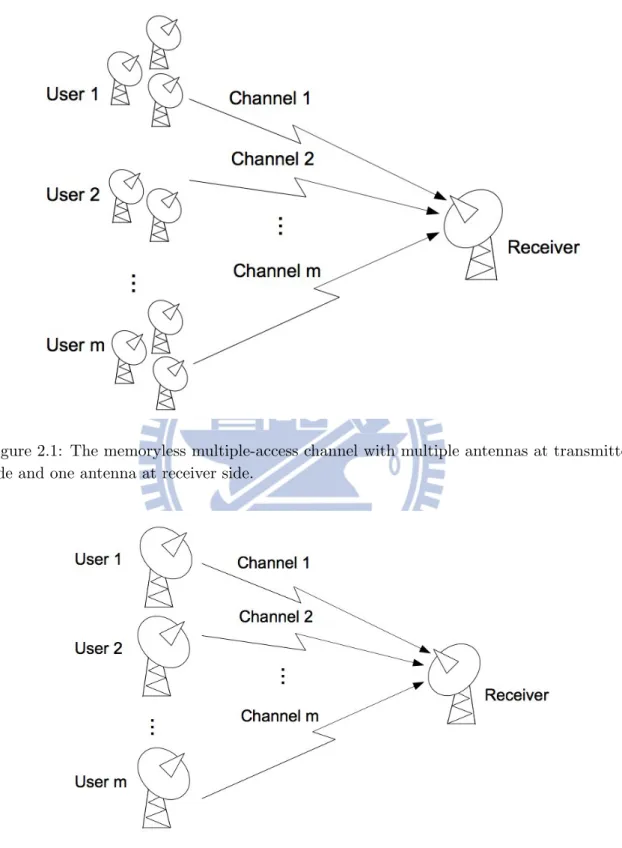
We consider a channel as illustrated in Figure 2.1 with m users, each having ni transmit
antennas for i = 1, . . . , m. The total number of transmit antennas is then
m
'
i=1
ni= nT. (2.1)
We then assume the receiver with one antenna whose output Y ∈ C is given by
Y = HTx+ Z. (2.2)
Here x ∈ CnT denotes the input vector consisting of m subvectors of length n
i for each
user; the random vector H ∈ C1×nT denotes the fading vector; the random variable Z ∈ C
denotes the additive noise.
We assume that the component of the fading H are dependent, but the additive noise Z and the fading H are independent, and that both of them are of a joint law that does not depend on the channel input x. The different users are assumed to have access to a
2.2 A Simple Special Case of the Channel Model Chapter 2
common clock, resulting in the output at a discrete time. Note that different users are not allowed to cooperate, i.e., for the input vector
X= X1 .. . Xm , (2.3)
the subvectors Xi∈ Cni denoting the input vectors of each user are statistically independent
Xi ⊥⊥ Xj, ∀ i "= j. (2.4)
We assume that the random variable Z is a spatially white, zero-mean, circularly symmetric Gaussian noise, i.e., Z ∼ NC.0, σ2/ for some σ2 >0.
As for the fading vector H, the distribution is general, with the assumption of finite power
E0!H!21 < ∞, (2.5)
and finite differential entropy
h(H) > −∞, (2.6)
the last assumption is usually denoted as regular fading.
2.2
A Simple Special Case of the Channel Model
For simplicity, we sometimes assume that each user and the receiver use only one antenna, i.e., n1 = n2 = · · · = nm = 1, such that nT= m. This reduces (2.2) to the multiple-access
SISO case. Note that
Y = HTx+ Z, (2.7)
where x ∈ Cm denotes the input vector, with n
T components xi in x are independent of
each other, but the components of H can be dependent, see Figure (2.2).
2.3
Discussion on Power Constraints
In the given setup we can consider several possible constraints on the power. We use E to denote the maximum allowed total instantaneous power in the peak-power constraint, and to denote the allowed total average power in the average-power constraint. For both cases we get
snr! E
σ2. (2.8)
Note that the total power still must be split and distributed among all users. In our channel model, we consider three different scenarios:
2.3 Discussion on Power Constraints Chapter 2
Figure 2.1: The memoryless multiple-access channel with multiple antennas at transmitter side and one antenna at receiver side.
Figure 2.2: The memoryless multiple-access channel with only one antenna at transmitter and receiver sides.
2.3 Discussion on Power Constraints Chapter 2
• Peak-Power Constraint: At every time-step, every user i is allowed to use a power of at most κi mE: Pr2!Xi!2 > κi mE 3 = 0, (2.9)
for some fixed numbers κi>0.
• Average-Power Constraint: Averaged over the length of a codeword, every user i is allowed to use a power of at most κi
mE:
E0!Xi!21 ≤
κi
mE, (2.10)
for some fixed numbers κi>0.
• Power-Sharing Average-Power Constraint: Averaged over the length of a code-word all users together are allowed to use a power of at most ¯κE:
E 4 m ' i=1 !Xi!2 5 ≤ ¯κE, (2.11)
for some fixed numbers ¯κ >0.
Note that if κi = 1 for all i, we have the special case where all users have an equal power
available. Also note that in (2.9) and (2.10) we have normalized the power to the number of user m. This might be strange from an engineering point of view; however, in regard of our freedom to choose κi, it is irrelevant, and it simplifies our analysis because we can
esaily connect the power-sharing average-power constraint with the average of the constants {κi}mi=1, i.e., if we define
¯ κ! 1 m m ' i=1 κi, (2.12)
then the three constraints are in order of strictness: the peak-power constraint is the most stringent of the three constraints in the sense of that if (2.9) is satisfied for all i = 1, . . . , m, then the other two constraints are also satisfied; and the average-power constraint is the second most strigent in the sense that if (2.10) is satisfied for all i, then also the power-sharing average-power constraint (2.11) is satisfied. In the remainder of this thesis we will always assume that (2.12) holds.
For some comments about even more general types of power constraints, we refer to the discussion in Chapter 6.
It is worth mentioning that the slackest constraint, i.e., the power-sharing average-power constraint, implicitly allows a form of cooperation: while the users are still assumed to be statistically independent, we do allow cooperation concerning power distribution. This is not very realistic (it implies that our cellphones can share batteries), however, it helps the derivation and it will turn out that the asymptotic sum-rate capacity is unchanged irrespective of which constraint is assumed. Based on this, we can choose one of the power constraint arbitrarily in our derivation, but not all of them in the same time.
Mathematical Preliminaries & Previous Results Chapter 3
Chapter 3
Mathematical Preliminaries &
Previous Results
In this chapter we review some important concepts and some related previous results, includ-ing some known result of the Rician fadinclud-ing MAC, for which case, the exact fadinclud-ing number is already provided.
The channel model considered is (2.2). In Section 3.1 we review the channel capacity and make a further generalization to the maximum possible sum rate of multiple users. In Section 3.2 we introduce the fading number. In Section 3.3 we provide the concept of input distributions that escape to infinity and a lemma which shows that under some conditions the input distribution must escape to infinity. In Section 3.4 we extend the notion of escaping to infinity to multiple users. In Section 3.5 we review a known bound of the sum-rate capacity for our case. Finally, in Section 3.6 we get the exact value of the m-user SISO MAC Rician fading number. The concepts we use in this chapter are mainly based on [2], [3], [6], and [9].
3.1
The Channel Capacity
In this section we first review the definition of channel capacity provided by Shannon in [1]. Further we give the definition of the maximum possible sum rate of the multiple-access channel; it is basically identical to the channel capacity, but takes multiple users into consideration.
Recall that in a discrete memoryless channel (DMC), the channel capacity is defined as
C! max
QX
I(X; Y ), (3.1)
where the maximization is taken over all possible input distributions QX(·). When the
concept is generalized to the continuous case, i.e., the input and output take values in continuous alphabet, a power constraint must be taken into consideration: for the peak
3.1 The Channel Capacity Chapter 3 power constraint (2.9) C! max QX Pr[|X|2 ≤E]=1 I(X; Y ), (3.2)
or for the average power constraint (2.10)
C! max
QX
E[X2
]≤E
I(X; Y ), (3.3)
where the maximization is taken over all the input distributions satisfying the constraint. In the generalization to the memoryless multiple-user channel, we use C to denote the maximum possible sum rate. The (sum-rate) capacity of the channel (2.2) is given by
C= sup
QX
I(X; Y ), (3.4)
where the supremum is taken over the set of all probability distributions on X for which the m subvectors are independent and which satisfy the power constraint, i.e.,
Pr2!Xi!2 >
κi
mE 3
= 0, (3.5)
for a peak-power constraint, or
E0!Xi!21 ≤
κi
mE, (3.6)
for an average-power constraint.
The most general concept of capacity in a multiple-access scenario is the capacity region. The capacity region of the multiple-access channel is defined to be the closure of the set of all achievable rate tuples. An example of a 2-user capacity region is provided in figure 3.3, it is a common region for 2-user MAC. Speaking precisely, we have given three fixed numbers:
I1 ! I.X(1); Y66X(2)/, (3.7) I2 ! I.X(2); Y66X(1)/, (3.8) I3 ! I.X(1), X(2); Y/. (3.9) These three numbers together with the constraints R(1)≥ 0 and R(2)≥ 0 specify a pentagon of achievable rate pairs:
R(1) ≥ 0 R(2) ≥ 0 R(1) ≤ I1 R(2) ≤ I2 R(1)+ R(2) ≤ I3 (3.10)
3.2 The Fading Number Chapter 3
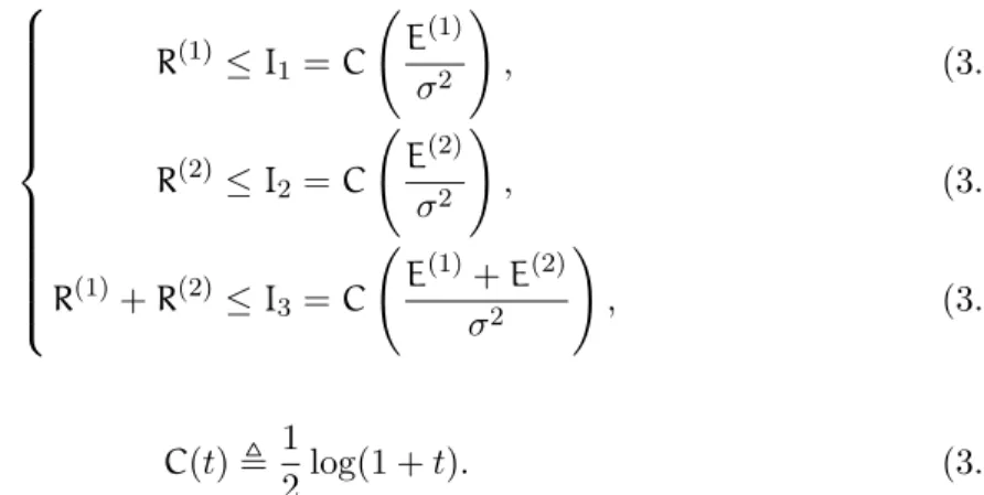
If we consider Gaussian MAC, its capacity region is given by
R(1) ≤ I1 = C ; E(1) σ2 < , (3.11) R(2) ≤ I2 = C ; E(2) σ2 < , (3.12) R(1)+ R(2) ≤ I3 = C ; E(1)+ E(2) σ2 < , (3.13) where C(t)! 1 2log(1 + t). (3.14) In the case of m users with m > 2, the capacity region is a m-dimensional pentagon, i.e., the m-user capacity region is given by the convex closure of all rate m-tuples.
R(1) R(2) I.X(1); Y6 6X(2) / I.X(1); Y/ I.X(2); Y6 6X(1) / I.X(2); Y/
Figure 3.3: An example of capacity region for 2-user MAC.
3.2
The Fading Number
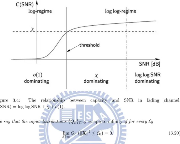
In the asymptotic analysis of channel capacity at high SNR, it has been shown in [2], [3] that at high SNR capacity grows only double-logarithmically in the SNR. This means that at high power these channels become extremely power-inefficient because we have to square the SNR to get an additional bit improvement in capacity. Furthermore, the difference between channel capacity and log log SNR is bounded as the SNR tends to infinity, i.e.,
lim
E↑∞
@
C(E) − log log E σ2
A
<∞. (3.15)
This bounded term is called the fading number. A precise definition of the fading number is as follows.
3.3 Escaping to Infinity Chapter 3
Definition 3.1. The fading number χ of a memoryless fading channel with fading matrix His defined as
χ(H)! lim
E↑∞
@
C(E) − log log E σ2
A
. (3.16)
Whenever the limit in (3.16) exists and χ is finite, the expression of capacity is
C(E) = log log E
σ2 + χ + o(1), (3.17) where o(1) denote terms that tend to zero as the SNR tends to infinity. Thus, at high SNR the channel capacity of a fading channel can be approximated by
C(E) ≈ log log E
σ2 + χ. (3.18)
Hence we can say that the fading number is the second term in the asymptotic expression of the channel capacity at high SNR. Note that the approximation of capacity in (3.18) is not always valid. In the low-SNR to medium-SNR regime, the capacity is dominated by the o(1) term that cannot be neglected in that regime. In the analysis of the asymptotic capacity, however, we are only concerned with the high-SNR regime and in particular when the SNR tends to infinity. Thus, we usually use the approximation of (3.18) instead of the intractable exact expression. Furthermore, we can even only consider the fading number because the first term of the capacity is always the same.
The fading number also plays a role as a qualitative criterion for the communication system. Since in the high-SNR regime the capacity is extremely power-inefficient, we should avoid transmission in this severe regime. The fading number can provide a threshold of how high the rate can be before entering the high-SNR regime, i.e., the fading number can provide a certain threshold snr0 such that once the available SNR is above snr0, we are in
the log log snr dominated regime, and should not stick on this system. Instead we should use other schemes, e.g., use more antennas in order to reach a higher transmission rate.
3.3
Escaping to Infinity
A sequence of input distributions parameterized by the allowed cost (in our case the cost of fading channels is the available power or the SNR, respectively) is said to escape to infinity if it assigns to every fixed compact set a probability that tends to zero as the allowed cost tends to infinity. In other words this means that in the limit—when the allowed cost tends to infinity—such a distribution does not use finite-cost symbols.
We give the definition of escaping to infinity for the fading channel under consideration in this thesis; the definition for general channels can be found in [2], [3].
Definition 3.2. Let {QE}E≥0 be a family of input distributions for the memoryless fading
channel (2.2), where this family is parameterized by the available average power E such that
EQE0!X!
3.3 Escaping to Infinity Chapter 3
Figure 3.4: The relationship between capacity and SNR in fading channel: C(SNR) = log log SNR + χ + o(1).
We say that the input distributions {QE}E≥0 escape to infinity if for every E0
lim
E↑∞QE.!X! 2≤ E
0/ = 0. (3.20)
This notion is of importance because the asymptotic capacity of fading channels can only be achieved by input distributions that escape to infinity. As a matter of fact one can show that to achieve a mutual information of only identical asymptotic growth rate as the capacity, the input distribution must escape to infinity. The following lemma describes this fact.
Lemma 3.3. Assume a single-user memoryless multiple-input multiple-output (MIMO) fad-ing channel as given in (2.2) and let W (·|·) denote the correspondfad-ing conditional channel law. Let {QE}E≥0 be a family of input distributions satisfying the power constraint (3.19)
and the condition
lim
E↑∞
I(QE, W)
log log E = 1. (3.21)
Then {QE}E≥0 escapes to infinity.
Proof. A proof can be found in [2], [3].
From the engineering point of view, this concept matches the intuition: as the available power tends to infinity, the input should utilize the resource (available power) completely, therefore any fixed symbol is not used in the limit.
3.4 Generalization of Escaping to Infinity to Multiple Users Chapter 3
Remark 3.4. When computing the bounds of the fading number (which is part of the capac-ity in the limit when E tends to infincapac-ity), we can therefore assume that for any fixed value E0
Pr.!X!2≤ E
0/ = 0. (3.22)
3.4
Generalization of Escaping to Infinity to Multiple Users
The content in this section is mainly based on [6] and [10]. The following proposition is a generalization of Lemma 3.3.
Proposition 3.5. Let {QE}E≥0be a family of joint input distributions of the multiple-access
fading channel given in (2.2), where the family is parameterized by the available average power E such that
EQE0!X!
21 ≤ E, E ≥ 0. (3.23)
Let W (·|·) be the channel law, and {QE} be such that
lim
E↑∞
I(QE, W)
log log E = 1. (3.24) Then at least one user’s input distribution must escape to infinity, i.e., for any E0 >0,
lim E↑∞QE ;m B i=1 @ C CXi C C 2 ≥ E0 m A< = 1. (3.25)
The detailed proof of Proposition 3.5 is presented in [8].
3.5
An Upper Bound on the Sum-Rate Capacity and Fading
Number
Since the multiple-access channel is quite similar to the MISO channel, we find an upper bound on the MISO capacity. This upper bound comes from the dual expression of the mu-tual information by choosing the output distribution as a generalized Gamma distribution. A detailed proof of this lemma can be found in [2] and [3].
Lemma 3.6. Consider a memoryless MISO fading channel with input x ∈ CnT and output
Y ∈ C such that
Y = HTx+ Z. (3.26)
Then the mutual information between input and output of the channel is upper-bounded as follows:
I(X; Y ) ≤ −h(Y |X) + log π + α log β + log Γ D α,ν β E + (1 − α)E0log .|Y |2+ ν/1 + 1 βE0|Y | 21 + ν β, (3.27)
3.6 The Fading Number of Rician Fading SISO MAC Chapter 3
where α, β > 0 and ν ≥ 0 are parameters that can be chosen freely, but must not depend on X.
3.6
The Fading Number of Rician Fading SISO MAC
Theorem 3.7. Assume a SISO Rician fading multiple-access channel as defined in (2.7). Then the sum-rate fading number is given by
χMAC= log.d2MAC/ − Ei.−d2MAC/ − 1, (3.28)
where dMAC = maxF|d1|, |d2|, . . . , |dm|G, (3.29) and Ei(−ξ)! − H ∞ ξ e−t t dt, ξ >0, (3.30) This sum-rate MAC fading number holds in both cases when the peak-power constraint (2.9) or the average-power constraint (2.10) is considered.
The result for the general m users is similar to the two-user case. The SISO MAC fading number is exactly the same as the single-user SISO fading number. To achieve the fading number, the input should only allow the user with the largest line-of-sight component to transmit, and switch off all users with weaker |di|. If several users encounter channels with a
line-of-sight component of equal maximum magnitude, time-sharing among these users can be used to achieve the fading number.
Main Result Chapter 4
Chapter 4
Main Result
In this chapter, the exact MAC general fading number is provided. In Section 4.1 we show that the m-user sum-rate capacity is bounded between the single-user MISO capacity and the MISO capacity. In Section 4.2 we find a known bound of the sum-rate capacity in our case. The content in this section is mainly based on [4]. In Section 4.3, we get the exact value of the m-user MAC general fading number.
4.1
Natural Upper and Lower Bounds
We consider the channel as in (2.2). Note that the difference between the MAC and the MISO fading channel with nTtransmit antennas and one receive antenna is that in the latter
all transmit antennas can cooperate, while in the former the antennas of different users are assumed to be independent. Hence, it immediately follows from this that the MAC sum-rate capacity can be upper-bounded by the MISO capacity:
CMAC(E) ≤ CMISO(E). (4.1) On the other hand, the sum rate cannot be smaller than the single-user rate that can be achieved if just the strongest user is switched on, the others are switched off, i.e.,
CMAC(E) ≥ max
1≤i≤m
CMISO,i(E). (4.2)
Based on (4.1), (4.2) and (3.16), we define the MAC fading number by
χMAC! lim E↑∞
@
CMAC(E) − log log E σ2
A
. (4.3)
From [3] we know that
χMISO= sup 'ˆx'=1
F log π + E0log |HTx|ˆ21 − h(|HTˆx|)G, (4.4)
therefore, from (4.1) we obtain χMAC≤ χMISO = sup
'ˆx'=1
4.2 An Upper Bound on the Fading Number for Our Channels Chapter 4
On the other hand, from (4.2)
χMAC≥ max 1≤i≤m I sup 'ˆxi'=1 @
log πE2log !HT
ixˆi!2 3 − h.HT ixˆi / AJ (4.6) = max 1≤i≤mFχMISO,iG. (4.7)
Finally, based on (4.5) and (4.7), we get the conclusion that
max
1≤i≤mFχMISO,iG ≤ χMAC≤ χMISO (4.8)
4.2
An Upper Bound on the Fading Number for Our
Chan-nels
We continue with Lemma 3.6. Consider a memoryless MISO fading channel, the mutual information between input and output of the channel is upper-bounded as follows:
I(X; Y ) ≤ −h(Y |X) + log π + α log β + log Γ D α,ν β E + (1 − α)E0log .|Y |2+ ν/1 + 1 βE0|Y | 21 + ν β, (4.9) where α, β > 0 and ν ≥ 0 are parameters that can be chosen freely, but must not depend on X.
By choosing the parameters α, β and ν appropriately, (4.9) can be further simplified to obtain an upper bound on the fading number of the general fading MAC:
Theorem 4.1. The fading number of an m-user general fading MAC as defined in (2.7) and under the power-sharing average-power constraint (2.11) is upper-bounded as follows:
χMAC ≤ lim E↑∞QsupX∈A
I log π + E 4 logD |H TX|2 !X!2 E5 − hD H TX !X! 6 6 6X EJ , (4.10) where A! I QX 6 6 6 6 6 Xi⊥⊥ Xj, lim E↑∞QX ;m B i=1 @ C CXi C C 2 ≥ E0 m A< = 1,
and power constraint (2.11) is satisfied J
. (4.11)
4.3
The Fading Number of General Fading MAC
Theorem 4.2. Assume a general fading multiple-access channel with m users as defined in (2.2). Then the sum-rate fading number is given by
χMAC= max 1≤i≤m I sup 'ˆxi'=1 @
log πE2log !HT
ixˆi!2 3 − h.HT ixˆi / AJ (4.12) = max 1≤i≤mFχMISO,iG. (4.13)
4.3 The Fading Number of General Fading MAC Chapter 4
This sum-rate MAC fading number holds in all cases when the peak-power constraint (2.9) or the average-power constraint (2.10), or the power-sharing average-power constraint (2.11) is considered.
The MAC fading number is exactly the same as the single-user MISO fading number. To achieve the fading number, the input must only allow the user with the best channel to transmit, and switch off all users with weaker channels. If several users encounter channels with equal capacity, time-sharing among these users can be used to achieve the fading number.
Corollary 4.3. If each user only has one antenna, the sum-rate fading number can be simplified to χMAC= max 1≤i≤m K log π + E0log |Hi|21 − h(Hi) L (4.14) = max 1≤i≤mFχSISO,iG. (4.15)
This also holds in all cases when the peak-power constraint (2.9) or the average-power constraint (2.10), or power-sharing average-power constraint (2.11) is considered.
Derivation of Results Chapter 5
Chapter 5
Derivation of Results
In this chapter, the derivations of the results shown in Chapter 4 are provided. Since we already conclude the proof of Section 4.1, here we start from the proof of Section 4.2. In Section 5.1, we find a upper bound of the fading number of m-user fading MAC. In Section 5.2, the fading number of a general fading MAC is derived strongly relying on the concepts provided in Section 3.4.
5.1
Derivation of Theorem 4.1
From [2] and [3] we know that to achieve the asymptotic sum-rate capacity, the input distribution of at least one user must escape to infinity. Hence, we fix an arbitrary finite E0≥ 0 and define an indicator random variable as follows:
E ! I 0 if !Xi!2≤ E0 , i = 1, 2 . . . m, 1 otherwise . (5.1) Let p! Pr[E = 1] = Pr0!Xi!2≥ E01 , (5.2)
where we know that from Proposition 3.5 that lim
E↑∞p= 1. (5.3)
We now bound as follows:
I(X; Y) ≤ I(X, E; Y) (5.4)
= I(E; Y) + I(X; Y|E) (5.5) = H(E) − H(E|Y) + I(X; Y|E) (5.6)
≤ H(E) + I(X; Y|E) (5.7)
= Hb(p) + pI(X; Y|E = 1) + (1 − p)I(X; Y|E = 0) (5.8)
5.1 Derivation of Theorem 4.1 Chapter 5
where Hb(p) ! −p log p − (1 − p) log(1 − p) is the binary entropy function. Here, (5.4)
follows from adding an additional random variable to mutual information; the subsequent two equalities follow from the chain rule and from the definition of mutual information (notice that we use entropy and not differential entropy because E is a binary random variable); in the subsequent inequality we rely on the nonnegativity of entropy; and the last inequality follows from bounding p ≤ 1 and from upper-bounding the mutual information term by the capacity C for the available power which, conditional on E = 0, is E0.
We remark that even though C(E0) is unknown, we know that it is finite and independent
of E so that from (5.2) we have
lim
E↑∞{Hb(p) + (1 − p)C(E0)} = 0. (5.10)
We continue with the second term of (5.9) as follows:
I(X; Y|E = 1) = I(X; HTX+ Z|E = 1) (5.11)
≤ I(X; HTX+ Z, Z|E = 1) (5.12)
= I(X; HTX, Z|E = 1) (5.13)
= I(X; HTX|E = 1) + I(X; Z|HTX, E = 1) (5.14)
= I(X; HTX|E = 1). (5.15)
Here, (5.12) follows from adding an additional random vector Z to the argument of the mutual information; the subsequent equality from substracting the known vector Z from Y; the subsequent two equality follow from the chain rule and the independence between the noise and all other random quantities.
We next apply Lemma 3.6. Note that we need to condition everything on the event E = 1:
I(X; HTX|E = 1) ≤ −h(HTX|X, E = 1) + log π + α log β + log Γ
D α,ν β E + (1 − α)E0log .|HTX|2+ ν/6 6E= 11 + 1 βE0|H TX|26 6E = 1 1 +ν β, (5.16)
where α, β > 0, and ν ≥ 0 can be chosen freely, but must not depend on X. Next we assume 0 < α < 1, such that 1 − α > 0. Then we define
)ν ! sup 'x'2≥E 0 K E0log .|HTx|2+ ν/1 − E0log |HTx|21L , (5.17) such that (1 − α)E0log .|HTX|2+ ν/6 6E = 11 = (1 − α)E0log .|HTX|2+ ν/ − log |HTX|26 6E= 11 + (1 − α)E0log |HTX|26 6E= 11 (5.18)
5.1 Derivation of Theorem 4.1 Chapter 5 ≤ sup 'x'2 ≥E0 K (1 − α)E0log .|HTx|2+ ν/ − log |HTx|21 + (1 − α)E0log |HTX|21L (5.19) ≤ (1 − α)E0log |HTX|21 + ) ν, (5.20)
where for the supremum we use that for E = 1, we know that!x!2 ≥ E0.
Finally, we bound 1 βE0|H TX|2|E = 11 ≤ 1 βE0!H! 21 E0!X!2|E = 11 (5.21) ≤ 1 βE0!H! 21 E p, (5.22)
where (5.21) follows from Cauchy-Schwarz inequality. Plugging (5.20), (5.22) into (5.14) and (5.16) then yields
I(X; Y|E = 1) ≤ −h(HTX|X, E = 1) + log π + α log β + log Γ
D α,ν β E + (1 − α)E0log .|HTX|2/ |E = 11 + ) ν+ 1 βE0!H! 21 E p + ν β (5.23) = log π + E0log .|HTX|2/ |E = 11 − h(HTX|X, E = 1) + α log β + log Γ D α,ν β E + )ν + 1 βE0!H! 21 E p + ν β − αE0log .|HTX|2/ |E = 11 . (5.24)
We make the following choices on the free parameters α and β: α! α(E) = ν
log E + log E[!H!2], (5.25)
β! β(E) = 1 αe ν α, (5.26) and get χMAC= lim E↑∞ I sup QX∈A
I(X; Y) − log log E J (5.27) ≤ lim E↑∞ I sup QX∈A @ log π + E0log .|HTX|2/ |E = 11 − h(HTX|X, E = 1) + α log β + log Γ D α,ν β E + )ν + 1 βE0!H T!21 E p + ν β − α(log E + min i E0log !H T i!21) + Hb(p) + (1 − p)C(E0) A − log log E J (5.28) = lim E↑∞ I sup QX∈A K log π + E0log .|HTX|2/1 − h(HTX|X)L
5.2 Derivation of Theorem 4.2 and Corollary 4.3 Chapter 5 + α log β + log Γ D α,ν β E + )ν+ 1 βE0!H T!21 E p + ν β − α D log E + min i FE0log !H T i!2 1G E + Hb(p) + (1 − p)C(E0) − log log E J (5.29) = lim
E↑∞QsupX∈AFlog π + E0log .|H
TX|2/1 − h(HTX|X)G
+ log(1 − eν) + ν + )ν− log ν (5.30)
= lim
E↑∞QsupX∈A
I log π + E0log .|HTX|2/1 − h ; HTX !X! 6 6 6 6 6 X < − E0log !X!21 J + log(1 − eν) + ν + )ν− log ν (5.31) = lim
E↑∞QsupX∈A
I log π + E 4 log ; |HTX|2 !X!2 <5 − h ; HTX !X! 6 6 6 6 6 X <J + log(1 − eν) + ν + )ν − log ν. (5.32)
Here (5.27) follows from the Definition (3.1); in (5.29), based on Proposition 3.3, we drop the condition E = 1 and incorporate into A; finally, we use (5.25) and (5.26) and rearrange it to get (5.30).
Note that log(1 − eν) + ν + )
ν− log ν tends to 0 as ν goes to 0, and since ν is arbitrary,
so we get the following upper bound:
χMAC≤ lim
E↑∞QsupX∈A
I log π + E 4 log ; |HTX|2 !X!2 <5 − h ; HTX !X! 6 6 6 6 6 X <J , (5.33)
and the proof of Theorem 4.1 is concluded.
5.2
Derivation of Theorem 4.2 and Corollary 4.3
The proof consists of two parts. The first part is given already from (4.5), (4.6), and (4.8). There it is shown that
max
1≤i≤mFχMISO,iG = max1≤i≤m
I sup
'ˆxi'=1
@
log πE2log !HT
ixˆi!2 3 − h.HT ixˆi / AJ (5.34)
is a lower bound to χMAC. Note that this lower bound can be achieved by using an input
that satisfies the peak-power constraint (2.9).
The second part will be to prove that max1≤i≤mFχMISO,iG is also an upper bound to
χMAC. We will prove this under the assumption of an power-sharing average-power
con-straint (2.11). Since the peak-power concon-straint (2.9) and the average-power concon-straint (2.10) are more stringent than (2.11), the result follows.
The proof of this upper bound relies strongly on Proposition 3.5. Note that the supre-mum in (4.10) over all joint distributions such that at least one user’s input distribution escapes to infinity.
5.2 Derivation of Theorem 4.2 and Corollary 4.3 Chapter 5
Continue with (5.33), where A is defined in (4.11), which is the set of joint input distri-butions such that X are independent and the input distribution of at least one user escapes to infinity when the available power E tends to infinity,
In the following we will focus on finding an upper bound on (5.33). First we assume x1
escapes to infinity, i.e.
lim E↑∞QE D C CX1 C C 2 ≥ E0 m E = 1, (5.35) and define D! {x1 : 0 ≤ !x1!2 ≤ a max 2≤i≤m!xi! 2}, (5.36) for a fixed a ≥ 1. Then lim
E↑∞QsupE∈A
I log π + E 4 log ; |HTX|2 !X!2 < − hD H TX !X! 6 6 6 6 6 X= x E5 J ≤ log π + sup QXm · · · sup QX2 lim E1↑∞ sup QX1∈A1 I E 4 log ; |HTX|2 !X!2 < − hD H TX !X! 6 6 6 6 6 X= x E5 J (5.37) ≤ log π + sup QXm · · · sup QX2 lim E1↑∞ sup QX1∈A1 H xm · · · H x1∈D ; E 4 log ; |HTx|2 !X!2 <5 − hD H Tx !x! E< dQX1(x1) · · · dQXm(xm) + sup QXm · · · sup QX2 lim E1↑∞ sup QX1∈A1 H xm · · · H x1∈Dc ; E 4 log ; |HTx|2 !X!2 <5 − hD H Tx !x! E< dQX1(x1) · · · dQXm(xm), (5.38)
where in the first inequality (5.37), we define A1 as the set of all input distributions of
the first user that escape to infinity, and take the supremum over all QX1 ∈ A1. The last
inequality (5.38) then follows from splitting the inner integration into two parts and from the fact that the supremum of a sum is always upper-bounded by the sum of the suprema.
To simplify our life, we define:
I1 ! sup QXm · · · sup QX2 lim E1↑∞ sup QX1∈A1 H xm · · · H x1∈D ; E 4 log ; |HTx|2 !X!2 <5 − hD H Tx !x! E< dQX1(x1) · · · dQXm(xm), (5.39)
5.2 Derivation of Theorem 4.2 and Corollary 4.3 Chapter 5 and I2 ! sup QXm · · · sup QX2 lim E1↑∞ sup QX1∈A1 H xm · · · H x1∈D c ; E 4 log ; |HTx|2 !X!2 <5 − hD H Tx !x! E< dQX1(x1) · · · dQXm(xm), (5.40)
such that equation (5.38) becomes
lim
E↑∞QsupE∈A
I log π + E 4 log ; |HTX|2 !X!2 < − hD H TX !X! 6 6 6 6 6 X= x E5 J ≤ log π + I1+ I2.(5.41)
Let us first look at I1:
I1 ≤ sup QXm · · · sup QX2 lim E1↑∞ sup QX1∈A1 H xm · · · H x1∈D ; E 4 log ; !H1!2!x1!2+ · · · + !Hm!2!xm!2 !x1!2+ · · · + !xm!2 + m ' i=1 m ' j=1 i)=j !Hi! !Hj! !xi! !xj! !x1!2+ · · · + !xm!2 <5 − hD H Tx !x! E< dQX1(x1) · · · dQXm(xm) (5.42) ≤ sup QXm · · · sup QX2 lim E1↑∞ sup QX1∈A1 H xm · · · H x1∈D ; E 4 log ; !H1!2+ · · · + !Hm!2 + m ' i=1 m ' j=1 i)=j 1 2!Hi!!Hj! <5 − hD H Tx !x! E< dQX1(x1) · · · dQXm(xm) (5.43) ≤ sup QXm · · · sup QX2 lim E1↑∞ sup QX1∈A1 H xm · · · H x1∈D ; E 4 log ; !H1!2+ · · · + !Hm!2 + m ' i=1 m ' j=1 i)=j 1 2!Hi!!Hj! <5 + η < dQX1(x1) · · · dQXm(xm) (5.44) = sup QXm · · · sup QX2 lim E1↑∞ sup QX1∈A1 H xm · · · H x2 I; E 4 log ; !H1!2+ · · · + !Hm!2 + m ' i=1 m ' j=1 i)=j 1 2!Hi!!Hj! <5 + η < H x1∈D dQX1(x1) J dQX2(x2) · · · dQXm(xm) (5.45)
5.2 Derivation of Theorem 4.2 and Corollary 4.3 Chapter 5 ≤ sup QXm · · · sup QX2 lim E1↑∞ H xm · · · H x2 sup QX1∈A1 I; E 4 log ; !H1!2+ · · · + !Hm!2 + m ' i=1 m ' j=1 i)=j 1 2!Hi!!Hj! <5 + η < H x1∈D dQX1(x1) J dQX2(x2) · · · dQXm(xm) (5.46) = sup QXm · · · sup QX2 H xm · · · H x2 lim E1↑∞ sup QX1∈A1 I; E 4 log ; !H1!2+ · · · + !Hm!2 + m ' i=1 m ' j=1 i)=j 1 2!Hi!!Hj! <5 + η < H x1∈D dQX1(x1) J dQX2(x2) · · · dQXm(xm) (5.47) = sup QXm · · · sup QX2 H xm · · · H x2 lim E1↑∞ sup QX1∈A1 I; E 4 log ; !H1!2+ · · · + !Hm!2 + m ' i=1 m ' j=1 i)=j 1 2!Hi!!Hj! <5 + η < Pr M !X1!2 ≤ a max 2≤i≤m!xi! 2 NJ dQX2(x2) · · · dQXm(xm) (5.48) = sup QXm · · · sup QX2 H xm · · · H x2 0 dQX2(x2) · · · dQXm(xm) (5.49) = 0. (5.50)
Here in equation (5.42) follows by Cauchy-Schwarz inequality; since
!xi!2
!x1!2+ · · · + !xm!2
≤ 1, ∀i, (5.51)
and by the inequality of arithmetic and geometric means, !xi! !xj! !x1!2+ · · · + !xm!2 ≤ !xi! !xj! !xi!2+ !xj!2 ≤ 1 2,∀i, j, (5.52)
equation (5.43) holds; in (5.44), −h(·) can be upper-bounded by a finite number η because of the regular fading assumption (2.5); and we can take constants out from the integration in (5.45); (5.46) follows by taking the supremum into the first integral which can only enlarge the expression; in (5.47) we exchange limit and integration, which is allowed by the Dominated Convergence Theorem in [7], we are allowed to swap limit and integration,
5.2 Derivation of Theorem 4.2 and Corollary 4.3 Chapter 5
because both E0!Hi!2
1
and η are finite; finally, (5.49) follows because QX1 escapes to
infinity.
Next, let us look at I2 in (5.41):
I2≤ sup QXm · · · sup QX2 lim E1↑∞ sup QX1∈A1 I H xm · · · H x1∈Dc E 4 log ; |HT 1x1|2 !x1!2+ · · · + !xm!2 +!H2! 2!x 2!2+ · · · + !Hm!2!xm!2 !x1!2+ · · · + !xm!2 + m ' i=1 m ' j=1 i)=j !Hi! !Hj! !xi! !xj! !x1!2+ · · · + !xm!2 <5 − hD H Tx !x! E dQX1(x1) · · · dQXm(xm) J , (5.53)
where we keep the term |HT
1x1|2 unchanged, and bound the others by the Cauchy-Schwarz
inequality. Moremore, −hD H Tx !x! E = −hD H T 1x1+ HT2x2+ · · · + HTmxm !x! E (5.54) = −h D HT 1xˆ1 !x1! !x! + m ' i=2 HT ixˆi !xi! !x! E (5.55) = − log!x1! 2 !x!2 − h D HT 1xˆ1+ m ' i=2 HT ixˆi !xi! !x1! E (5.56) = − log!x1! 2 !x!2 − h HT ˆ x1 ˆ x2'x'x21'' .. . ˆ xm'x m' 'x1' (5.57) ≤ − log!x1! 2 !x!2 − h HT 1 ˆ x1 0 .. . 0 + ε (5.58) = − log !x1! 2 !x1!2+ · · · + !xm!2 − hD H T 1x1 !x1! E + ε, (5.59) where in (5.55) we define ˆx= x
'x'; (5.56) holds because h(cY ) = log |c|2+ h(Y ) for c ∈ C; in
(5.57), we use the notation from Section 1.2; (5.58) follows because for every ε > 0 we can choose a, which is the arbitrary fixed number defined in equation (5.36) big enough such that the inequality holds. That is only hold if we get the continuity of h(HTx) in x for all
5.2 Derivation of Theorem 4.2 and Corollary 4.3 Chapter 5
xare finite and larger than 0, and the detailed proof of continuity is provided in Appendix A. Continuing with (5.53), I2 ≤ sup QXm · · · sup QX2 lim E1↑∞ sup QX1∈A1 H xm · · · H x1∈Dc ; E 4 log ; |HT 1x1|2 !x1!2+ · · · + !xm!2 +!H2! 2!x 2!2+ · · · + !Hm!2!xm!2 !x1!2+ · · · + !xm!2 + m ' i=1 m ' j=1 i)=j !Hi! !Hj! !xi! !xj! !x1!2+ · · · + !xm!2 < − log !x1! 2 !x1!2+ · · · + !xm!2 5 − hD H T 1x1 !x1! E + ε < dQX1(x1) · · · dQXm(xm) (5.60) = sup QXm · · · sup QX2 lim E1↑∞ sup QX1∈A1 H xm · · · H x1∈Dc ; E 4 log ; |HT 1x1|2 !x1!2 + Om k=2!Hk!2!xk!2 !x1!2 + Om i=1 Om j=1 i)=j !Hi!!Hj!!xi!!xj! !x1!2 <5 − hD H T 1x1 !x1! E + ε < dQX1(x1) · · · dQXm(xm) (5.61) ≤ sup QXm · · · sup QX2 lim E1↑∞ sup QX1∈A1 H xm · · · H x1∈Dc ; E 4 log ; |HT 1x1|2 !x1!2 + m ' k=2 1 a2!Hk! 2 + m ' j=2 2 a!H1!!Hj! + m ' i=2 m ' j=2 i)=j 1 a2!Hi!!Hj! <5 − hD H T 1x1 !x1! E + ε < dQX1(x1) · · · dQXm(xm) (5.62) ≤ sup QXm · · · sup QX2 lim E1↑∞ H xm · · · H x2 ; sup QX1∈A1 H x1∈Dc E 4 log ; |HT 1x1|2 !x1!2 + m ' k=2 1 a2!Hk! 2 + m ' j=2 2 a!H1!!Hj! + m ' i=2 m ' j=2 i)=j 1 a2!Hi!!Hj! <5 − hD H T 1x1 !x1! E dQX1(x1) + ε < dQX2(x2) · · · dQXm(xm)
5.2 Derivation of Theorem 4.2 and Corollary 4.3 Chapter 5 (5.63) = sup QXm · · · sup QX2 H xm · · · H x2 ; lim E1↑∞ sup QX1∈A1 H x1∈D cE 4 log ; |HT 1x1|2 !x1!2 + m ' k=2 1 a2!Hk! 2 + m ' j=2 2 a!H1!!Hj! + m ' i=2 m ' j=2 i)=j 1 a2!Hi!!Hj! <5 − hD H T 1x1 !x1! E dQX1(x1) + ε < dQX2(x2) · · · dQXm(xm). (5.64)
Due to the definition of D in (5.36), 'xi' 2
'x1'
2 ≤ a1, ∀i "= 1 always holds when x1 ∈ Dc, we
get the equation (5.62); the subsequent inequality (5.63) follows by taking the supremum into the first integral, which can only enlarge the expression; same as (5.47), since
sup QX1∈A1 H x1∈D c D E[log(·)] − hD H T 1x1 !x1! EE dQX1(x1) ≤ E[log(·)] − h D HT 1x1 !x1! E , (5.65)
by the DCT in [7], it is allowed to exchange limit and integration because it can be upper bounded by a finite value in equation (5.64).
Continuing with (5.64), we get
I2 ≤ sup QXm · · · sup QX2 H xm . . . H x2 ; lim E1↑∞ sup QX1∈A1 I H x1∈Dc ; E 4 log ; |HT 1xˆ1|2+ m ' k=2 1 a2!Hk! 2 + m ' j=2 2 a!H1!!Hj! + m ' i=2 m ' j=2 i)=j 1 a2!Hi!!Hj! <5 − hPHT 1xˆ1 Q + ε < dQX1(x1) J< dQX2(x2) · · · dQXm(xm) (5.66) ≤ sup QXm · · · sup QX2 H xm · · · H x2 ; lim E1↑∞ sup QX1∈A1 I H x1∈Dc dQX1(x1) sup 'ˆx1'=1 I E 4 log ; |HT 1xˆ1|2 + m ' k=2 1 a2!Hk! 2+ m ' j=2 2 a!H1!!Hj! + m ' i=2 m ' j=2 i)=j 1 a2!Hi!!Hj! <5 − hPHT 1xˆ1 Q JJ + ε < dQX2(x2) · · · dQXm(xm) (5.67) = sup QXm · · · sup QX2 H xm · · · H x2 ; lim E1↑∞ sup QX1∈A1 I Pr M !X1! ≥ a max 2≤i≤m!xi! N sup 'ˆx1'=1 I E 4 log.|HT 1xˆ1|2+ m ' k=2 1 a2!Hk! 2+ m ' j=2 2 a!H1!!Hj!
5.2 Derivation of Theorem 4.2 and Corollary 4.3 Chapter 5 + m ' i=2 m ' j=2 i)=j 1 a2!Hi!!Hj! / 5 − hPHT 1xˆ1 Q JJ + ε < dQX2(x2) · · · dQXm(xm) (5.68) = sup QXm · · · sup QX2 H xm · · · H x2 ; sup 'ˆx1'=1 I E 4 log.|HT 1ˆx1|2+ m ' k=2 1 a2!Hk! 2+ m ' j=2 2 a!H1!!Hj! + m ' i=2 m ' j=2 i)=j 1 a2!Hi!!Hj! / 5 − hPHT 1xˆ1 Q J + ε < dQX2(x2) · · · dQXm(xm) (5.69) = sup QXm · · · sup QX2 H xm · · · H x2 dQX2(x2) · · · dQXm(xm) ; sup 'ˆx1'=1 I E 4 log ; |HT 1xˆ1|2 + m ' k=2 1 a2!Hk! 2+ m ' j=2 2 a!H1!!Hj! + m ' i=2 m ' j=2 i)=j 1 a2!Hi!!Hj! <5 − hPHT 1xˆ1 Q J + ε < (5.70) = sup 'ˆx1'=1 I E 4 log ; |HT 1xˆ1|2+ m ' k=2 1 a2!Hk! 2+ m ' j=2 2 a!H1!!Hj! + m ' i=2 m ' j=2 i)=j 1 a2!Hi!!Hj! <5 − hPHT 1xˆ1 Q J + ε (5.71) ≤ sup 'ˆx1'=1 @ E2log !H1xˆ1!2 3 − hPHT 1xˆ1 QA + 2ε. (5.72)
Here, in (5.66) we can take E0 log . · /1 − hPHT
1ˆx1
Q
out from the integration because they are constant for x1; (5.69) holds since limE1↑∞supQX1∈A1Pr[!X1! ≥ !xi!] = 1; similar to (5.66)
and (5.69), equation (5.70) and equation (5.71) follows from taking the constant out from the integration and the whole remaining integration is exactly 1; finally, in (5.72), for any ε we can choose a big enough, such that the inequality holds, the detailed proof is provided in Appendix B.
Finally, plugging (5.49), (5.72) into (5.33) and (5.41) and note that ε is arbitrary, we now have
χMAC|first user escapes= sup 'ˆx1'=1 @ log π + E2log !H1xˆ1!2 3 − hPHT 1xˆ1 QA . (5.73)
5.2 Derivation of Theorem 4.2 and Corollary 4.3 Chapter 5
change this assumption to any Xi ,∀i = 1, 2, . . . , m, so we get
χMAC= max 1≤i≤m I sup 'ˆxi'=1 @ log π + E2log !HT ixˆi!2 3 − h.HT ixˆi / AJ (5.74) = max 1≤i≤mFχMISO,iG. (5.75)
If we consider the case of SISO MAC, i.e., each user has just one antenna, we get the following result: χMAC= max 1≤i≤m K log π + E0log |Hi|21 − h(Hi) L (5.76) = max 1≤i≤mFχSISO,iG. (5.77)
From the first part and the second part of proofs in Chapter 5.2, the whole proof of Theo-rem 4.3 and TheoTheo-rem 4.2 is concluded.
Discussion and Conclusion Chapter 6
Chapter 6
Discussion and Conclusion
In this thesis, the fading number of the multiple-access general fading channel is provided where each user is allowed to have more than one antenna. The result indicates that the MAC fading number is exactly equivalent to the single-user MISO fading number. In the special case that each user has only one antenna, the fading number is equivalent to the single-user SISO fading number. In order to be able to achieve the fading number, we need to reduce the multiple-user channel to a single-user channel. This single user must have the best channel situation and use a input distribution that escapes to infinity.
A possible reason for this rather pessimistic result might be that cooperation among users is not allowed. Therefore, the best strategy in the single-user MISO fading channel— beam-forming among antennas on the transmitter side—can not be implemented. The users interfere with each other and this causes the degression in performance, i.e., without coop-eration between the users, signals transmitted from other users can only be interferences. Actually, we got the similar results in [8] and [10], which are the SISO Rician fading MAC without memory and with memory respectively, and now we extend to the general fading (they are allowed to be dependent between each other) and each user has more than one antenna, i.e., memoryless MISO general fading MAC.
In the analysis of the channel we have allowed for many different types of power con-straints. We grouped them into three categories: an individual peak-power constraint for each user, an individual average-power constraint for each user, and a combined power-sharing average-power constraint among all users. The power-power-sharing constraint does not make sense in a practical setup as it requires the users to share a commom battery, while their signals still are restricted to be independent. However, the inclusion of this case helps with the analysis. Moreover, it turns out that the pessimistic results described above even hold if we allow for such power sharing.
Recall that it is shown in [7, Lemma 6] that a capacity-achieving input distribution can be assumed to be circularly symmetric in the single-user fading channel. Also note that in [7, Proposition 19] if at least one user uses circularly symmetric input, then the MAC fading number is the same as the single user MISO fading number. From the results in this thesis, we learn that the capacity-achieving input distribution reduces the MAC to a single-user
Chapter 6
channel.
The result shown in this thesis using the noncoherent capacity approach is obviously far below that of assuming the perfectly known channel state. Since the users on the transmitter side have no knowledge of the channel state, some techniques such as successive interference canceling cannot be utilized. However, real systems operate at low SNR. This is a theoretical result when SNR tends to infinity; in a practical situation, it is not necessary to reduce a multiple-access channel to a single-user channel for designing a system.
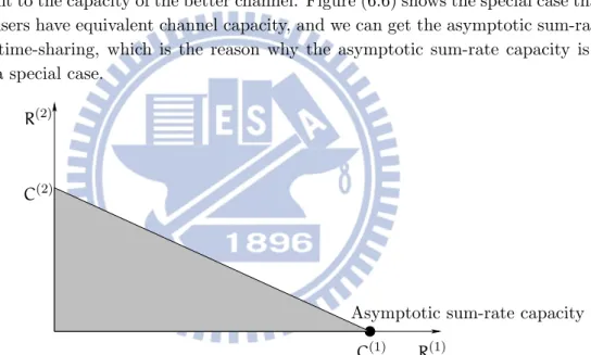
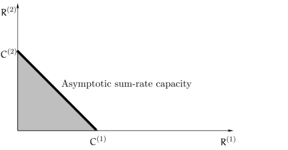
Actually, we also get the asymptotic capacity region of the multiple-access general fading channel at the same time. Because we need to reduce the multiple-user channel to the best single-user channel if we want to achieve the fading number, the asymptotic capacity is only one point in that region, not a line unless there are more than one user with best channels. Figure (6.5) shows the asymptotic capacity region in the case of m = 2. We can see all the possible rate pairs, and the asymptotic sum-rate capacity is a point in the figure, the value is just equivalent to the capacity of the better channel. Figure (6.6) shows the special case that both of the users have equivalent channel capacity, and we can get the asymptotic sum-rate capacity by time-sharing, which is the reason why the asymptotic sum-rate capacity is a line in such a special case.
R(1) R(2)
C(1) C(2)
Asymptotic sum-rate capacity
Figure 6.5: The capacity region of memoryless general fading MAC (2-user case).
In the case of m users with m > 2, as we mention in Section 3.1, the m-user capacity region is given by the convex closure of all rate m-tuples.
Possible future work for the multiple-access general fading channel might be as follows: • Considering the case with memory.
• Considering the case with side-information.
• Loosening the restriction that the receiver has only one antenna • Deriving the nonasymptotic capacity.
The first two point might be easier. We need to modify the channel model, considering the time index and the effects of feedback, to get the better capacity since both of memory
Chapter 6
R(1) R(2)
C(1) C(2)
Asymptotic sum-rate capacity
Figure 6.6: The capacity region of a special case: 2-user case with C(1)= C(2).
and side-information are helpful to our analysis. The difficulty in the third point is that we need to consider the more troublesome MIMO case, not only SISO and MISO cases. Finally, the last point is the hardest task since we do not know much about the o(1) term in equation (3.17). All the asymptotic tricks is not suited to this problem anymore, i.e., we need to restart from the upper and lower bounds to the nonasymptotic capacity of the fading channel.
Derivation of Equation (5.58) Appendix A
Appendix A
Derivation of Equation
(5.58)
Equation (5.58) holds only if we can prove the continuity of h(HTx) in x for all x are finite
and larger than 0. Here note that we prove for a general case with H is a nT× nR fading
matrix.
Let the sequence xn converge to x, !x! > 0. It then follows that the sequence Hxn
converges weakly to Hx. To simplify the notation, we let W = Hx, such that the sequence Wn converges weakly to W, i.e., Wn ⇒ W. Let the law of W be denoted by QW, the
law of Wn by QWn, the law of a zero-mean Gaussian random variable NC.0, E0WW†
1/ of convariance E0WW†1 by Q
W,G, and the law of a zero-mean Gaussian random variable
NC P 0, E 2 WnW†n 3Q of convariance E2WnW†n 3
by QWn,G. Then we obtain from the lower
semi-continuity of relative entropy in [2] that
lim n↑∞ D(QWn!QWn,G) ≥ D(QW!QW,G). (A.1) But D(QWn!QWn,G) = log(πe ) ν + log det E2W nW†n 3 − h(Wn), (A.2) and
D(QW!QW,G) = log(πe )ν + log det E
2
WW†3− h(W), (A.3)
Moreover, since E0WW†1 and E2W nW†n
3
is continuous, and determinants are polynomials of the corresponding matrix, we get log det E2WnW†n
3
−→ log det E0WW†1.
So we obtain lim n↑∞h(Wn) ≤ h(W), (A.4) i.e., lim n↑∞h(Hxn) ≤ h(Hx). (A.5)
Appendix A
It therefore remains to prove the reverse inequality lim
n↑∞
h(Hxn) ≥ h(Hx). (A.6)
Let ˜Z ∼ NC(0, InR) be independent of H. By choosing σ small enough, the following
inequality holds:
h(H + βσ ˜Z) − h(H) < ), (A.7) where β is an arbitrary number and is finite and larger than 0.
It now follows from (A.7) that for any xn, !xn! > 0,
h(Hxn+ σ ˜Z) − h(Hxn) = I(Hxn+ σ ˜Z; ˜Z) (A.8) = I D H xn !xn! + σ !xn! ˜ Z; ˜Z E (A.9) = I D P H+ σ !xn! ˜ ZQ xn !xn! ; ˜Z xn !xn! E (A.10) ≤ I D H+ σ !xn! ˜ Z; ˜Z E (A.11) < ), (A.12)
where the first inequality follows by the data processing theorem, because ˜ Z xn !xn! "−− ˜ Z"−− H + σ !xn! ˜ Z"−− P H+ σ !xn! ˜ Z Q xn !xn! (A.13)
forms a Markov chain, and where the last inequality follows from (A.7) with β = 'x1
n'.
By scaling properties of differential entropy, we are allowd to only consider the case that xhas unit length !x! = 1, i.e. x = ˆx. It now follows from (A.12) that for !xn! > 0,
h(Hxn) > h(Hxn+ σ ˜Z) − ) (A.14) = h(Hˆx+ H(xn− ˆx) + σ ˜Z) − ) (A.15) ≥ h(Hˆx+ H(xn− ˆx) + σ ˜Z 6 6H(xn− ˆx) + σ ˜Z) − ) (A.16) = h(Hˆx66H(xn− ˆx) + σ ˜Z) − ) (A.17) = h(Hˆx) − I(Hˆx; H(xn− ˆx) + σ ˜Z) − ), (A.18)
where the second inequality follows because conditioning cannot increase differential entropy. Expanding the mutual information term we obtain:
I(Hˆx; H(xn− ˆx) + σ ˜Z) = h(H(xn− ˆx) + σ ˜Z) − h(H(xn− ˆx) + σ ˜Z 6 6Hx)ˆ (A.19) ≤ nRlog ; E0!H!2 F 1 nR !xn− ˆx!2+ σ2 < − nRlog σ2. (A.20)
Here the inequality can be derived as follows. Firstly, note that since ˜Z is Gaussian and independent of H(xn− ˆx), we have h(H(xn− ˆx) + σ ˜Z 6 6Hˆx) ≥ h(H(xn− ˆx) + σ ˜Z 6 6Hˆx, H(xn− ˆx)) (A.21) = h(σ ˜Z) (A.22) = nRlog(πe σ2). (A.23)
Appendix A
Secondly, note that because among all random vectors of a given expected squared norm, differential entropy is maximized by the vector whose components are IID Gaussian. Hence, we get h(H(xn− ˆx) + σ ˜Z) ≤ nRlog πe E2!H(xn− ˆx) + σ ˜Z!2 3 nR (A.24) = nRlog ; πe.E0!H(xn− ˆx)!21 + nRσ2/ nR < (A.25) ≤ nRlog ; πe ; E0!H!2 F 1 nR !xn− ˆx! 2+ σ2 << . (A.26)
Inequalities (A.18) and (A.20) combine to prove that
lim
n↑∞h(Hxn) ≥ h(Hx) − ), (A.27)
and since ) > 0 is arbitrary, (A.6) is proven, which combines with (A.5) to prove the continuity of h(HTx) in x for all x with !x! > 0.
Derivation of Equation (5.72) Appendix B
Appendix B
Derivation of Equation
(5.72)
First, let an be a monotonical increasing unbounded sequence with n ↑ ∞,
and define fn(ˆx1)! E 4 log(|HT 1xˆ1|2+ m ' k=2 1 a2n!Hk! 2+ m ' j=2 2 an !H1!!Hj! + m ' i=2 m ' j=2 i)=j 1 a2 n !Hi!!Hj!) 5 − h(HT 1xˆ1), (B.1) f(ˆx1)! E0log |HT1xˆ1|21 − h(HT1xˆ1), (B.2) βn! sup 'ˆx1'=1 F|fn(ˆx1) − f (ˆx1)|G. (B.3)
Plugging (B.1), (B.2) into (B.3), we get
βn= sup 'ˆx1'=1 I6 6 6 6 6 E 4 log ; |HT 1ˆx1|2+ m ' k=2 1 a2 n !Hk!2+ m ' j=2 2 an !H1!!Hj! + m ' i=2 m ' j=2 i)=j 1 a2 n !Hi!!Hj! <5 − h(HT 1xˆ1) − E0log |HT 1xˆ1|21 + h(HT1xˆ1) 6 6 6 6 6 J (B.4) = sup 'ˆx1'=1 I E 4 log ; |HT 1xˆ1|2+ m ' k=2 1 a2 n !Hk!2+ m ' j=2 2 an !H1!!Hj! + m ' i=2 m ' j=2 i)=j 1 a2 n !Hi!!Hj! < − log |HT 1xˆ1|2 5J (B.5) = sup 'ˆx1'=1 I E 4 log ; 1 + 1 a2 n Om k=2!Hk!2 |HT 1xˆ1|2 + 2 an Om j=2!H1!!Hj! |HT 1xˆ1|2
Appendix B + 1 a2 n Om i=2 Om j=2 i)=j !Hi!!Hj! |HT 1xˆ1|2 <5J (B.6) ≤ E 4 log ; 1 + 1 an sup 'ˆx1'=1 I 1 an Om k=2!Hk!2 |HT 1xˆ1|2 + 2 Om j=2!H1!!Hj! |HT 1xˆ1|2 + 1 an Om i=2 Om j=2 i)=j !Hi!!Hj! |HT 1xˆ1|2 J5 (B.7) ≤ E 4 log ; 1 + 1 an sup 'ˆx1'=1 I Om k=2!Hk!2 |HT 1xˆ1|2 + 2 Om j=2!H1!!Hj! |HT 1xˆ1|2 + Om i=2 Om j=2 i)=j !Hi!!Hj! |HT 1ˆx1|2 J5 , (B.8)
where (B.8) follows because a1n ≤ 1. Hence lim an↑∞ βn≤ lim an↑∞ E 4 log ; 1 + 1 an sup 'ˆx1'=1 ;Om k=2!Hk!2 |HT 1xˆ1|2 + 2 Om j=2!H1!!Hj! |HT 1xˆ1|2 + Om i=2 Om j=2 i)=j !Hi!!Hj! |HT 1xˆ1|2 <5 (B.9) = E 4 lim an↑∞ log ; 1 + 1 an sup 'ˆx1'=1 ;Om k=2!Hk!2 |HT 1xˆ1|2 + 2 Om j=2!H1!!Hj! |HT 1xˆ1|2 + Om i=2 Om j=2 i)=j !Hi!!Hj! |HT 1xˆ1|2 <5 (B.10) = E[log(1)] (B.11) = 0, (B.12)
where in (B.10) follows from DCT.
Since limn↑∞an tends to infinity, this means that
E 4 log(|HT 1xˆ1|2+ m ' k=2 1 a2 n !Hk!2+ m ' j=2 2 an !H1!!Hj! + m ' i=2 m ' j=2 i)=j 1 a2 n !Hi!!Hj!) 5 − h(HT 1xˆ1) = E0log |HT 1ˆx1|21 − h(HT1xˆ1), (B.13) so equation (5.72) holds.