針對可靠的高畫質視訊傳輸的適應性技術

國立交通大學

電子工程學系電子研究所碩士班

碩 士 論 文

針對可靠的高畫質視訊傳輸的適應性技術

Adaptive Techniques for Reliable HD Video

Transmission

研 究 生：周禹伸

指導教授：黃經堯 博士

中 華 民 國 一百年三月

針對可靠的高畫質視訊傳輸的適應性技術

Adaptive Techniques for Reliable HD Video Transmission

研究生：周禹伸

Student：Yu-Shen Chou

指導教授：黃經堯

Advisor：Ching-Yao Huang

國 立 交 通 大 學

電子工程學系電子研究所碩士班

碩 士 論 文

A Thesis  Submitted to Department of Electronics Engineering & Institute of Electronics  College of Electrical and Computer Engineering  National Chiao Tung University  in Partial Fulfillment of the Requirements  for the Degree of  Master  in  Electronics Engineering  March 2011  Hsinchu, Taiwan, Republic of China  中華民國  一百年三月

  ‐ i ‐ 

針對可靠的高畫質視訊傳輸的適應性技術

學生：周禹伸 指導教授：黃經堯 博士

國立交通大學電子工程學系電子研究所碩士班

摘 要

重傳對於無線傳輸高畫質電視串流是很重要的，特別是強調於控制

每個

Video Frame 抵達的時間，避免延遲超過上限造成畫面無法即時解

碼。論文主要是對於即時高畫質電視傳輸提出一個

MAC 層系統架構及

演算法。我們不僅考慮了單一天線終端到終端的無線傳輸，也考慮了多

天線終端到終端的無線傳輸和多使用者多天線的無線傳輸。儘管文獻已

廣泛探討過最佳化

Throughput 的過程，但是對 Throughput 變化量的研

究則相對缺乏。我們考慮了平均的

Throughput 及 Throughput 的標準差，

來用以保證每個

Video Frame 能夠即時的到達接收端。為了達到上述目

的，此數學方法用來最小化每個

Video Frame 所需的傳輸時間，利用調

整

modulation coding scheme (MCS)以及每個封包的長度來滿足嚴謹

的

frame error rate 條件。每個 Video Frame 所需的傳輸時間定義為能夠

將一個

Video Frame 完全傳送到接收端(包含重傳)且滿足錯誤率條件的

最小時間。modulation coding scheme 以及每個封包的長度可以根據

即時的

SNR 和每個 Video Frame 的大小做動態的調整，MCS 的選擇及

封包長度的計算可完全被

MAC 層所決定用來做即時高畫質電視的無線

  ‐ ii ‐ 

frame 所需的時間，這些發現對於系統商建置無線傳輸即時高畫質電視

系統有很大的啟發。

  ‐ iii ‐ 

Adaptive Techniques for Reliable HD Video Transmission

Student：Yu-Shen Chou

Advisor：Dr. Ching-Yao Huang

Department of electronics Engineering

Institute of Electronics

National Chiao Tung University

ABSTRACT

 

Retransmission is necessary for the transmission of high-definition

(HD) video streaming. It is essential to control the arrival time of each frame

before the deadline. In this thesis, we present system architecture and a

related algorithm for real-time HD video transmission. The research focuses

on not only single antenna end-to-end wireless transmission but also

consider MIMO (Multi input multi output) end-to-end wireless transmission

and MU-MIMO (Multi-user MIMO) wireless transmission. While the

process of throughput optimization has been extensively investigated, the

variation of throughput is relatively unexplored. The average and variation

of throughput are considered together to guarantee the transmission of each

frame. For this purpose, the mathematical framework of this algorithm

minimizes the required transmission time under the strict frame error

constraint by adjusting payload length of each packet and modulation coding

scheme. The required transmission time is defined as a minimal period in

which the transmission could be completed and makes the error constraint

  ‐ iv ‐ 

satisfied. The parameters, payload length and modulation coding scheme,

can be adapted dynamically based on instant signal-to-noise ratio and the

data size of a video frame. This calculation can be completed punctually in

the MAC layer for the HD video transmission. The simulation result shows

that our proposed methodology can provide a quick, reliable way to

calculate the delay bound before transmission. These finding have

implications for operator developing a reliable wireless real-time HD video

system.

  ‐ v ‐ 

誌 謝

時間過的很快，轉眼間碩士畢業了，首先感謝我的父母對我的栽培以及無微不至的 照顧，讓我於求學階段不需為其他事情而煩惱，感謝老師  黃經堯教授在我碩士期間 的指導以及鼓勵，增進了我的信心，讓我快速的進入無線通訊領域並且更了解無限 通訊系統的知識及設計方法，讓我的研究內容能更趨完整與豐富。在對人生規劃及 一些未來方向，老師也常與我討論也給我適當的建議，讓我的視野更加寬廣。    謝謝在這段時間陪伴我一起成長的實驗室夥伴，有了你們的陪伴，更豐富了我的研 究生生活，希望在未來的生活能繼續互相勉勵，相互扶持，一起朝著目標理想努力。    2011 年  周禹伸撰 

  ‐ vi ‐ 

CONTENTS

摘 要 ... i  ABSTRACT ... iii  誌 謝 ... v  Contents ... vi  Figures ... vii  Table ... viii  Chapter 1  Introduction ... 1 

Chapter 2  System environment and architecture ... 4 

Chapter 3  Background On MIMO ... 7 

3.1  Single-user MIMO ... 7 

3.1.1  Spatial multiplexing ... 7 

3.2  Multi-user MIMO ... 9 

3.2.1  Zero forcing ... 9 

3.2.2  Block diagonal ... 11 

Chapter 4  Mathematical analysis and algorithm ... 14 

4.1  Minimal Required Transmission Time ... 14 

4.1.1  Single user transmission on wireless HD ... 14 

4.1.2  Single user MIMO transmission on wireless HD... 16 

4.1.3  Multi-user MIMO transmission on wireless HD ... 19 

4.2  Transformation of the optimization problem ... 21 

4.2.1  Single user transmission on wireless HD ... 21 

4.2.2  Single user MIMO transmission on wireless HD... 22 

4.2.3  Multi-user MIMO transmission on wireless HD ... 26 

4.3  Optimization framework ... 28 

4.3.1  Single user transmission on wireless HD ... 28 

4.3.2  Single user MIMO transmission on wireless HD... 29 

4.3.3  Multi-user MIMO transmission on wireless HD ... 30 

Chapter 5  Simulation result ... 31 

5.1  Simulation model and parameters ... 31 

5.2  Numerical result ... 33 

Chapter 6  CONCLUSION ... 44 

References ... 45     

  ‐ vii ‐ 

FIGURES

Figure 1: wireless real-time HD video service ... 1 

Figure 2: system model ... 5 

Figure 3: The system architecture of transmitter ... 6 

Figure 4: Parallel decomposition of single-user MIMO system ... 8 

Figure 5: The example of ZF precoding technique ... 10 

Figure 6: [7,(2,2,2)] MU-MIMO system to 6 parallel (2,1) MISO system ... 11 

Figure 7: The example of BD precoding technique ... 13 

Figure 8: [7,(2,2,2)] MU-MIMO system to 3 parallel (3,2) MIMO system ... 13 

Figure 9: The diagram of MAC packet with category 1 ... 18 

Figure 10: The diagram of MAC packet with category 2 ... 19 

Figure 11 The MRTT VS frame size (SISO case) ... 25 

Figure 12: WiMedia Standard PPDU structure ... 31 

Figure 13: Frame transaction analysis with Imm-ACK ... 32 

Figure 14 : Required transmission time versus SNR with D = 1Mb and Pe  10− 6 _{... 34}

  Figure 15 Link adaptation with Pe = 10− 6 _{... 34}

  Figure 16: Effective throughput and packet error rate versus SNR with D =1M ... 36 

Figure 17: PDF of required transmission time of a video frame at SNR=7dB... 37 

Figure 18: SNR VS. MRTT of received SNR=5dB (large scale) with SU-SISO system ... 39 

Figure 19: SNR VS. MRTT of received SNR=5dB (large scale) with SU-MIMO system ... 39 

Figure 20: SNR VS. MRTT of received SNR=10dB (large scale) with SU-MIMO system ... 40 

Figure 21: MRTT of single-user MIMO TDMA system VS. multi-user MIMOsystem with BD technique ... 41 

Figure 22: Indoor environment ... 42 

  ‐ viii ‐ 

TABLE

TABLE I PSDU rate-dependent Parameters ... 32 

TABLE II CONVOLUTIONAL CODE PARAMETERS ... 33 

TABLE III Cases of simulation ... 34 

TABLE IV LINK ADAPTATION THRESHOLD FOR MRTT ... 35 

TABLE V Our proposed algorithm VS. Optimal throughput alrorithm ... 37 

TABLE VI The fail rate corresponding to different SNR with different systems ... 40 

CHAPTER 1

INTRODUCTION

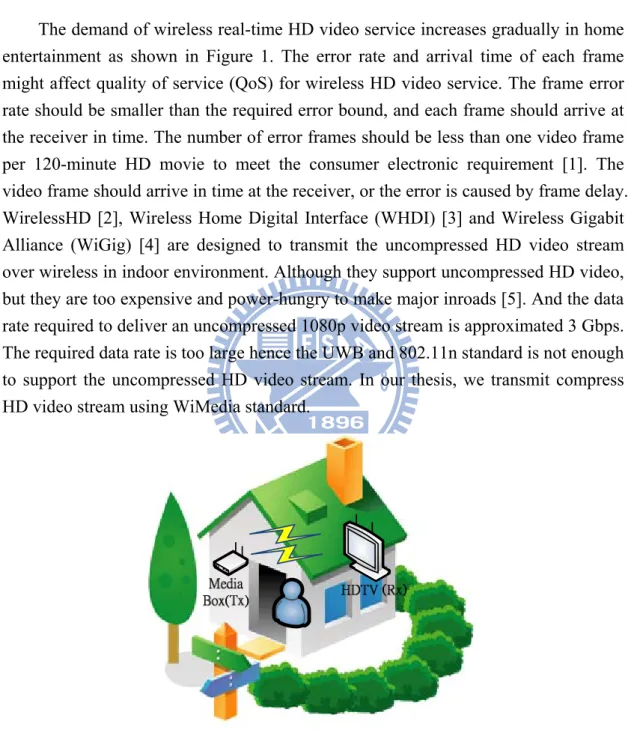
The demand of wireless real-time HD video service increases gradually in home entertainment as shown in Figure 1. The error rate and arrival time of each frame might affect quality of service (QoS) for wireless HD video service. The frame error rate should be smaller than the required error bound, and each frame should arrive at the receiver in time. The number of error frames should be less than one video frame per 120-minute HD movie to meet the consumer electronic requirement [1]. The video frame should arrive in time at the receiver, or the error is caused by frame delay. WirelessHD [2], Wireless Home Digital Interface (WHDI) [3] and Wireless Gigabit Alliance (WiGig) [4] are designed to transmit the uncompressed HD video stream over wireless in indoor environment. Although they support uncompressed HD video, but they are too expensive and power-hungry to make major inroads [5]. And the data rate required to deliver an uncompressed 1080p video stream is approximated 3 Gbps. The required data rate is too large hence the UWB and 802.11n standard is not enough to support the uncompressed HD video stream. In our thesis, we transmit compress HD video stream using WiMedia standard.

Figure 1: wireless real-time HD video service

In [6] [7] [8], the throughput has been improved and tried to reduce average arrival time of video frames. The payload length and modulation coding scheme (MCS) are adjusted based on the channel condition to maximize the effective data rate. These approaches satisfy the required throughput of video service. Throughput is the

average value of data rate, but the data size arriving at the receiver varies time by time. It could not guarantee whether the data of a frame arrives in time if the retransmission policy is allowed. The volatility of instantaneous throughput may cause the frame to delay, and an error may happen in the service. Sayantan takes the packet error rate into account in the throughput optimization problem in [9]. If the video frame is transmitted without retransmission, the arrival time could be predicted and controlled. The volatility of instantaneous throughput also becomes smaller. It provides better multimedia performance for lower resolution video without retransmission. For HD video service, the video frame error rate is usually hard to satisfy the consumer electronic requirement without retransmission, or the frame may delay caused by shorter payload length and large portion of overhead in a packet. As a result, the retransmission policy is required, and arrival time of each frame is also needed to consider in order to improve the quality of service. We should consider the volatility and average of throughput jointly.

The arrival time of each frame is tried to be controlled by estimating the required transmission time which makes the stringent frame error requirement satisfied in [10]. The required transmission time is defined as a minimal period in which the transmission could be completed and makes the error constraint satisfied. The authors use the payload length which maximizes the effective data rate and formulate a model to calculate the minimal required time based on the frame size. A look-up table is built to find the solution by interpolation method, because the problem is an integer programming problem and hard to solved punctually in the MAC layer. Interpolation errors would occur and make the solution away from the optimal value. The minimal required transmission time could be further reduced by adjusting payload length and MCS. For better performance, payload length and MCS should be also thought over, and an algorithm should be developed to solve the problem punctually in the MAC layer.

A joint optimization procedure and system architecture are provided to calculate the minimal required transmission time in this paper. The arrival time of each HD video frame could be controlled and further minimized under the constraint of stringent frame error rate with the retransmission policy. The required transmission time could be minimized by choosing proper payload length in MAC layer, MCS in physical layer based on the channel condition and frame size. The algorithm could solve the optimization problem easily and may be applied in MAC layer. This adaptive technique based on each frame size and channel condition might provide a reliable wireless HD multimedia service.

In order to increase coverage of video service and reach the strict frame error rate, MIMO systems is applied to maximize the throughput or reduce the packet error rate.

Since MIMO systems have been considered in recent years. One of the attractive features of MIMO systems is a multiplexing gain and consequently a higher spectral efficiency over single input single output (SISO) systems. According to the channel state information (CSI) feedback from the receiver to the transmitter. MIMO channel is decomposed into several parallel spatial channels by singular value decomposition (SVD). The required transmission time could be minimized by choosing proper payload length in MAC layer, MCS in physical layer based on each spatial channel and frame size, and power allocation on each spatial channel based on the channel condition. We investigate two categories to analysis the required transmission time using MIMO system. The first category assumes that the video frame is fragmented into packets with one optimal payload length, and each packet is encoded into symbols and transmitted between spatial channels. In other words, different spatial channel transmit symbols with different MCS. The second category assumes that the video frame is fragmented into packets with several optimal payload lengths. Each packet with different optimal payload length is mapped to different spatial channel according to its CSI. And every packet is divided into chips and transmitted using the specific spatial channel. That is to say, different payload length’s packet is transmitted by different spatial channel. And different spatial channel transmit symbols with different MCS. The results compare the performance of two categories and show that the first category gears towards multiplexing gain. It has no diversity gain. The second category yields both multiplexing gain and MAC-to-PHY diversity gain with a little complexity.

Among them is the minimal required transmission time (MRTT) issue which turns out to be severe when the resolution will get higher and the service coverage will get longer. In addition to that, from users’ point of view, we can notice that multi user transmission will be a leading technique in the future. To cope with these challenges, a two-step power-resource allocation algorithm has been designed to reduce the required transmission time of each user in this thesis. Here we apply two multiuser MIMO transmit preprocessing techniques for the downlink of multiuser MIMO systems. The techniques are block diagonalization (BD) and zero forcing (ZF) ,which decomposing a multiuser MIMO downlink channel into parallel independent single-user MIMO downlink channels. It has been shown that a significant reduction in multi-user MRTT algorithm than TDMA single-user MRTT algorithm when number of transmitted antenna larger than 4.

This paper is organized as follows. The system model is presented in next section. We will review the background on MIMO in CHAPTER3. An optimization problem is formulated and analyze in CHAPTER 4. The simulation results are discussed and shown in CHAPTER 5. Finally, we draw some concluding remarks in CHAPTER 6.

CHAPTER 2

SYSTEM ENVIRONMENT AND

ARCHITECTURE

In this chapter, we briefly describe the environment of wireless HD video transmission in indoor environments. The channel characteristic and properties of packet transmission are introduced. Besides, a cross-layer system architecture is constructed for these characteristics

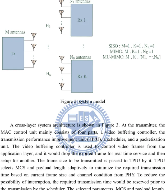
We mainly focus on a single interference-free architecture with K simultaneously active receivers (wireless HDTVs) served by one transmitter. The configuration of SISO, MIMO and multi-user MIMO systems are shown in Figure 2, where M antennas are located at the transmitter and Nk antennas are located at the kth receiver.

We assume that signal-to-noise ratio (SNR) is stable during the transmission time of a video frame [11]. The locations of the transmitter and receiver are mostly fixed for real-time HD video transmission in an indoor environment. We assume that the channel is flat fading and denote the MIMO channel to user k is Hk , which is a Nk *M

matrix. The (i,j) element of Hk is the complex gain from the ith transmit antenna at

the transmitter to the jth receive antenna at receiver. Its elements are independently identically distributed (i.i.d.) zero mean complex Gaussian random variables with unity variance. The multipath effect could be resolved by proper channel estimation techniques. Hence we suppose that channel state information (CSI) is known perfectly at both transmitter and receiver, the transmitter can adapt its transmission strategy relative to the channel. SNR is stable in this situation. However, SNR sometimes changes by people movement, and this shadowing effect influences SNR slowly.

SNR may change frame by frame. The packet success rate could be estimated by the values of SNR, payload length, and MCS [7][8]. During the transmission time of a video frame, the packet success rate is a constant if the payload length and MCS are selected. The events that the packet arrives at the receiver successfully are independent of each other, because each packet is received independently. As a result, the transmission of packets could be considered as a Bernoulli trial.

Figure 2: system model

 

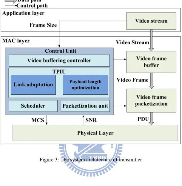
A cross-layer system architecture is shown in Figure 3. At the transmitter, the MAC control unit mainly consists of four parts, a video buffering controller, the transmission performance improvement unit (TPIU), a scheduler, and a packetization unit. The video buffering controller is used to control video frames from the application layer, and it would drop the expired frame for real-time service and then setup for another. The frame size to be transmitted is passed to TPIU by it. TPIU selects MCS and payload length adaptively to minimize the required transmission time based on current frame size and channel condition from PHY. To reduce the possibility of interruption, the required transmission time would be reserved prior to the transmission by the scheduler. The selected parameters, MCS and payload length, would be sent to PHY and the packetization unit. The frame is fragmented into packets by the chosen payload length, and then these packets is delivered to PHY and transmitted to the receiver by optimized MCS. At the receiver, each packet is received correctly in accordance with the order of transmission base on Imm-ACK mechanism. After the packets of a video frame are all received correctly, the video frame is aggregated and sent to the decoder to further process. If the frame is expired, the resource would be released to another transmission.

An optimization procedure is required in TPIU. It considers the payload length and MCS jointly based on the frame size and channel condition. The mathematical analysis and algorithm for this procedure will be investigated in the following chapter.

CHAPTER 3

BACKGROUND ON MIMO

  Multiple antennas at the transmitter and receiver of a wireless communication system can increase data rates and performance. In this chapter we provide an overview of the parallel decomposition on MIMO channel of single-user and multiuser MIMO channels. This chapter starts with models that were developed in an attempt to describe precoding techniques for multiplexing gain and interference cancelation applications for MU-MIMO. Applying these techniques, we reduce the complexity and provide a simple system model to analyze TPIU in next chapter.   

3.1 Single­user MIMO 

  MIMO systems are defined as point-to-point communication links with multiple antennas at both the transmitter and receiver. In particular, recent research has shown that MIMO systems can significantly increase the data rates of wireless systems without increasing transmit power or bandwidth. The cost of this increased rate is the added cost of deploying multiple antennas, the space requirements of these extra antennas and the added complexity required for multi-dimensional signal processing

[11] .

3.1.1

Spatial multiplexing

  In this section we focus on the precoding techniques to enhance the spatial multiplexing gain of single-user MIMO channels. We consider the perfect channel state information at the transmitter during this thesis. The system model is shown in Figure 2 and assume number of receivers K=1. The received signal y of the single user MIMO system can now be expressed by the following equation:

Where y is an N1-by-1 vector and x is the M-by-1 transmitter signal vector. H

represents the flat-fading channel matrix. And n is the i.i.d, unit-variance, additive Gaussian noise vector at the receiver.

  With perfect CSI at transmitter, the flat fading channel matrix H is assumed to be known at the transmitter and receiver. Applying singular value decomposition (SVD) to H, we can express it as

H can be broken down into the product of three matrices - an orthogonal matrix U, a

diagonal matrix D, and the transpose of an orthogonal matrix V. Where  , ; the columns of U are orthonormal spatialvectors of HHT , the columns of V are orthonormal spatialvectors of HT_{H, and D is a diagonal matrix containing the}

square roots of spatialvalues from U or V in descending order. Replacing (2) into (1), we obtain

Where ́ , ́ , ́ . Note that the channel matrix H has been decomposed into rank(H)=m≦min(M, N1) parallel spatial subchannels since D is

diagonal.

An important result of the SVD precoding technique show that the single user MIMO system is than transformed into m parallel SISO system. The parallel SISO system is shown in Figure 4. Where λi is i-th diagonal element of D.

1 λ 2 λ m

λ

 

Figure 4: Parallel decomposition of single-user MIMO system

  SVD technique make a significant contribution to analyze the subchannel power gain easily; hence the received SNR at each spatial channel can be derived. According to the received SNR at each spatial channel and using SVD, the optimization procedure to calculate the minimal required transmission time by adapting the MCSs and payload length will be investigated in next chapter.

  (2)

3.2 Multi­user MIMO 

  Multi-user MIMO has recently emerged to be a leading next-generation-network technology. There has been considerable recent interest in Multi-user MIMO communication due to their potential for dramatic gains in channel capacity. Multiuser MIMO techniques have several key advantages over single user MIMO communications [12]. Research in this area has focused on throughput maximization. However, there still has multi-user interference and multi-antenna interference degraded the throughput. The goal of this article is to provide a method minimizing the required transmission time base on instaneous channel condition (SNR) for wireless HD and guarantee the QoS for each user. For simplicity, linear precoding technique will be applied to overcome interference and measured the received SNR. And the multi-user MIMO system will be transformed to multiple single user MIMO systems. In this way, the MRTT will be investigated in next chapter. The rest of this chapter will introduce two linear precoding techniques, which are zero forcing (ZF) and block diagonal (BD).

3.2.1

Zero forcing

  In this section, we introduce the system model and briefly account the zero forcing method for multiuser MIMO systems presented in [13]. The configuration of multi-user MIMO system is shown in Figure 2:  system  model Considering the scenario that , denote the transmit symbol at i-th antenna for user n, and , denote the additive white Gaussian noise symbol at i-th antenna for user k. The received symbol at -th antenna for k-th user can be express as: 

Where , _{is 1 *M flat fading channel matrix at -th antenna for user k and} , _{is M *1 precoding matrix at transmitter corresponding to i-th antenna for user n.} The principle aim of zero forcing technique is to design ,

… ; … such that all multi-user interference and multi-antenna interference are zero. In this view,

, , _{0          . In other words, it can be shown that} the solution is equivalent to equitation (5).

, ₌ , _{∑ ∑} , , ,   ₍₄₎

Here we let , , , , and choose , is a matrix that contacting all spatial vectors of , … , _… ,

 &  corresponding to zero spatial value. Also choosing , is contacting all non-zero spatial vectors of , , and , is the corresponding vectors have all singular values. There is still limitation on number of transmitted antennas ∑ ∑ 1 1. Because there should exist at least one spatial vector which is null space of

, _… , _… ,

 &  .  Also  ,  is a  ∑ ∑ 1 1    by one vector. Replacing this to equation (4), we can rewrite the equation (4) as equation (6) and the precoding method shown in Figure 5 as example.

 

Figure 5: The example of ZF precoding technique , ₌ , , , ,  

      = , , , , ,   ₌ , , ,  

After multiplying precoding matrix , ,  the received symbol can be written as general Single-user multi-input single-output (MISO) case. By estimating channel matrix H and applying the ZF technique, the received SNR at i-th antenna for user k could be estimated. Therefore, the [M,K*N] multi-user MIMO system can be simplified to KN parallel (M − (KN-1)) × 1 single-user MISO system. Figure 6 shows the example of zero forcing technique with [7,(2,2,2)] multi-user system transformed to 6 parallel (2,1) single-user MISO system. [7,(2,2,2)] multi-user system denote a system have 1 transmitter with 7 transmit antennas and 3 receivers with 2 antennas each.

 

Figure 6: [7,(2,2,2)] MU-MIMO system to 6 parallel (2,1) MISO system

 

3.2.2

Block diagonal

  This section outlines a procedure for finding the optimal precoding matrix such that all multi-user interference is zero  [14]. Reference to Figure 2, In a downlink multiuser MIMO system with K users, which is so called the (M,KN) multi-user system. The transmitted symbol of user i is denoted as a R -dimensional vector , which is multiplied by a N × R precoding matrix and sent to the basestation antenna array, the received signal for user k can be represented as

The interference is seen by other user’s signal to user k, and is AWGN noise with 0,1 . To eliminate the multi-user interference, the key role of block diagonal is to precode each user’s data with precoding matrix , such that

is unitary matrix and

If we define as:

In order to satisfy the constraint in (8), shall be the null space of . Here we set , and choose is a matrix that contacting all spatial vectors of

corresponding to zero spatial value. Let Pi represents the rank of .

interprets the equivalent single-user MIMO channel. Applying singular value decomposition (SVD) to , we can express it as

Choosing equal to  , the received signal for user k after BD precoding technique can be represented as:

There is still limitation on number of transmitted antennas 1 . Because there should exist at least one spatial vector which is null space of

.  Also   is a  1  by one vector. The BD precoding method is shown in Figure 7 as example. 0      & 1 ,   (8) = … … T ₍₉₎   (10) ́ = ∑           = ∑           =           =           =           =   (11)

 

Figure 7: The example of BD precoding technique

After BD precoding technique, the received symbol can be written as general Single-user multi-input single-output (MIMO) case. By estimating channel matrix H and applying the BD technique, the received SNR at i-th antenna for user k could be estimated. Therefore, the [M,K*N] multi-user MIMO system can be reduced to K parallel (M − K (N-1)) × 1 single-user MIMO system. Figure 8 shows the BD technique with [7,(2,2,2)] multi-user system transformed to 3 parallel (3,2) single-user MIMO system.

…

CHAPTER 4

MATHEMATICAL ANALYSIS AND

ALGORITHM

In order to achieve the video frame error criterion with insufficiently large packet success rate, the retransmission mechanism is then the conventional solution but at the cost of the extra delay. As to reduce the possibility of interruption in the transmission process, the required transmission time would be reserved prior to the transmission by the scheduler. The following parts in this subsection, we will define the optimization problem of MRTT base on single user, single-user MIMO and multi-user MIMO systems. And provide a relatively comprehensive analysis the impact of payload length, modulation coding scheme on required transmission time, and then we will solve the optimization problem. Finally, the optimization framework will be addressed.

4.1 Minimal Required Transmission Time 

In this subsection, we formulate a mathematical model for the analysis of the minimum required transmission time for HD video transmission.

4.1.1

Single user transmission on wireless HD

Suppose that a video frame is fragmented into NF packets with a fixed payload

length L bytes. We reserve a period for the transmission in which more packets than the fragments could be transmitted. If the transmission of these fragmented packets could be completed during the reserved time, the frame transmission succeeds. The transmission time may shorter than the reservation, and the remaining time could be released for other transmission. Since the transmission of these packets is a Bernoulli trial in this period, the error rate Per that the frame is not able to arrive at receiver is

where P() is the packet success rate (PSR), γs is SNR, m is the mode of MCS, and NR

is the number of packet which could be accommodated in the reserved period. , , 1 , , (12)

Considering all possible transmission paths with the retransmission policy, we can regard the reserved period as a bound to reach the error constraint Per.

  The required transmission time is defined as a minimal period in which the transmission of a frame could be completed and makes the error constraint satisfied. It could be minimized by adapting payload length and MCS to the channel condition and frame size. The joint optimization problem is formulated as

,      ,   subject to  , , 1 , ,   8   0  (13) 

where D and T() represent the data size of a video frame in bits and the transmission time of a packet respectively, and Pe is the target frame error rate. This optimization

problem still involves the integer programming, and its complexity should be reduced further.

In order to solve the optimization problem (13), we would like to transform it into an explicit form in terms of L and m. The constraint should be also modified to reduce the complexity. First, P and T are replaced by the functions in terms of L and

m, and then we modify the frame error constraint. We estimate PSR of two cases. One

is the transmission with only modulation, and the other is the transmission with the convolution code and modulation. The packet success rate can be formulated as [16][17]:

, , 1

1  

(14) where b is bits per symbol in modulation, PM( ) is symbol error probability of

M-QAM, and   is union bound of first event error probability corresponding to PHY-mode m for coded situation. and could be calculated based on the channel condition γs and PHY-mode m according to the equations from [16] and

, 8 (15)

where is total overhead of a packet in PHY-mode m including acknowledgment, either positive (ACK) or negative (NACK), and other redundancy, and R(m) is transmission rate corresponding to PHY-mode m in bits per second.

4.1.2

Single user MIMO transmission on wireless HD

In this subsection we focus on the analyzing the MRTT of single-user MIMO channels. We would provide two mathematical models to analyze TPIU. In these two category, we will applied SVD precoding technique to precode the transmitted data and measure the current channel condition. The single-user MIMO system will transform to equivalent non-interfering single-user SISO system. Without lose of generality, we suggest single-user 2-by-2 MIMO system during this formulation.

With category 1, to optimize the transmission performance of HD video, TPIU

selects MCSs and payload length adaptively to minimize the required transmission time based on current frame size and channel conditions from PHY. The reference stack design is shown in Figure 3 and Figure 9. At the transmitter, the video frame is fragmented into packets by the optimal payload length L, and then these packets is delivered to PHY and transmitted to the receiver by optimized MCSs. With current SNR of each equivalent SISO channel, the TPIU unit will encoded the packet into chips and modulated to symbols with two types. These two type of symbols than sent to the precoding matrix. Finally, the spatial channel 1 will transmit the symbol with

C1, R1 and M1 and the spatial channel 2 will transmit the symbol with C2, R2 and M2.

Where Ck, Rk and Mk are represent the code rate, data rate and modulated chip per

symbol with spatial channel k. Since the packet is encoded and modulated with two types, the packet success rate can be formulated as:

 ,  , 1 1 ((16)

Where   represents the symbol error probability PM( ) of M-QAM and union

bound of first event error probability corresponding to PHY-mode m for coded situation   .  represents the current SNR of equivalent SISO channel k. Lk is

the equivalent payload length in a packet with Ck, Mk. The minimum required

transmission time is occurred when each spatial channel has the same transmission time. Hence L1 and L2 can be formulated as:

1

2

=>

1

2

(17)

Substituting the equation ((17) into equation ((16), the packet success rate can be represented as:

Reference to equation (13), the MRTT of single-user 2-by-2 MIMO system can be written as: , ,      , ,   subject to   ,  , 1  ,  ,   8   , , 8 1 2   0  (19) 

Where is total overhead of a packet in time. T() represent the transmission time of a packet according to , , . In this problem, the goal is choosing the optimal payload length and MCSs that achieving the MRTT. And we will solve the problem in next section.

leng MC time con into k pa sym refe cate Hen chan m , subj  1  1 1 In contrar gth Lk to th CSs and mul e based on sidering sin o two types acket will e mbol, then s erence diagr egory 2, eac nce we focu nnel. The op min , , max ject to       ∑ ∑     8 Figure 9: T ry to catego he equivale ltiple paylo current fra ngle-user 2-which are w encoded int sent to the ram is show ch type of us on minim ptimization C C The diagram ory 1, the ca nt SISO sp oad length a ame size an -by-2 MIMO with optima o chip with precoding wn in Figure packet is tr mize the ma n problem ca , ,  ,  , 8   m of MAC p ategory 2 tr patial chann adaptively t nd channel O system, t al payload le h code rate matrix corr e 3 and Figu ransmitted aximal requ an be formu 1 1 packet with ansmits pac nel k before to minimize conditions the video fr ength L1 and Ck and mo responding ure 10. For t to the spati uired transm ulated as equ ,  ,  , category 1 ckets with o e precoding e the require from PHY ame will di d L2 respect odulated wit to spatial the MRTT c ial channel mission tim uation (20).     optimal pay g. TPIU sel ed transmis Y. For insta ivide the pa tively. The th Mk chips channel k. calculation independen me of the sp . (20)  yload lects ssion ance, acket type s per The with ntly. patial

, Wh con Bern succ And divi que

4.1

Mul The the form  , 1, 8 8 ,  0 

ere the vid straint. Sin noulli trial cess rate tha d there still ides by num stion (20) in

.3

Mul

Applying lti-user MIM erefore, the maximal tr mulated as: 1 8 1 8 deo frame e nce the tran in this peri at all packet l another q mber of typ n next secti   Figure 10:

lti-user M

the ZF prec MO system objective is ansmission 1  1 , , ₂, 0  error rate co nsmission o iod, so the f ts transmitt question tha pe 2 packet on. The diagram

MIMO tra

coding tech m will transf s that guaran time of the  , 8 onstraint is of these pac frame succe ted with spe

at the prop ts should b m of MAC

ansmissio

hnique or BD form to mu ntee the Qo e SISO chan 1 2 transform ckets with ess rate is m ecific spatia portion of n be derived. packet with

on on wir

D precoding ultiple equiv S of all user nnel pair, th 2  2     to the fram each spatia multiply all al channel ar number of And we w   h category 2

reless HD

g with SVD valent SISO rs, so we w he MRTT al me success al channel spatial cha rrive at rece type 1 pac will simplify 2

D

D technique O channel p ant to minim lgorithm ca rate is a annel eiver. ckets y the , the pairs. mize an be

Minimize      max _{, , , ,} , _, , 1, … , 1, …   subject to        1 ∑   , , _, , , , , , _{1   ,} , , , , , …  1 ∑   , , _, ,  , , , , _{1   ,} ,  , , , , 1       ,k=1,…,K  , , 8 ,  , 1, … ,     , ,  , , 1 ,   , _{, 1, … , 1, …}   , , 8 , 0, 1, … , 1, …   , 0, 1, … , 1, …   (21) 

Where k and n represent the receiver number and spatial channel number respectively. The video frame success rate constraint should be reached of each user. And each spatial channel transmits the symbol with best PHY-mode and the packet with optimal payload length to minimize the required transmission time. Compares in single-user MIMO system, we must guarantee the QoS for each user, hence the water filling method is not suitable for multi-user application. Joint design the power allocation scheme and resource allocation per antenna base maintain the QoS constraint and provide higher resource utilization efficiency.

4.2 Transformation of the optimization problem 

4.2.1

Single user transmission on wireless HD

To simplify the frame error constraint, we would like to express NR as a function

in terms of NF, , , , and Pe. The left side of frame error constraint is a

cumulative distribution function (CDF) of binomial distribution, and it could be approximated by a CDF of standard normal distribution provided by Molenaar (1970a) [15]. The first constraint in (13) becomes

4 1 . _{1 , ,} . _{4 4}

30.5 , , 0.5     (22)

whereΦ is the CDF of standard normal distribution. If we reserve more time, the error rate becomes lower. In other words, the required time becomes shorter if the error rate approaches Pe. As a result, the required time reaches optimum in (13) when

the constraint is equal to the target frame error rate Pe. The constraint is rewritten as

4 1 . _{1 , ,} . _{4 4}

30.5 , , 0.5     (23)

Where Φ e = Pe. Φ is a one-to-one function, so the inputs is identical in both

sides of (23). We can solve the equality and get the equation

1 4 1 1 , , 4 , ,

1 4

(24)

Combining (13) (14) (15), and (24), we transform the original problem (13) into 

   8 1 4 ₈ 1 1 1 4 1 1 4 8            0  (25)

where p represents the symbol error probability in the uncoded case or the union bound of the first-event error probability in the coded case, and C is 8/b or 8 for the uncoded case or the coded one respectively.

4.2.2

Single user MIMO transmission on wireless HD

Considering category 1, the MRTT can be written as (19), the simplify method is similar to 4.2.1. Replacing the binomial CDF by a normal approximation, and the frame error rate is reached the target frame error rate Pe, we transform the original

problem (19) into , ,      , ,     1                          0 (26) Where Φ e = Pe.

Taking into account of category 2, let us define the spatial channel success rates as (1- Pe1) and (1- Pe2). The frame success rate constraint can be written as 1

1 1 . Since the frame error rate is very small, we can see that . With a change of variables, let us set 0.5 . Therefore, the frame success rate constraint can be transform into two independent frame error rate constraints. i.e.:

  C  , 1 ,

  C  , 1  , (27)

Applying the normal approximation by Molenaar (1970a), the number of packet which could be accommodated in the reserved period  and  can be replaced as:

1 4 1 1 1   4 1   1 4 1 4 1 1 1   4 1 1 4   (28)

Where Φ e = 0.5 Pe. Combining ((28), we can convert the optimization problem

(20) as:     T =  ,   ,   1 4 1 1 1   4 1   1 4 1 4 1 1 1   4 1   1 4   8 8   8 ,  8 0  ,    , 0  (29)

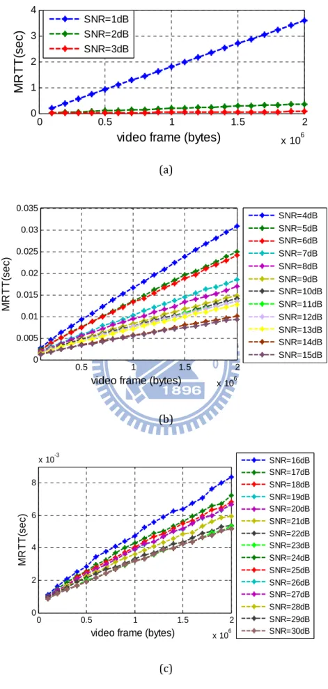
It can be verified that the objective function is occurred when the required transmission time of two spatial channel are equal. In order to solve this problem, we need to divide the video frame into two parts, and . By simulation, we can see that the video frame size is approximated linear with MRTT in Figure 11. Hence for fixed SNR , using least square method, we can built up a table contain parameters _,  and  _, . Consequently, by table look up, the transmitted frame size of equivalent SISO channel pairs are:

 

  , , ,

, ,  

Where  denote the MRTT of . is the transmitted equivalent video frame size of spatial channel corresponding to . ,  and  , are the least square parameters of . After replaced these variables by the function of L and applied the equation ((30), the optimization problem is defined as:

T = Max( , Min ₈1 1 1 4 1 1 1 1 1   1 2 4 1   1 1 4 8₁ 1     , , , , , 0  0    ₂ 1     2         0    0  (31)

Note that the optimization problem in the above form converted to two independent optimization problems, like the single-user SISO system. And the MRTT of MIMO system is the maximum one of each spatial channel.

  (a)    (b)    (c) 

Figure 11 The MRTT VS frame size (SISO case)

0 0.5 1 1.5 2 x 106 0 1 2 3 4

video frame (bytes)

M R TT( s e c ) SNR=1dB SNR=2dB SNR=3dB 0.5 1 1.5 2 x 106 0 0.005 0.01 0.015 0.02 0.025 0.03 0.035

video frame (bytes)

M R T T (se c) SNR=4dB SNR=5dB SNR=6dB SNR=7dB SNR=8dB SNR=9dB SNR=10dB SNR=11dB SNR=12dB SNR=13dB SNR=14dB SNR=15dB 0 0.5 1 1.5 2 x 106 0 2 4 6 8 x 10-3

video frame (bytes)

MR T T (s e c ) SNR=16dB SNR=17dB SNR=18dB SNR=19dB SNR=20dB SNR=21dB SNR=22dB SNR=23dB SNR=24dB SNR=25dB SNR=26dB SNR=27dB SNR=28dB SNR=29dB SNR=30dB

4.2.3

Multi-user MIMO transmission on wireless HD

In order to solve the QoS provisioning problem for all users, we introduce a efficient power allocation method. Since the transmitter and receiver are fixed in indoor environment, without considering fading gain, the power received from transmitter at receiver i is given by

    ,  1, …  

 

0  1, …

 

(32)

The nonnegative number represents the path gain from the transmitter to the i th receiver. can encompass path loss, shadowing, antenna gain, coding gain, and other factors. denotes the power transmitted from transmitter to receiver i.

 represents the total transmitted power.

Our power allocation method is shown below. First, we let all user has same receive power,  ,  2, … . This method solve the location problem, it can allocated more power on some user that far from transmitter. It secures some outage users. Second, we apply optimal power allocation for each user. The optimal power allocation in this case is a“water-filling” and shown below, where power and data rate are increased when channel conditions are favorable and decreased when channel conditions are not favorable.

,   0, , ,

 

,

 

(33)

By table look up method similar to category 2, the equivalent frame size of each spatial channel with each user is given by

, , , , , , , , ,   , , , , , , , , ,   1 , 0 0 1 , , 0 1 0 , … … … … , 1 0 0 , , , , , , , ,   , ,

 

(34)

Where _, denote the SNR of spatial channel n with user k. _,  denote the MRTT of _, . _, is the transmitted equivalent video frame size of spatial channel corresponding to _, . _{, ,}  and  _{, ,} are the least square parameters of _, . Finally, applying power allocation method, and table look up method, the equation ((21) is transform into optimal MRTT of each spatial channel pair, and the MRTT of the multi-user system is maximum MRTT of all spatial channel pairs.

T = Max( _,  , 1, … , 1, … , , 8 , 1 4 _, , 1 1 1 ,   , 4 1 ,   , 1 4 8 , , , , , , 0    e 1/

 

(35)

4.3 Optimization framework 

4.3.1

Single user transmission on wireless HD

To find the payload length and MCS that minimize the required transmission time, we use two-step procedure to solve (25). In the first step, we fix each PHY-mode m and calculate the optimal payload length and minimal required transmission time in each mode. Second, we choose the minimum of transmission time among these PHY-modes.

Fixing m, we use Newton's method to find the optimal length L*. Since objective function is a convex function of L, we can calculate the optimal length L* by first-order differentiation of the objective function and then apply Newton’s method to find its root. The root is the optimal length. Newton’s method is one of the most useful methods for finding successively better approximations to the roots of a real-valued function, and Newton’s method can converge quickly. In our case, it converges at most six iterations if the initial guess of L is set to be zero. It can be accelerated by choosing proper initial value. The algorithm of Newton’s method is summarized as follows: Step 1: Let f(L) be the object function in (25). The derivative of f is zero at the minimum, so the minima can be found by applying Newton's method to the derivative. Set a initial guess L( ), and use the iteration given by

f′

f" (36)

where f ‘( )and f ”( ) are the first and second derivatives of f respectively. The iterative procedure stops when Ln+1- Ln is less than the specified tolerance. We can get the

optimal payload length in each PHY-mode, and then the best PHY-mode could be determined by selecting the minimal required time among the PHY-modes. In practice, the optimal PHY-mode under different channel conditions is built into a table, and the payload length is the only variable for the optimization problem (25).

A mathematical model is formulated to minimize the required transmission time based on the channel condition and frame size. The optimal joint adaptation of payload length and MCS could be obtained by solving it. The detail of the algorithm operated in TPIU is as follows:

Step2: Choose the optimal PHY-mode m based on γs.

Step3: Determine the C, , and R(m) according to m. Step4: Calculate the error probability p based on m and γs.

Step5: Use Newton's method to get L*. Step6: Determine the minimal required transmission time.

4.3.2

Single user MIMO transmission on wireless HD

Similar to single-user SISO case, by looking up the table, the optimal PHY-mode is choose under different channel conditions. And applying the Newton's method to find the optimal payload length in (26) ((31) for different categories, the detail of the algorithm operated in TPIU is as follows:

Category 1:

Step1: Report channel condition and measure the current video frame size (D).

Step2: Using SVD technique and applying water-filling power allocation, then report current SNR (γs ) on each equivalent SISO channel pair.

Step3: Choose the optimal PHY-mode m based on each γs .

Step4: Determine the C, Ot (m) ,and R(m) according to each PHY-mode m.

Step5: Calculate the error probability p based on each m and γs.

Step6: Use Newton’s method to get L . Step7: Determine the MRTT.

Category 2:

Step1: Report channel condition and measure the current video frame size (D).

Step2: Using SVD technique and applying water-filling power allocation, then report current SNR (γs ) on each equivalent SISO channel pair.

Step3: Using the lookup table to calculate the transmitted equivalent video frame size         1 and for each spatial channel.

Step4: Choose the optimal PHY-mode m based on each γs .

Step5: Determine the C, Ot (m) ,and R(m) according to each PHY-mode m.

Step6: Calculate the error probability p based on each m and γs.

Step7: Use Newton’s method to get optimal payload length corresponding to each spatial channel.

Step8: Determine the MRTT of each spatial channel and choose the maximal one be the MRTT of single-user MIMO system.

   

4.3.3

Multi-user MIMO transmission on wireless HD

The MRTT algorithm is a standardized measure designed to predict the minimum required transmission time of wireless HD video system. Applying precoding technique and power allocation method, we can choose the best PHY-mode

m and the corresponding optimal length to minimize the required transmission time of

each equivalent SISO channel pair for high quality HD video transmission. The detail of the algorithm operated in TPIU is summarized below:

Step1: Report channel condition and measure the current video frame size (Dk) that

will transmit to receiver k.

Step2: Using the lookup table to calculate the transmitted equivalent video frame size for each spatial channel.

Step3: Using ZF or BD precoding technique and proposed power allocation method, then calculate current SNR (γs ) on each spatial channel.

Step4: Choose the optimal PHY-mode m based on each γs .

Step5: Determine the C, Ot (m) ,and R(m) according to each PHY-mode m.

Step6: Calculate the error probability p based on each m and γs.

Step7: Use Newton’s method to get optimal payload length corresponding to each spatial channel.

Step8: Determine the MRTT for each spatial channel and choose the maximal one be the MRTT of the multi-user MIMO system.

CHAPTER 5

SIMULATION RESULT

WiMedia transmission protocol will be used as the simulation platform in this paper. WiMedia standard specifies the ultra wideband (UWB) for a high-speed, short-range wireless network, and HD multimedia service could be operated over it. The same procedure could be also applied to other systems with capability to transmitting HD videos.

5.1 Simulation model and parameters 

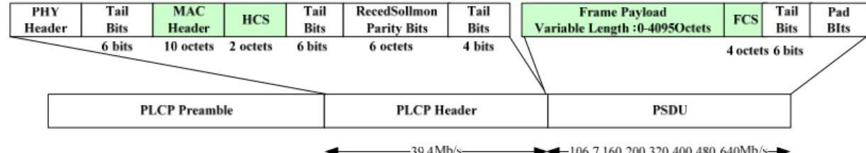
The system parameters are listed in TABLE I. Seven PHY modes are provided with different modulation and convolution coding schemes for link adaptation. We also include the case without channel coding, because the uncoded case will get better performance rather than coded case in high SNR range. The details of these parameters can be referred to [10] and [18]. The packet in WiMedia is called the physical protocol data unit (PPDU) composed of three components: the PLCP preamble, the PLCP header, and the physical service data unit (PSDU) have shown in Figure 12. The interval of PLCP preamble is 9.375us for Immediate Acknowledgement (Imm-ACK) policy. The PLCP header must be sent at a lower data rate of 39.4Mb/s to guarantee the correctness. The PSDU can be sent at the data rate chosen from TABLE I due to different PHY-mode. The length of PLCP Header mainly composed of PHY header, MAC header, and header check sequence (HCS) is 26 bytes. The length of PSDU varies according to the frame payload length from 0 to 4095 bytes. Because of we need to simulate the impact of the payload length on reservation time, so the payload length is not constraint in this thesis.

The overhead in each packet transmission contains two parts, the cost of retransmission and the necessary control information of different MAC format in a packet. The detail of transmission mechanism with Immediate Acknowledgement (Imm-ACK) policy during the reservation time is shown in Figure 13. The receiver should respond with an Imm-ACK frame after a period of Short Interfarme Space (SIFS) for each packet transmission. To derive the first event error probability, the weight spectral of the punctured convolutional code has been computed in [19]. TABLE II shows the code rate corresponding to the free distance weight spectral, and generator polynomials. Forward error correction (FEC) is performed by rate-1/3 convolutional coding. The higher code rates of 1/2, 5/8 and 3/4 are obtained by puncturing the original rate-1/2 code, and the constraint length is 7. The packet error rate could be calculated from these parameters. In the case of HD videos, the video frame size of HD video is from 0.3 to 3 Mb with about 45 dB PSNR [20]. Without loss of generality, we assume the video frame size is equal to 1 M bits and the frame rate of video is 30 frame per seconds in the following simulation. The corresponding constraint of transmission delay is 1/30 second. Due to the limited buffer size at decoder, we consider the situation that the first video frame arrives at the receiver and then the decoder starts the decoding procedure.

Figure 13: Frame transaction analysis with Imm-ACK

TABLE I

PSDU rate-dependent Parameters

PHY mode R (Mbps) Modulation Code Rate Ot (μs)

Mode 1 106.7 QPSK 1/3 50.48 Mode 2 160 QPSK 1/2 50.36 Mode 3 200 QPSK 5/8 50.31 Mode 4 320 DCM 1/2 50.24 Mode 5 400 DCM 5/8 50.22

Mode 6 480 DCM 3/4 50.20 Mode 7 640 DCM Without coding 50.18

TABLE II 

CONVOLUTIONAL CODE PARAMETERS 

Code rate Generators dfree _{ad; d   df; df 1; : : : ; df  19}  

1/3 133, 165,171 15 3, 3, 6, 9, 4, 18, 35, 45, 77, 153, 263, 436, 764, 1209, 2046, 3550,  5899, 10002,16870, 28701   1/2 133,171 10 11, 0, 38, 0, 193, 0, 1331, 0, 7275, 0, 40406, 0, 234969, 0,  1337714, 0, 7594819, 0,43375588, 0 5/8 133, 165,171 6 _{1,19,71,168,546,2004,6391,21431,71709,235868,0 … 0} 3/4 133, 165,171 5 4,36,175,882,4486,23156,120602,622937,3216664,1662899,0 …  0  

5.2 Numerical result 

Figure 14 shows the variation of required transmission time with different SNR, and the related description of each case is listed in

TABLE III. The required transmission time of each approach is selected from the best mode in TABLE I. The discontinuity of each curve is caused by the mode adaptation to the shortest required transmission time. The real optimal solution to the integer programming problem (13) is close to minimal required transmission time (MRTT) solved from (25). The original problem is converted into another with lower complexity by the normal approximation (23), and it still retains a good accurate solution. We could get the payload length and required transmission time in each mode within six iterations using Newton‘s method in our simulation result when the initial value L() is set to be 1 byte. TABLE IV is the best PHY-mode of MRTT in different SNR regions, and the details of adaptation are shown in Figure 15. We could select the best PHY-mode based on instant SNR by this table. The computation complexity in MAC layer could be reduced significantly.

Figure 14 : Required transmission time versus SNR with D = 1Mb and Pe  10− 6

TABLE III Cases of simulation

Case name Description

Real optimal Solve from the problem (13) MRTT Solve from the problem (25) Optimal throughput The payload length and MCS is set to

maximize the effective throughput and the related shortest required transmission

time is estimated.

Restricted packet error rate The packet error constraint is set less than 10-6, and the shortest required

transmission time is estimated.

Figure 15 Link adaptation with Pe = 10− 6

5 10 15 20 25 10-3 10-2 10-1 100 SNR(dB) M R T T (se c) MRTT optimal throughput

Restricted packet error rate real optimal delay constrant(1/30 s) 0 5 10 15 20 25 10-3 10-2 10-1 100 SNR(dB) MR T T (s e c ) Mode 1 Mode 2 Mode 3 Mode 4 Mode 5 Mode 6 Mode 7 MRTT delay constrant(1/30 s)

TABLE IV 

LINK ADAPTATION THRESHOLD FOR MRTT 

m 1 2 3 4 5 6 7

SNR(dB) 3.1-6.3 6.3-8.5 8.5-12.9 12.9-15.4 15.4-16.6 16.6-20.6 20.6- We use the payload length to optimize the throughput in the optimal throughput case, and the payload length is chosen to satisfy the packet error constraint in the case of restricted packet error rate. The required transmission time of these cases are both larger than MRTT in Figure 14. Figure 16 presents the effective data rate and packet error rate in each case. The effective data rate is higher in the optimal throughput case. Although average transmission time of a frame is reduced by the higher data rate, the dramatic variation of the transmission time may increase the required transmission time caused by larger packet error rate. The required transmission time is larger to prevent errors by delay. In the case of restricted packet error rate, the payload length must be short enough to reduce the packet error rate, and it would provide a stable transmission time of a frame. However, it reduces the effective data rate caused by the large portion of overhead in a packet, and the transmission time of a frame is longer with the lower effective data rate. The algorithm of MRTT trades the variation of transmission time off the effective data rate, and it could minimize the required transmission time further.

(a) 5 10 15 20 25 108 109 SNR(dB) th ro ughput (bps)

Frame size = 1M bytes MRTT

optimal throughput

(b)

Figure 16: Effective throughput and packet error rate versus SNR with D =1M The required transmission time of one video frame at SNR=7dB with optimal throughput algorithm and our proposed MRTT algorithm are plotted in Figure 17. We see that by applying our method to estimate the minimum required transmission time, the probability of required transmission time larger than MRTT is less than frame error rate constraint, which is 10-6. In this situation, the MRTT provide a video frame transmission time bound that frame error rate constraint can be maintained. Hence MRTT support a good way to schedule video frames of all users in multicast multi-user environment. In TABLE V, average transmission time of one video frame in optimal throughput algorithm is larger than our proposed algorithm, but there has a lot probability that required transmission of a video frame is larger than average transmission time. Using average transmission time scheduling algorithm in multicast multi-user environment may cause the frame to delay, and an error may happen in the service. The MRTT of our proposed algorithm is lower than optimal throughput algorithm, hence our proposed algorithm can support more users ((37) in multicast multi-user environment N delay constraint minimum require transmission time

 

₍₃₇₎ 5 10 15 20 25 10-15 10-10 10-5 100 SNR(dB) packet er ro r r at e MRTT optimal throughput

Figure 17: PDF of required transmission time of a video frame at SNR=7dB

TABLE V

Our proposed algorithm VS. Optimal throughput alrorithm

Our proposed OPT throughput

PHY MODE 2 2

Payload length (bytes) 3470 15504 Average required transmission time (s) 0.0084 0.0079 Standard deviation of the required transmission

time

1.6081e-004 6.4013e-004

Minimum required transmission time (s) 0.0098 0.0140

Support user number 3!!! 2

7.4 8.3 9.1 9.9 10.7 11.6 12.4 13.2 14.0 14.9 0 0.2 0.4 0.6 0.8 X = 0.0149 Y = 2e-007 OPT Throughput

Required transmission time of one video frame at SNR=7dB (ms)

P roba bi lit y MRTT 8.3 8.5 8.7 9.0 9.2 9.4 9.6 9.8 10.110.3 0 0.1 0.2 0.3 0.4 0.5 0.6 X = 0.0103 Y = 2e-007 P ro b a b ilit y Our proposed

Required transmission time of one video frame at SNR=7dB (ms)

X = 0.0101 Y = 1e-007

We will show the result that applying the PDU-based link adaptation strategy in TABLE IV to minimize the required transmission time. In this part, three types of system performance were evaluated to show the difference between methods. We now evaluate the impact of the MRTT algorithm in fading channel. Figure 18 shows that the MRTT of SISO case with received SNR equal to 5 dB without fading gain. Fading gain is caused of the variation of SNR. The video frame is transmitted frame by frame. The x-axis means the video frame number and SNR means the instaneous channel condition. We can see that the MRTT is higher when SNR getting worse in this figure. Since packet error rate is very high when SNR getting worse, the required transmission time is getting large when retransmission is always occurred. The differences in responses to category 1 and category 2 were also statistically significant (see Figure 19 and Figure 20 below). The two categories present a striking contrast. It is observed that the MRTT of category 2 is better than category1. We found a significant correlation between the packet error rate (18) in category 1 and channel condition. The packet error rate will increase a lot when one channel has low SNR. When all channels have high SNR, the MRTT of category 1 is better than category 2, since the binomial CDF approximation is more accurate when number of fragmented packets with a video frame is large. Further, it is obviously that the performance of water-filling power allocation is better than equal power allocation in Figure 19 and Figure 20. The fail rate and average MRTT are summarized in TABLE VI and TABLE VII. The delay constraint is 1/30 seconds per frame. If the transmission time of the incoming frame larger than 1/30 seconds, the decoder cannot decode this frame in time and a fail occur. The definition of fail rate is determined that the number of video frame which MRTT higher than delay constraint divide by all transmitted video frames. The category 2 with water-filling power allocation has lowest fail rate since a fail occur only when all channel getting worse. In addition, because of the packet error rate of category 1 is sensitive to worse channel, hence the fail rate of category 1 is higher than SISO system. These results clearly demonstrate the sharp contrast that the architecture of category 1 gears towards multiplexing gain. It has no diversity gain. The architecture of category 2 yields both multiplexing gain and MAC-to-PHY diversity gain, since category 2 is workable when one channel fail.

Figure 18: SNR VS. MRTT of received SNR=5dB (large scale) with SU-SISO system

Figure 19: SNR VS. MRTT of received SNR=5dB (large scale) with SU-MIMO system 0 10 20 30 40 50 60 70 80 90 100 -10 -5 0 5 10

transmitted video frame number

S

NR (

d

B

)

SISO, full power

0 10 20 30 40 50 60 70 80 90 100

10-5 100 105 1010

transmitted video frame number

MR

T

T

(s

)

SISO, full power

0 10 20 30 40 50 60 70 80 90 100 -40 -30 -20 -10 0 10 20

transmitted video frame number

SNR (

d

B

)

water-filling,equivalent SISO pair 1 water-filling,equivalent SISO pair 2 equal-power,equivalent SISO pair 1 equal-power,equivalent SISO pair 2

0 10 20 30 40 50 60 70 80 90 100 10-4 10-2 100 102 104

transmitted video frame number

MR T T ( s ) Category 2,water-filling Category 1,water-filling Category 2,equal-power Category 1,equal-power

Figure 20: SNR VS. MRTT of received SNR=10dB (large scale) with SU-MIMO system

TABLE VI

The fail rate corresponding to different SNR with different systems

System\fail rate.\SNR 5dB 10dB 15dB 20dB SISO 0.3100 0.0400 0.0100 0 MIMO Method2 Water filling 0.0200 0 0 0 MIMO Method1 Water filling 0.5600 0.2400 0.0900 0.0300 MIMO Method2 Equal power 0.0700 0 0 0 MIMO Method1 Equal power 0.8800 0.3800 0.1400 0.0500 0 10 20 30 40 50 60 70 80 90 100 -30 -20 -10 0 10 20

transmitted video frame number

S

NR (

d

B

)

water-filling,equivalent SISO pair 1 water-filling,equivalent SISO pair 2 equal-power,equivalent SISO pair 1 equal-power,equivalent SISO pair 2

0 10 20 30 40 50 60 70 80 90 100 10-4 10-3 10-2 10-1 100

transmitted video frame number

M R TT ( s ) Category 2,water-filling Category 1,water-filling Category 2,equal-power Category 1,equal-power

TABLE VII

The average MRTT corresponding to different SNR with different systems

system\average MRTT\SNR 5dB 10dB 15dB 20dB SISO 0.0155 0.0096 0.0063 0.0043 MIMO Method2 Water filling 0.0095 0.0059 0.0038 0.0029 MIMO Method1 Water filling 0.0090 0.0054 0.0040 0.0023 MIMO Method2 Equal

power 0.0116 0.0065 0.0040 0.0029 MIMO Method1

Equal power 0.0107 0.0052 0.0037 0.0022

In Figure 21, there have one transmitter and tow receivers, and each receiver has 2 antennas. Also each receiver has 10Db SNR per received branch. We found a MU-MIMO diversity gain when number of transmitted antenna is greater than 3. This figure emphasis that the MRTT algorithm can be applies to MU-MIMO system and we can reach the MU-MIMO diversity gain in our algorithm.

Figure 21: MRTT of single-user MIMO TDMA system VS. multi-user MIMOsystem with BD technique     1 2 3 4 5 6 7 8 9 10 0.005 0.01 0.015 0.02 TX antenna number MR T T ( s )

(TX antenna number,[2,2]) system, SNR per RX branch=[10dB,10dB]

MRTT of single-user MIMO TDMA system MRTT of multi-user MIMO system with BD technique