國立交通大學
應用數學系
碩士論文
離散漢米爾頓系統中二階差分方程的廣域吸引子
及拓樸混沌
Global attractor and topological chaos of
second-order difference equations in discrete
Hamiltonian systems
研 究 生:黃柏穎
指導教授:李明佳 教授
離散漢米爾頓系統中二階差分方程的廣域吸引子
及拓樸混沌
Global attractor and topological chaos of
second-order difference equations in discrete
Hamiltonian systems
研 究 生:黃柏穎
Student: Po-Ying Huang
指導教授:李明佳
Advisor: Ming-Chia Li
國立交通大學
應用數學系
碩士論文
A Thesis
Submitted to Department of Applied Mathematics
National Chiao Tung University
in Partial Fulfillment of the Requirements
for the Degree of
Master
in
Applied Mathematics
July 2011
Hsinchu, Taiwan, Republic of China
離散漢米爾頓系統中二階差分方程的廣域吸引子
及拓樸混沌
研究生:黃柏穎
指導教授:李明佳 教授
國立交通大學應用數學系(研究所)碩士班
摘要
於本篇論文中,我們討論一個差分方程式兩種不同的動態:
∆[𝑝∆𝑥(𝑡 − 1)] + 𝑞𝑥(𝑡) = 𝑓�𝑥(𝑡 − 1)�或𝑓�𝑥(𝑡)�, 𝑡 ∈ ℤ,
其中
∆𝑥(𝑡 − 1) = 𝑎𝑥(𝑡) − 𝑏𝑥(𝑡 − 1)。此兩種動態行為分別為廣域吸引
子與拓樸混沌。我們做出了多樣的結果。在參數a, b, p
與
q的某種條件
之下,此方程任意解的軌跡最終都將會收斂到一個廣域吸引子。請參
照定理2.2與2.3。在某個特定的參數值之下,若存在一個與f有關的函
數且此函數擁有不只一個簡單根或者正拓樸熵,則限制在此方程式解
集合上的轉移映射會具有拓樸混沌。請參照定理2.6、2.7、2.8及2.9。
最後,我們將此方程式經由變數變換轉變成參數化的連續函數。我們
也可將之表示成離散漢米爾頓系統的形式。針對
f x t( )
( )
的情況,定理
2.10表示會存在一個與f有關的函數且此函數擁有正拓樸熵使得對應
函數具有拓樸混沌。針對
f x t(
( )
−1)
的情況,若滿足前面的條件並且此
與f有關的函數值域被局部性地限制住範圍,則定理2.11表示此對應函
數也會擁有拓樸混沌。
iGlobal attractor and topological chaos of
second-order difference equations in discrete
Hamiltonian systems
Student: Po-Ying Huang
Advisor: Ming-Chia Li
Department (Institute) of Applied Mathematics
National Chiao Tung University
Abstract
In this thesis, we discuss two distinct dynamics of the difference equation
∆[𝑝∆𝑥(𝑡 − 1)] + 𝑞𝑥(𝑡) = 𝑓�𝑥(𝑡 − 1)� or 𝑓�𝑥(𝑡)�, 𝑡 ∈ ℤ,
where
∆𝑥(𝑡 − 1) = 𝑎𝑥(𝑡) − 𝑏𝑥(𝑡 − 1). These two dynamics are the
behavior of globally attracting and topological chaos. We have several
results. Under some conditions of a, b, p and q, every orbit of the equa-
tion asymptotically converges to a global attractor. See theorems 2.2 and
2.3. If there exists a function relating to f which has more than one simple
zeros or positive topological entropy at an expected parametric value,
then the shift map restricted to the set of solutions of this equation has
topological chaos. See theorems 2.6, 2.7, 2.8 and 2.9. Finally, we trans-
form this equation into a parameterized continuous function by changing
variables. We can also write it as the form of a discrete Hamiltonian
system. For the case
f x t( )
( )
, theorem 2.10 says that there exists a
function relating to f which has positive topological entropy such that the
corresponding function has topological chaos. For the case
f x t(
( )
−1)
,
with an additional assumption that the function relating to f is locally
trapping, theorem 2.11 says that the corresponding function has also
topological chaos.
誌 謝
本論文能順利完成,首先要感謝的就是我的指導教授李
明佳教授對我這一年半來的指導。他對數學嚴謹的態度,足
以讓我印象深刻,確實值得學習。同門學長呂明杰對我在研
究上的幫助也很大,他總是不厭其煩地讓我問問題並幫我解
決疑惑,真的很謝謝他。也要感謝我的口試委員鄭文巧教授
及張書銘教授針對我的論文錯誤指教。除了這幾位與我的論
文最相關的人之外,我還要特別感謝系主任陳秋媛
接著,我要感謝同研究室128的所有同學:
教授在這
兩年來的關心與照顧,很多時候她都會找我談我生活近況,
我想她對整個交大應數的學生而言大概是最親切的老師
了。
政成、建宏、
竣富、昌翰與柏綸陪伴我度過這兩年的碩士生涯,他們在我
枯燥的研究生活中增添了幾分輕鬆歡樂的色彩,特別要感謝
我的同門同學竣富
最後,我要感謝我的家人在這兩年來對我的支持,沒有
他們就不會有今天的我。我的家人雖然工作辛苦,但是他們
依舊讓我來就讀交大應數,我真的很感動。我也很高興能有
機會就讀交大這間這麼好的學校,特別是應數系,我不會忘
記自己曾經在交大應數過的這段美好日子。
兄在這段日子以來對我的幫助。當然也要
感謝其他研究室的同屆同學與我渡過這段日子,真的很高興
能認識他們。
iiiContents
摘要
i
Abstract
ii
誌謝
iii
Contents
iv
List of Figures
v
1
Introduction
1
2
Definitions and the statements of main theorems
4
3
Preliminary I
8
4
Proofs of theorems 2.2 and 2.3
12
5
Preliminary II
15
6
Proofs of theorems 2.6, 2.7, 2.8 and 2.9
17
7
Preliminary III
18
8
Proofs of theorems 2.10 and 2.11
20
9
Numerical verification
22
9.1 Examples for theorems 2.2 and 2.3 . . . 22
9.2 Examples for theorems 2.6, 2.7, 2.8 and 2.9 . . . 24
9.3 Examples for theorems 2.10 and 2.11 . . . 32
References
38
List of Figures
1 the dynamic diagram and the iterate diagrams of two components of the example for theorem 2.2 . . . 22 2 the dynamic diagram and the iterate diagrams of two components of the
example for theorem 2.3 . . . 23 3 the dynamic diagram the example for theorem 2.6 . . . 24 4 the graph of iteration of x-component of (6) with iterating times from 1 to
500 for theorem 2.6 . . . 25 5 the graph of iteration of y-component of (6) with iterating times from 1 to
500 for theorem 2.6 . . . 25 6 the bifurcation diagram of 2nd component of the map (6) about p of the
example for theorem 2.6 . . . 26 7 the dynamic diagram the example for theorem 2.7 . . . 26 8 the graph of iteration of x-component of (7) with iterating times from 1 to
500 for theorem 2.7 . . . 27 9 the graph of iteration of y-component of (7) with iterating times from 1 to
500 for theorem 2.7 . . . 27 10 the bifurcation diagram of 2nd component of the map (7) about p of the
example for theorem 2.7 and q = 0 xed . . . 28 11 the bifurcation diagram of 2nd component of the map (7) about q of the
example for theorem 2.7 and p = 0:01 xed . . . 28 12 the bifurcation diagram of gu with u from 0 to 35 . . . 29
13 the dynamic diagram the example for theorem 2.8 . . . 29 14 the graph of iteration of x-component of (6) with iterating times from 1 to
500 for theorem 2.8 . . . 30 15 the graph of iteration of y-component of (6) with iterating times from 1 to
500 for theorem 2.8 . . . 30 16 the dynamic diagram the example for theorem 2.9 . . . 31 17 the graph of iteration of x-component of (7) with iterating times from 1 to
500 for theorem 2.9 . . . 31 18 the graph of iteration of y-component of (7) with iterating times from 1 to
500 for theorem 2.9 . . . 32 19 the bifurcation diagram of 2nd component of the map (7) about p of the
example for theorem 2.9 . . . 32 20 the dynamic diagram the example for theorem 2.10 . . . 33 21 the graph of iteration of x-component of (6) with iterating times from 1 to
22 the graph of iteration of y-component of (6) with iterating times from 1 to 500 for theorem 2.10 . . . 34 23 the bifurcation diagram of 2nd component of the map (6) about b of the
example for theorem 2.10 . . . 34 24 the dynamic diagram the example for theorem 2.11 . . . 35 25 the graph of iteration of x-component of (7) with iterating times from 1 to
500 for theorem 2.11 . . . 35 26 the graph of iteration of y-component of (7) with iterating times from 1 to
500 for theorem 2.11 . . . 36 27 the bifurcation diagram of 2nd component of the map (7) about b of the
example for theorem 2.11 and q = 0 . . . 36 28 the bifurcation diagram of 2nd component of the map (7) about q of the
1
Introduction
In this thesis, we mainly discuss the globally attracting and chaotic behavior in view of topological entropy of the nonlinear second-order di erence equation [p (t) x (t 1)] + q (t) x (t) = u (t; x (t)), t 2 Z. In 2006, Ma and Guo in [9] used variational methods to study the existence of nontrivial homoclinic orbits emanating from 0 of this di er-ence equation. A homoclinic orbit emanating from 0 is a solution x (t) if x (t) ! 0 as t ! 1. This equation can also be written as an equivalent rst order nonlinear nonautonomous discrete Hamiltonian system X (t) = JrHX(t; x (t + 1) ; y (t)), where
X (t) = (x (t) ; y (t))T, y (t) = p (t) x (t 1), the Hamiltonian function H (t; X (t)) =
1
2p(t)[y (t)] 2
+12q (t) [x (t)]2 V (t; x (t)), V (t; x) =R0xu (t; s) ds, and the normal symplec-tic matrix J =
" 0 1
1 0 #
. They considered the assumption that the function u (t; x) grows superlinearly both at origin and at in nity or is odd with respect to x 2 R. There are also other assumptions we don't mention here. There were some people discussing so-lutions of continuous Hamiltonian systems in the past. In 1991, Zelati and Rabinowitz in [6] considered a class of continuous second-order Hamiltonian systems of the form
::
z L (t) z + Vz(t; z) = 0, where z 2 Rn, L 2 C (R; Rn n) and V 2 C2(R Rn; R)
with other assumptions. They established the existence of in nitely many homoclinic orbits for the class. Tanaka in [13] studied the existence of nontrivial homoclinic or-bits emanating from 0 of a rst-order Hamiltonian system of the form z = J H: z(t; z),
where z 2 R2N, J = " 0 IN IN 0 # , and H 2 C1 R R2N
; R with other assumptions. In this thesis, we suppose p (t) = p, q (t) = q and the di erence operator is de ned as x (t 1) = ax (t) bx (t 1) with two weighted numbers a and b. The function u (t; x (t)) is of the forms u (t; x (t)) = f (x (t 1)) or f (x (t)) for some continuous one-variable function f with f (0) = 0.
In this paragraph, we brie y introduce the goals of the papers we apply throughout this thesis. In [1], a concept called dynamical networks is discussed. [1] states that each dynamical network is characterized by three factors. These factors are respectively (1) the network's topology (structure of a network), (2) the interactions between the elements (local subsystems) and (3) the intrinsic dynamics of local subsystems. Afraimovich and Bunimovich in [1] used the methods of symbolic dynamics and formalism to analyze the stability of dynamical networks and their subnetworks with these three factors. Their main result gives su cient conditions to enable dynamical networks to possess a global attractor. In [8, 12], the family of di erence equations (yn; yn+1; ; yn+m) = 0, n2 Z,
with parameters in some metric space is discussed. Li and Malkin in [12] proved that if the di erence equations have a singular limit of the form 0(y0; y1; ; ym) = ' (yN)
as ! 0 for some N with 0 N m and some function ' with k simple zeros, then
there exists a closed (in the product topology) shift-invariant set such that j is conjugate to the full shift of k symbols j k. On the other hand, Juang, Li and Malkin in [8] proved for another case that 0(y0; y1; ; ym) = (yN; yN +L) for some N , L
with 0 N; N + L m and a function in two variables as ! 0, if (x; y) = 0
has a branch y = ' (x) with htop(') > 0, then for in some neighborhood of 0, there
exists a closed (in the product topology) invariant set to which the restriction of the shift map has topological entropy close arbitrarily to htop(')
jLj . In [11], Li, Lyu and Zgliczynski
considered perturbations from a low-dimensional continuous map f to a family of high-dimensional continuous maps F . They proved at = 0, if F0 satis es one of two forms:
(1) F0(x; y) = (f (x) ; g (x)) 2 R Rn; (2) F0(x; y) = (f (x) ; g (x; y)) 2 R Rn with
g (R U ) int (U ) for some compact set U homeomorphic to the closed unit ball in Rn, then lim inf !0htop(F ) htop(f ). Note that htop(f ) here denotes the supremum of
topological entropies of f restricted to compact f -invariant sets.
In this thesis, by applying these results, we have several results to nd su cient con-ditions to make the di erence equation mentioned in the beginning of this section have a global attractor at the origin and be topologically chaotic in the set of its solutions with parameter perturbation. Notice that the (di erence) equation mentioned in this para-graph means the equation in the beginning of this section if no additional explanation is involved. See the next section. Theorems 2.2 and 2.3 state that under some conditions we nd, the equation has the behavior of global attracting in the set of its solutions. Sec-ondly, the remaining results concern with the topological chaos of the equation. Theorems 2.6 and 2.7 connect the dynamic of the shift map restricted to the set of the solutions of the equation involving parameter perturbing with symbolic dynamics of full shift, while theorems 2.8 and 2.9 connect it with the topological entropy of some function relating to the function f . In theorems 2.10 and 2.11, we consider the behavior of topological chaos of the di erence equation in terms of its corresponding discrete Hamiltonian sys-tem. Moreover, it can be written as the dynamical system of an iterated function. The two theorems state that if one can nd a function which relates to the function f and possesses positive topological entropy at an expected value of the parameter we concern, then the iterated system must own topological chaos as the parameter is near enough to this expected value.
This thesis is organized as follows. In section 2, we state some de nitions we use in our results and the details of these results. In section 3, we state the preliminary for the proofs of theorems 2.2 and 2.3, mainly from the work of [1]. In section 4, we prove if a, b, p, q and f satisfy some conditions, then our di erence equation has a global attractor at the origin. See theorems 2.2 and 2.3. In section 5, we state the main results about the family of di erence equations (yn; yn+1; ; yn+m) = 0, n2 Z, from [8, 12]. In section
6, we apply the results in section 5 to the proofs of theorems 2.6, 2.7, 2.8 and 2.9. In section 7, we state the main results in [11] and some corollaries. In section 8, we prove
theorems 2.10 and 2.11 by using the corollaries in section 7. In section 9, we nd some numerical examples to verify the applicability of our results.
2
De nitions and the statements of main theorems
Following [9], we now consider two special cases of the nonlinear di erence equation de ned on R
[p (t) x (t 1)] + q (t) x (t) = u (t; x (t)) , t2 Z. (1) Let x (t 1) = ax (t) bx (t 1), a; b > 0, p (t) = p, q (t) = q, where a; b; p and q are real parameters independent of t, and a continuous function u (t; x (t)) = f (x (t 1)) or f (x (t)) with f (0) = 0, which means u is real-valued and dependent only on x. Then one can see that x (t 1) is a weighted di erence with the weights a and b. Let xn denote
x (t). Then we get the form of recursive sequence of one variable
a2pxn+2+ b2pxn (2abp q) xn+1 f (xn+1) = 0; n2 Z (2)
for the case u (t; x (t)) = f (x (t)) and
a2pxn+2+ b2pxn (2abp q) xn+1 f (xn) = 0; n2 Z (3)
for the case u (t; x (t)) = f (x (t 1)).
We also call the equations (2) and (3) di erence equations in this thesis.
Next, we denote a new sequence y (t 1) = p x (t 1). Then x (t) = bax (t 1) +
1
apy (t 1). On the other hand, consider the equation (1). We have two consequences for
y (t) below. 1. if u (t; x (t)) = f (x (t)), then y (t) = abq2x (t 1) + 1 a b q ap y (t 1) + 1 a f abx (t 1) + ap1y (t 1) ; 2. if u (t; x (t)) = f (x (t 1)), then y (t) = bqa2x (t 1) + 1 a b q ap y (t 1) + 1 a f (x (t 1)).
For these two consequences, we get two dynamical systems which is de ned on R2. For all n2 Z, xn+1 = b axn+ 1 apyn (4) yn+1 = bq a2xn+ 1 a b q ap yn+ 1 af b axn+ 1 apyn and xn+1 = b axn+ 1 apyn (5) yn+1 = bq a2xn+ 1 a b q ap yn+ 1 af (xn)
respectively. Transform them into the dynamics of maps in the form Xn+1 = F (Xn),
where Xn = (xn; yn) 2 R2 and F is a continuous function with parameters a; b; p; q such
that F (x; y) = b ax + 1 apy; bq a2x + 1 a b q ap y + 1 af b ax + 1 apy (6) and F (x; y) = b ax + 1 apy; bq a2x + 1 a b q ap y + 1 af (x) : (7) Let : D E ! E be a function, where E is a metric space endowed with a metric . Recall that is Lipschitz if L = supx6=y ( (x); (y))(x;y) <1. Such L is called the Lipschitz constant. We state the de nition of a global attractor as follows.
De nition 2.1. A function : E ! E has a global attractor x0 2 E if ( n(x) ; n(x0))
! 0 as n ! 1 for all x 2 E.
Given a di erentiable dynamical system : D ! D, where D Rn. we know that
if the derivative of at a point x0 has all eigenvalues with absolute values less than one,
then x0 is an attractor. But in this thesis, by Contraction Mapping Principle, we use the
main result in [1] to guarantee each of the systems (4) and (5) without di erentiability to have a global attractor in terms of contraction. We state the conditions and results in theorems 2.2 and 2.3 and the proofs of them are showed in section 4.
Theorem 2.2. Let p; q2 R, p 6= 0; and M > 0 be the Lipschitz constant of a continuous function f . If max ab; ap1 + max bqa2 +
bM a2 ; 1 a b q ap + M
ja2pj < 1, then the dynamical
system (6) has a global attractor.
Theorem 2.3. Let p; q2 R, p 6= 0; and M > 0 be a Lipschitz constant of the continuous function f . If max b a; 1 ap +max bq a2 +Ma;1a b q
ap < 1, then the dynamical system
(7) has a global attractor.
Secondly, we de ne a simple zero of a function. Let be a C1 function on a subset of R. We say a point x0 is a simple zero if (x0) = 0 and 0(x0) 6= 0. This means that
x0 is a zero of with multiplicity one. We recall the de nition of topological entropy of
a continuous map : X ! X, where (X; ) is a compact metric space. The main work comes from Bowen [5]. Let n 2 N and " > 0. First de ne a metric n : X X ! R by
n(x; y) = max0 i<n ( i(x) ; i(y)) for any x; y 2 X.
De nition 2.4 ([5]).
1. A set S X is said to be (n; ")-separated if n(x; y) " for any distinct points x; y 2 S.
2. Denote the maximum cardinality of an (n; ")-separated set for by sep (n; "; ). Since X is compact, sep (n; "; ) is nite. The topological entropy of is
htop( ) = lim
"!0 lim supn!1
1
n ln sep (n; "; ) :
We de ne topological chaos of a system as the following statement, which can be found in page 137 of [10].
De nition 2.5 ([10]). We say : X ! X exhibits topological chaos if it has positive topological entropy.
From now on, we discuss the property of topological chaos of systems (6) and (7). In [12], Li and Malkin proved that a di erence equation has the same dynamic as its corresponding map. (in [12], de nition 3.1 describes how a di erence equation corresponds a map. Furthermore, the item (iii) of theorem 3.3 describes a commutative diagram which claims that the topological entropies of the di erence equation and the map are identical.) Since the maps (6) and (7) correspond to the di erence equations (2) and (3) respectively, we just exhibit the dynamics of the maps in the results of theorems 2.6, 2.7, 2.8 and 2.9. Theorems 2.6 and 2.7 below show us how to nd some special parameters and make a small perturbation such that the di erence equations (2) and (3) both possess chaotic behavior in view of simple zeros of some function associated with f and by applying the main theorems in [12].
Theorem 2.6. Let f be C1 on Q = InV for some compact interval I R and some open set V I. Suppose that qx + f (x) has k 2 simple zeros in int (Q). Then there exists > 0 such that for any p2 (0; ), there exists a closed -invariant subset p of Yp, the set
of solutions of the di erence equation (2) with the topology of pointwise convergence, such that j p is topologically conjugate to j k. In particular, htop jYp log k and thus (6)
exhibits topological chaos.
Theorem 2.7. Let f be C1 on Q = I
nV for some compact interval I R and some open set V I. If f has k 2 simple zeros in int (Q), then there exists > 0 such that for p; q satisfying p 6= 0 and pp2 + q2 < , there exists a closed -invariant subset
p;q of Yp;q,
the set of solutions of di erence equation (3) with the topology of pointwise convergence, such that j p;q is topologically conjugate to j k. In particular, htop jYp;q log k and
thus (7) exhibits topological chaos.
The constants and in theorems 2.6 and 2.7 are mainly chosen as 0 in theorem 5.1.
Di erent from theorems 2.6 and 2.7. Theorems 2.8 and 2.9 below show the chaos property of (2) and (3) in view of topological entropy of some function associated with f and by applying the main theorems in [8].
Theorem 2.8. Let b; p 6= 0 (a; p 6= 0). Suppose that
1. f is analytic on Q = InV for some compact interval I = [ ; ] R, < , and some set V which is a union of nitely many open subintervals in I;
2. b2qpx + 1 b2pf (x) ( q a2px + 1
a2pf (x)): Q! I has positive topological entropy.
Then there exists > 0 such that for any a2 (0; ) (or b 2 (0; )), j a (or j b) has positive topological entropy for some closed (in the product topology) -invariant subset a
(or b) of the set of solutions of (2). Thus, the dynamical system (6) exhibits topological
chaos.
Theorem 2.9. Let q 6= 0 be a constant. Suppose that
1. f is analytic on Q = InV for some compact interval I = [ ; ] R, < , and some set V which is a union of nitely many open subintervals in I
2. 1qf : Q! I has positive topological entropy.
Then there exists > 0 such that for any p with 0 < jpj < , j p has positive topological entropy for some closed (in the product topology) -invariant subset p of the
set of solutions of (3). Thus, the dynamical system (7) exhibits topological chaos.
The constants and in theorems 2.8 and 2.9 are mainly chosen as in theorem 5.3. Finally, discuss the chaos of multidimensional-function form of (1) directly (refer to (6) and (7)). The following theorems tell us that some lower-dimensional function associated with f a ects the higher-dimensional function F .
Theorem 2.10. Let p 6= 0 be constant. Suppose that f is a continuous function and
q a2py +
1 af
1
apy has positive topological entropy. Then there exists 0 > 0 such that the
dynamical system (6) exhibits topological chaos for 0 < b < 0.
Theorem 2.11. Let p 6= 0 be constant. Suppose that f is continuous and a21pf ( U1)
int (U1) and 1af ap1U2 int (U2) for some compact intervals U1 = [ 1; 1] R and
U2 = [ 2; 2], where 1 < 1 and 2 < 2. If max htop a12pf ; htop(g) > 0 with
g (y) = a1f ap1 y , then there exists 0 > 0 such that the dynamical system (7) exhibits topological chaos for 0 <pb2+ q2 <
3
Preliminary I
In this section, we introduce the preliminary of proving theorems 2.2 and 2.3 which mainly appears in [1].
Let Ti : R ! R, i 2 Z, be a family of maps and each Ti satis es the Lipschitz
condition, i.e., Li = supx6=y jTi x Tiyj
jx yj < 1. Next, de ne a function H : RZ ! RZ, RZ =
f( r 1r0r1 ) : rj 2 R; j 2 Zg, which satis es the following statements:
1. for each i2 Z, there exists a nite set Z Ki 3 i;
2. for any i 2 Z, there exists a continuous function Hi :
Q
j2KiXj ! Xi, Xj = R for
all j, which satis es the Lipschitz condition of the form jHi(xj2Ki) Hi(yj2Ki)j i
X
j2Ki
jxj yjj
for any xj; yj 2 Xj and for some constant i > 0.
If Ki =fig, we suppose Hi is an identity map.
3. (H (xj))i = Hi(xj2Ki) for all i2 Z.
Let T : RZ ! RZ be de ned by (T (x))i = Ti(xi) for x 2 RZ and F :RZ ! RZ be
de ned by F = H T . F is called the dynamical network [1].
Set a nite subset B of Z. A graph G = G (B; H) means that it contains elements in B called vertices and edges i! j (starting from i and ending to j) if and only if i 2 Kj.
We say G is directed if and only if every edge of G is directive. A path is called a simple path if each vertex on the path appears exactly once. Hereafter we assume G is connected, i.e., for any pair of vertices i and j, there exists a simple path from i to j without the directivity of G. For this graph, we can make a representation of it by a transition matrix A = [aij] with aij = 1 if there is an edge i ! j and aij = 0 otherwise. Next, we de ne a
chain called Topological Markov Chain (TMC) as +A = (i0i1i2 ) : aij 1ij = 1; j 2 N
with a left-shift map : +A! +A with (i0i1i2 ) = (i1i2i3 ). We embed a metric d
to +A by for any i; j2 +A; d i; j = 1 X n=0 jin jnj qn , where q > 1 is a constant.
Let [i0i1 ir] = (j0j1 )2 +A : j0 = i0; ; jr= ir be a subset of the TMC +
A; , which is called a cylinder. A word (i0 ir) is allowable if the cylinder [i0i1 ir]6=
;. For two vertices i; j of G, we can de ne a partial order and a relation of equivalence on them. We say i j if there exists a cylinder [i0i1 ir] 6= ; with i0 = j and ir = i
can be divided into classes of equivalence. Let symbols 1; 2; ; N be the vertices of the connected graph G. Then f1; 2; ; Ng = E1[ E2 [ [ Es is a partition of classes of
equivalence \ " for some s2 N. We also de ne a partial order on Em's: Em Ek if and
only if for every p2 Em and q 2 Ek, p q.
Next, we state the de nition of a nonwandering point and topological transitivity of a dynamical system : X ! X, where X is a phase space.
De nition 3.1. A point x0 2 X is nonwandering if for any neighborhood O of x0, there
exists a point y 2 O and m 2 N such that m(y)2 O; otherwise, x0 is wandering.
De nition 3.2. : X ! X is topologically transitive if for any nonempty open sets O1; O2 X, there exists n 0 such that n(O1)\ O2 6= ;.
Notice that y in de nition 3.1 is possibly chosen to be x0. We then have the following
well-known theorem.
Theorem 3.3 (Spectral Decomposition Theorem [1, 4]).
1. Let N W be the set of nonwandering points of +A, . Then N W has a decomposi-tion
N W = 1[ 2[ [ s such that for any k = 1; ; s,
i. j k, restricted to k, is a TMC corresponding to Ek and k has a
corre-sponding transition matrix A (k), ii. j k is topologically transitive,
iii. de ne a partial order on k's by k m if and only if Ek Em. Then it
is well-de ned.
2. Let W be the set of wandering points of +A, . Then W can be written as a composition W = s [ k;m=1 Wkm, where
i. Wkm 6= ; if and only if k 6= m and k m,
ii. if i = (i0i1 )2 Wkm, then i0 2 Ek and n(i)2 m for some n2 N,
iii. if k m, then for any j
2 k, i
2 m and > 0 there exist w
2 Wkm and
We use these two decompositions of N W and W to de ne two kinds of sets. For each k 2 f1; ; sg, let Pk =fm : Em Ekg[fkg and k = S m2Pk m [ Sm16=m2;m22PkWm1m2 .
Then j k is a TMC and denote it by +R
k; with the corresponding transition matrix
Rk.
Let G be a directed graph with vertices 1; 2; ; N . De ne metric spaces Y(k) =
Q
m2Pk;i2EmXi with sup-metric d (x; y) = supjjxj yjj for all k 2 f1; ; sg. We can
show that Y(k) is
F -invariant in the sense that for m 2 Pk, (F (x))j = (F (y))j if j 2 Em
for all x; y2 RZ with x
i = yi if i2 Em.
Lemma 3.4 ([1]). Let x; y 2 RZ with xi = yi for any m 2 Pk and i 2 Em. Then
(F (x))i = (F (y))i for any m0 2 Pk and i2 Em0. Thus, Y(k) is said to be F-invariant.
Proof. Let m 2 Pk and i 2 Em. If j 2 Ki, then the class of equivalence, say Em0,
containing j is a predecessor of Em in the order , i.e., Em0 Em. Since m 2 Pk,
Em Ek and then m0 2 Pk. This implies xj = yj for any j 2 Ki.
(F (x))i = (H T (x))i = Hi (T (x))j2Ki = Hi (T (x))j2Ki = Hi(fTj(xj) : j 2 Kig)
= Hi(fTj(yj) : j 2 Kig) = (F (y))i.
By this lemma, F restricted to Y(k) is well-de ned. We denote it by F k.
By the lemma 3 in [1], Afraimovich and Bunimovich estimated the Lipschitz constant of Fn
k, n 2 N, with this consequence:
d (Fnk(x) ;Fnk(y)) 0 @ X (i0 in) n 1 Y l=0 ilil+1 1 A d (x; y) , (8) where the sum is taken over the number of all the allowable words of length (n + 1) in
+
Rk, in2 Ek, and ilil+1 = Lil il+1.
De ne a function ' : +R
k ! R by ' (i0i1i2 ) = ln i0i1. We rewrite the estimated
Lipschitz constant k(n; ') of Fnk showed in (8) as k(n; ') = X (i0 in) n 1 Y l=0 ilil+1 = X w2[i0 in] exp n 1 X l=0 ' l(w) ;
where the sum is taken over the same set as in (8) and for each cylinder [i0 in] we
choose only one sequence w as a representation. Next, de ne the topological pressure Pk(') of ' over the TMC +R k; by Pk(') = lim n!1 ln k(n; ') n :
This limit exists by proposition 2.5.1 in [3]. Therefore, we have a de nition and a theorem as follows.
De nition 3.5. Let : D Rn
! Rnbe a function. is said to be a contraction if there
exists a constant 0 < 1 such that for any points x; y2 D, j (x) (y)j jx yj. Theorem 3.6 ([1]). If Pk(') < 0, then there exists n0 2 N such that Fnk is a contraction
for all n > n0.
Finally, to evaluate the topological pressure, in [1], we may simplify the formula of the pressure by making the function ' which depends originally on the rst two sym-bols of a sequence depend only on the rst one symbol. De ne a new transition matrix A whose symbols are the edges of G and which transits (ij) to (lm) i j = l. Then
+
A; forms a new TMC. From [4], we know that the two TMCs +
A; and + A;
are topologically conjugate. Let +R
k be the image of +
Rk and then +
Rk; is the
cor-responding TMC. Denote the symbols of A by 1; 2; ; N . For each m = 1; 2; ; N , there is a corresponding edge (ij) of G and then we set (m) = ' (ij). De ne a new function : +
Rk ! R by (i0i1 ) = (i0). Set (m) = ln m, m = 1; 2; ; N . Then k(n; ') = k(n; ) = P(i0 in)Qnm=0 m [1, 3]. We use such method of evaluation to
prove our main result in this section.
Proposition 3.7([1]). k(n; ) = R Rkdiag ( 1; ; N) n ET, where R = ( 1; ; N) and E = (1; 1; ; 1). Corollary 3.8 ([1]). Pk(') = ln r
k , where rk is the maximal absolute value of all the
4
Proofs of theorems 2.2 and 2.3
In this section, we show that the dynamical systems (6) and (7) have global attractors individually as follows.
Proof of theorem 2.2. For any i 2 Z, let Ti : R ! R be de ned by Ti(z) = z, for all
z 2 R. Set K1 = K2 =f1; 2g and Ki = fig for all i 6= 1; 2: De ne Hi :
Q j2KiXj ! Xi, i2 Z and Xi = R, by H1(z1; z2) = b az1+ 1 apz2; H2(z1; z2) = bq a2z1+ 1 a b q ap z2+ 1 af b az1+ 1 apz2 ; Hi(zi) = zi; i6= 1; 2:
Then Hi is continuous and Li = supx6=y jTi x Tiyj
jx yj = 1 for all i. Next, we want to nd
constants i > 0 satisfying jHi(z1; z2) Hi(w1; w2)j i P j2Kijzj wjj. Let zi; wi 2 Xi; jH1(z1; z2) H1(w1; w2)j = b az1+ 1 apz2 b aw1+ 1 apw2 b ajz1 w1j + 1 ap jz2 w2j max b a; 1 ap X j2K1 jzj wjj jH2(z1; z2) H2(w1; w2)j = bq a2z1+ 1 a b q ap z2+ 1 af b az1+ 1 apz2 bq a2w1+ 1 a b q ap w2+ 1 af b aw1 + 1 apw2 = bq a2 (z1 w1) + 1 a b q ap (z2 w2) + 1 a f b az1+ 1 apz2 f b aw1 + 1 apw2 bq a2 jz1 w1j + 1 a b q ap jz2 w2j + M a b az1+ 1 apz2 b aw1+ 1 apw2 bq a2 jz1 w1j + 1 a b q ap jz2 w2j + bM a2 jz1 w1j + M a2p jz2 w2j
max bq a2 + bM a2 ; 1 a b q ap + M ja2pj X j2K2 jzj wjj jHi(zi) Hi(wi)j = jzi wij = X j2Ki jzj wjj ; i 6= 1; 2:
Then 1 = max ab; ap1 , 2 = max abq2 + bM a2 ; 1 a b q ap + M ja2pj and i = 1 if i6= 1; 2. Thus, 11 = 21= 1 = max b a; 1 ap ; 12 = 22= 2 = max bq a2 + bM a2 ; 1 a b q ap + M ja2pj :
Now let B = f1; 2g be a nite subset of Z and consider the connected graph G = G (B; H) corresponding to our H de ned above. Then its transition matrix is A =
" 1 1 1 1 #
. So the two symbols in B are in the same class of equivalence, say E1. We have that P1 =
fm : Em E1g[f1g = f1g, 1 = Sm2P1 m [ Sm16=m2;m22P1Wm1m2 = 1 [; = 1 = + A, R1 = A, and Y(1) = Q m2P1;i2EmXi = X1 X2 = R 2. Let I = (11) ; II = (12) ; III =
(21) and IV = (22) be the new symbols of the new TMC +A; corresponding to A = 2 6 6 6 6 4 1 1 0 0 0 0 1 1 1 1 0 0 0 0 1 1 3 7 7 7 7 5
. Clearly, R1 = A, I = III = 1 and II = IV = 2.
R1diag ( I; II; III; IV) = 2 6 6 6 6 4 1 1 0 0 0 0 1 1 1 1 0 0 0 0 1 1 3 7 7 7 7 5 2 6 6 6 6 4 1 0 0 0 0 2 0 0 0 0 1 0 0 0 0 2 3 7 7 7 7 5 = 2 6 6 6 6 4 1 2 0 0 0 0 1 2 1 2 0 0 0 0 1 2 3 7 7 7 7 5 . (9) The eigenvalues of (9) are 0 and 1+ 2. Since
P(1)(') = lnj 1+ 2j = ln max b a; 1 ap + max bq a2 + bM a2 ; 1 a b q ap + M ja2pj < 0
by the hypotheses and corollary 3.8, Fn is a contraction on X
1 X2 = R2 if n > n1 for
some n1 2 N . Hence, by Contraction Mapping Principle, the dynamical system (6) has
Remark 4.1. Let p; q 2 R, p 6= 0; and M > 0 be a Lipschitz constant of a continuous function f on R. If q = 0 _ 2abp and ba+
1 ap + max bq a2 + bM a2 ; M a2p < 1, then (6) has a global attractor.
Proof of theorem 2.3. For any i 2 Z, let Ti : R ! R be de ned by Ti(z) = z, for all
z 2 R. Set K1 = K2 =f1; 2g and Ki = fig for all i 6= 1; 2: De ne Hi : Qj2KiXj ! Xi,
i2 Z and Xi = R, by H1(z1; z2) = b az1+ 1 apz2; H2(z1; z2) = bq a2z1+ 1 a b q ap z2+ 1 af (z1) ; Hi(zi) = zi; i6= 1; 2:
Then Hi is continuous and Li = supx6=y jTijx yjx Tiyj = 1 for all i. Next, we can nd 1 =
max ab; ap1 , 2 = max bqa2 + M a; 1 a b q
ap and i = 1 for all i 6= 1; 2.
Let B =f1; 2g. Since the graph of H and its corresponding transition matrix are the same as the ones in the proof of theorem 2.2, Y(1) =Qm2P
1;i2EmXi = X1 X2 = R 2 and P(1)(') = lnj 1+ 2j = ln max b a; 1 ap + max bq a2 + M a ; 1 a b q ap < 0: By theorem 3.6 and Contraction Mapping Principle, (7) has a global attractor.
Remark 4.2. Let p; q2 R, p 6= 0; and M > 0 be a Lipschitz constant of f. If q = 0_2abp and ba+ ap1 +jbqja2 +
M
5
Preliminary II
In this section, we introduce the preliminary of proving theorems 2.6, 2.7, 2.8 and 2.9. At rst, we must know how a di erence equation
(yn; yn+1; ; yn+m) = 0, (10)
n 2 Z and : Qm+1i=1 Di ! R, D1; D2; ; Dm+1 E for some metric space E, has
chaotic behavior. A bi-sequence fyngn2Z is a solution of the di erence equation (10) i
for all n 2 Z, (yn; yn+1; ; yn+m) is a zero of . Moreover, (10) has chaotic behavior i
the left-shift map restricted to the set of solutions for (10) has chaotic behavior. In the next step, we consider a special kind of parametric di erence equations.
Let S1= y = ( y 2y 1y0y1 )2 RZ: y = supn2Zjynj < 1 be the space of all
bounded sequences with the topology of uniform convergence and let be the left-shift map on S1. Let (yn; yn+1; ; yn+m) = 0 be a family of di erence equations
corre-sponding to parameters 2 [ 0; 1] for some real numbers 0 < 1. For every 2 [ 0; 1],
: Qm+1
! R is a C1 function of (m + 1) variables, where Q = I
nV for some compact nondegenerate interval I R and some open subset V of I. Moreover, and every par-tial derivative @i with respect to the i-th variable, 1 i m + 1, are also continuous in
. We set Y = ( y 2y 1y0y1 )2 QZ : (yn; yn+1; ; yn+m) = 0 for all n2 Z to
be the set of solutions of (yn; yn+1; ; yn+m) = 0. Then Y is closed in S1. Endow IZ
and Y with the product topology, i.e., the topology of pointwise convergence, and denote such spaces by IZ
prod and Y ;prod. Then Y ;prodis a closed subset of IprodZ and is compact by
the Tychono 's Theorem. Tychono 's theorem states that the product of any collection of compact topological spaces is compact.
For all 2 [ 0; 1], Y ;prod is -invariant and we may de ne the topological entropy
of jY ;prod by htop jY ;prod . Li and Malkin in [12] proved an important result about the
chaos of (yn; yn+1; ; yn+m) = 0, a part of whose detail is shown below.
Theorem 5.1 ([12]). Let
(yn; yn+1; ; yn+m) = 0; n2 Z (11)
be a family of di erence equations with parameters 2 [ 0; 1] and : Qm+1 ! R with
Q = InV for some compact interval I R and some open set V I satis es 1. for each , is C1 on Qm+1,
2. is continuous in and
3. each partial derivative @i ,which corresponds to the i-th variable, is also continuous
Suppose that 0(x1; ; xm+1) = ' (xN) for some C1 function ' : Q! R which has
k simple zeros in int (Q), k 2 N, and some N 2 N with 1 N m + 1. Then there exists 0 > 0 such that for any 2 [ 0; 0+ 0] there exists a closed -invariant subset
Y ;prod such that j is topologically conjugate to the full shift of k symbols j k. In
particular, htop( jY ) log k.
Remark 5.2. In fact, we may extend the space of to a general metric space E. At the moment, [ 0; 0+ 0] is replaced by a 0-ball B ( 0; 0) in E.
In [8], there is another conclusion about the chaotic behavior of the di erence equa-tion (11). Indeed, at a speci c value = 0, (11) is of the form 0(x1; ; xm+1) =
(xN; xN +L) for some distinct integers 1 N; N + L m + 1. Under a certain situation
of , a perturbation on is able to force (11) to obtain topological chaos. We write it in detail in theorem 5.3.
Theorem 5.3 ([8]). Consider the family of di erence equations (11), with parameters in a neighborhood of a speci c value 0 in a metric space, satisfying the following
assumptions:
1. for each , : Qm+1 ! R with Q = InV for some compact nondegenerate interval I R and some set V which is a union of nitely many open subintervals in I, 2. for each , is C1 in Qm+1,
3. and @i , i = 1; ; m + 1, are continuous in and
4. 0(x1; ; xm+1) = (xN; xN +L) for some 1 N; N + L m + 1:
Suppose that there exists a piecewise analytic function ' : Q ! I with htop(') > 0
such that (x; ' (x)) = 0 for all x2 Q. Then for any " > 0, there exists > 0 such that for each in the -neighborhood of 0, htop( j ) > jLj1 htop(') " for some closed (in the
product topology) -invariant subset of Y ;prod.
Remark 5.4. Let D R be the domain of . We say a function : D! R is analytic (on D) if for any x0 2 D, there exists a sequence of real numbers fakg1k=0 such that
(x) = P1k=0ak(x x0)k in a neighborhood of x0. is said to be piecewise analytic
(on D) if D is a union of nitely many disjoint sets Di and is analytic on each Di. In
particular, an analytic function is also piecewise analytic. For instance, all of polynomials are analytic on R and (x) = jxj is piecewise analytic on ( 1; 1).
6
Proofs of theorems 2.6, 2.7, 2.8 and 2.9
In this section, we prove theorems 2.6, 2.7, 2.8 and 2.9. The following two proofs are shown according to theorem 5.1.
Proof of theorem 2.6. Let a; b and q be xed numbers and p(x1; x2; x3) = a2px3+b2px1
(2abp q) x2 f (x2). It's easy to check that (i) for each p 2 R, p is C1 on Q3 and
(ii) p and @i p are continuous in p since f is C1 on Q. By applying p = 0, we get that 0(x1; x2; x3) = qxn+1 f (xn+1), which is a C1 function of xn+1.
Let Yp be the set of solutions of p with the topology of pointwise convergence. Since
qx + f (x) has k 2 simple zeros in int (Q), by theorem 5.1, there exists > 0 such that for any p2 (0; ), there exists a closed subset p of Yp such that j p is conjugate to
j k and so system (6) exhibits topological chaos.
Proof of theorem 2.7. Let a and b be xed numbers. If p = q = 0, then p;q(xn; xn+1; xn+2) let
= a2px
n+2+ b2pxn (2abp q) xn+1 f (xn) = f (xn), which is a C1 function of one
variable. f has k 2 simple zeros in int (Q), and so does f . Let Yp;q be the set of
solutions of p;qwith the topology of pointwise convergence. By theorem 5.1, there exists
> 0 such that if p 6= 0 andpp2+ q2 < then for some closed -invariant subset
p;q of
Yp;q, j p;q is conjugate to j k, and htop jYp;q log k. Thus, system (7) is topologically
chaotic.
The two proofs below are shown according to theorem 5.3.
Proof of theorem 2.8. We discuss the case the constants b; p6= 0. Denote a(x1; x2; x3) =
a2px
3+b2px1 (2abp q) x2 f (x2). Since f is analytic on Q, ais also analytic and so C1
on Q3.
0(x1; x2; x3) = b2px1+ qx2 f (x2) set
= (x1; x2). For the equation (x1; x2) = 0,
x1 can be expressed as x1 = b2qpx2 +b21pf (x2) set
= ' (x2), which is analytic on Q.
Since bq2px + 1
b2pf (x) has positive topological entropy, by theorem 5.3, for any " > 0,
there exists > 0 such that for each a2 (0; ), htop( j a) > htop(') " for some closed
(in the product topology) -invariant subset a of the set of solutions for a. Therefore,
if " > 0 is chosen to be su ciently small, then (6) has topological chaos.
Proof of theorem 2.9. De ne p(x1; x2; x3) = a2px3+b2px1 (2abp q) x2 f (x1). Then 0(x1; x2; x3) = qx2 f (x1)
set
= (x1; x2). The equation (x1; x2) = 0 has an
implicit-functioned solution x2 = 1qf (x1). Assume q 6= 0. Since 1qf is analytic on Q, it is also C1
on Q.
By the hypothesis that htop 1qf > 0 and theorem 5.3, for any " > 0, there exists
> 0 such that for each p with 0 < jpj < , htop j p > 1
jLjhtop(') " for some closed
(in the product topology) -invariant subset p of the set of solutions for p such that
htop j p > htop 1
7
Preliminary III
In this section, we introduce the preliminary of proving theorems 2.10 and 2.11. In [11], it mainly discuss the multidimensional perturbations to a family of high-dimensional functions F on R Rn with parameters
2 Rk at a speci c value
0. For simplicity,
set 0 = 0. Next, suppose F0 has two forms: F0(x; y) = (f (x) ; g (x)) and F0(x; y) =
(f (x) ; g (x; y)). The following two theorems (see the beginning of section 2 in [11]) explain the relation between f and F . Moreover, two corollaries implied by these two theorems respectively follow immediately and we apply the results of them to our dynamical systems of function form. Notice that topological entropy of a map T here means the supremum of topological entropies of T restricted to compact T -invariant sets.
Theorem 7.1 ([11]). Let F be a family of continuous functions on R Rn with
pa-rameters . Suppose that F (x; y) is continuous as a function jointly of 2 Rk and
(x; y) 2 R Rn and F
0(x; y) = (f (x) ; g (x)) with f : R ! R and g : Rn ! Rn. Then
lim inf !0htop(F ) htop(f ).
Corollary 7.2. Let F be a family of continuous functions on R R with parameters . Suppose that F (x; y) is continuous as a function jointly of 2 Rk and (x; y)
2 R R and F0(x; y) = (f (y) ; g (y)) with f; g : R ! R. Then lim inf !0htop(F ) htop(g).
Proof. De ne a new family of functions eF by eF = L 1 F L, where L : (x; y)
! ( y; x) is a linear map. Then eF0(x; y) = (g (x) ; f (x)) and htop Fe = htop(F ) for all .
Hence, lim inf !0htop(F ) = lim inf !0htop Fe htop(g).
Theorem 7.3 ([11]). Let F be a family of continuous functions on R Rn with
parame-ters . Suppose that F (x; y) is continuous as a function jointly of 2 Rk and (x; y)
2 R Rn and F
0(x; y) = (f (x) ; g (x; y)) with f : R ! R and g : R Rn! Rn which satis es
g (R U ) int (U ) for some compact set U Rn homeomorphic to the closed unit ball
of Rn. Then lim inf
!0htop(F ) htop(f ).
Corollary 7.4. Let F be a family of continuous functions on R R with parameters . Suppose that F (x; y) is continuous as a function jointly of 2 Rk and (x; y)
2 R R and F0(x; y) = (f (x; y) ; g (y)) with f : R ! R and g : R R ! R which satis es
f (( U ) R) int (U ) for some compact set U R homeomorphic to [ 1; 1]. Then lim inf !0htop(F ) htop(g).
Proof. De ne eF in the same way as in the proof of corollary 7.2 and then eF0(x; y) =
(g (x) ; f ( y; x)). Thus, lim inf !0htop(F ) = lim inf !0htop Fe htop(g).
Remark 7.5.
2. Such compact set U is actually a compact interval [ ; ] for some ; 2 R, < , since any continuous map on the Euclidean spaces keeps the compactness and the connectedness of a set.
8
Proofs of theorems 2.10 and 2.11
In this section, we regard F (see (6) and (7)) as a map with one or two real parameters. In order to avoid misunderstanding, we write the parameter as the subscript of F at appropriate moments.
For the rst proof, we regard F as a family of maps Fb : R2 ! R2 by F (x; y) =
Fb(x; y) = abx +ap1y; abq2x + 1 a b q ap y + 1 af b ax + 1
apy , where b is a real parameter
and a > 0; p6= 0; q are constants. Then Fbcorresponds to the weighted di erence equation
(1) for case 1 ( see (6)). The proof below is applied by corollary 7.2. Proof of theorem 2.10. First, we have F0(x; y) = ap1y;a2qpy +
1 af
1
apy . Clearly, F0
is of the form in corollary 7.2. By corollary 7.2, lim infb!0htop(Fb) htop(g), where
g (y) = a2qpy + 1 af
1 apy .
Let htop(g) > 0. Given " > 0,
htop(g) " < htop(g) lim inf b!0 htop(Fb) = sup >0 inf 0<b< htop(Fb) :
Then there exists 0 > 0 such that inf0<b< 0htop(Fb) > htop(g) ". Thus, if 0 < b < 0,
then htop(Fb) inf0<b<0htop(Fb) > htop(g) ". Choose " < htop(g), we get htop(Fb) > 0
for 0 < b < 0 and so the result holds.
Next, regard F as another family of maps F (x; y) = Fb;q(x; y) = b ax + 1 apy; bq a2x + 1 a b q ap y + 1 af (x)
with constants a; p 6= 0. Think about the twice iteration of Fb;q, denoted by Fb;q2 .
Espe-cially, F2 0;0(x; y) = F0;0 ap1y;1af (x) = a12pf (x) ; 1 af 1 apy when b = q = 0.
Before prove theorem 2.11, we recall a well-known property about topological entropy. Proposition 8.1. Let T be a map de ned on compact metric space. Then htop(Tn) =
n htop(T ) for all n 0.
The proof below is applied by corollary 7.4 and proposition 8.1.
Proof of theorem 2.11. Let a; p be xed. Both Fb;q and Fb;q2 are continuous in (b; q) and
(x; y) 2 R2. Denote bf (x; y) = ef (x) = 1 a2pf (x) and bg(x; y) = eg(y) = 1 af 1 apy . Since b
f (( U1) R) = a21pf ( U1) int (U1) and bg(R U2) = a1f ap1 U2 int (U2), by
Given " > 0,
max htop f ; he top(eg) " < lim inf
b;q!0 htop F 2 b;q = sup >0 inf 0<j(b;q)j< htop Fb;q2 : Then inf 0<pb2+q2< 0
htop Fb;q2 > max htop f ; he top(eg) " for some 0 > 0. This
implies that htop Fb;q2 > P0 = max htop f ; he top(eg) " > 0 for 0 <
p
b2+ q2 < 0
and " > 0 is small enough. By the de nition of supremum and for any b; q with 0 < p
b2+ q2 <
0, we can nd a compact Fb;q2 -invariant set p;q such that htop Fb;q2 j p;q >
P0. Let 0p;q = p;q [ Fb;q( p;q). Since Fb;q is continuous, 0p;q is compact. Moreover,
Fb;q 0p;q = Fb;q( p;q)[ Fb;q2 ( p;q) = Fb;q( p;q)[ p;q= 0p;q. So 0p;q is Fb;q-invariant and
also F2
b;q-invariant. By proposition 8.1, 0 < P0 < htop Fb;q2 j 0p;q = 2 htop Fb;qj 0p;q . Thus,
htop(Fb;q) > 0 and so Fb;q has topological chaos for 0 <
p
b2+ q2 < 0.
9
Numerical veri cation
In this section, we give some examples and their gures of iterations which agree with our main theorems mentioned in section 2. Moreover, these examples make our theorems applicable. From now on, we show their results by running 1500 iterations of F (see (6) and (7)) numerically and printing the points of the last 1000 times in the xy-plane. Finally, they are arranged into three subsections. Notice that case 1 and 2 mentioned in the subsections mean the hypothesis of u of (1), i.e., u (t; x (t)) = f (x (t)) and u (t; x (t)) = f (x (t 1)) respectively.
9.1
Examples for theorems 2.2 and 2.3
First, consider the dynamic of an example for theorem 2.2. Let a = 1, b = 0:1, p = 10 and q = 0. De ne f (x) = sin x. It's clear that f is Lipschitz on R and the Lipschitz constant M = 1. We check whether a; b; p and q satisfy the hypothesis of theorem 2.2.
max ab; ap1 + max abq2 + bM a2 ; 1 a b q ap + M ja2pj = 0:3 < 1. So the hypothesis is
satis ed. Set the initial point (x0; y0) = (2000; 1000) and let F iterate with it. Figure
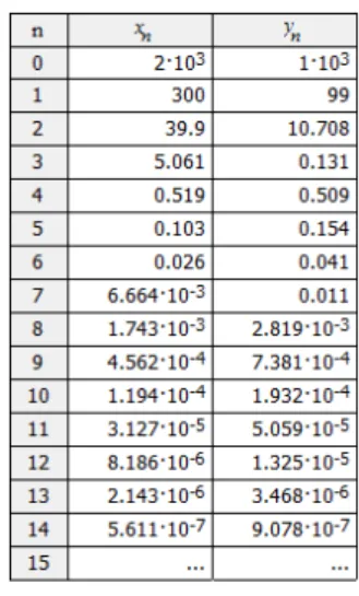
1(a) exhibits that (0; 0) is the global attractor. One can see that the rst and second components of F both converge to 0 quickly as the iteration increases in gure 1(b) and 1(c) (notice that variable n represents the times of iteration).
Figure 1: the dynamic diagram and the iterate diagrams of two components of the example for theorem 2.2
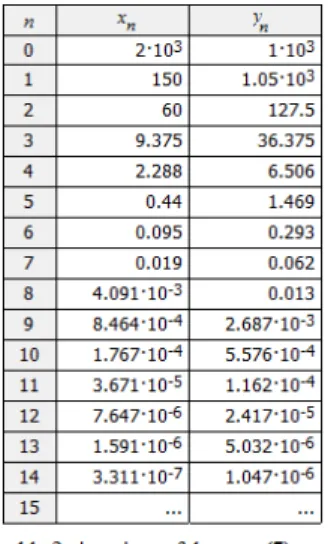
Next, consider the dynamic of another example for theorem 2.3. De ne f (x) = jxj and let a = 2, b = 0:1, p = 10 and q = 0. Then M = 1 and max ab;
1 ap + max abq2 + M a; 1 a b q
ap = 0:55 < 1, which satis es the hypothesis of theorem 2.3. We
also set the initial point (x0; y0) = (2000; 1000). Figure 2(a) exhibits (0; 0) is the global
attractor and gure 2(b),(c) exhibit the situation that two components of F converge.
Figure 2: the dynamic diagram and the iterate diagrams of two components of the example for theorem 2.3
Therefore, the two examples verify the validity and the practicability of theorems 2.2 and 2.3.
9.2
Examples for theorems 2.6, 2.7, 2.8 and 2.9
First, we produce an example for theorem 2.6. Choose a set of special values of a; b; p; q and f as a = 1, b = 0:1, p = 0:01, q = 0 and f (x) = 0:95 sin x. Now we check whether such values and f can satisfy the hypotheses of the theorem. Clearly, 0:95 sin x has countably many simple zeros on R. We choose I = 2 ;
3
2 and V =;. Then qx + f (x) = f (x)
is C1 on 2 ;
3
2 and has two simple zeros 0; in int 2 ; 3
2 = 2 ; 3
2 . The result
p 2 (0; ) means that p approaches to 0 very closely. Since the system (6) is unde ned when p = 0, we just consider the dynamic for p = 0:01. Observe the dynamic in gure 3 for theorem 2.6 with an initial point (x0; y0) = (0:01; 0:02). We see that there is an
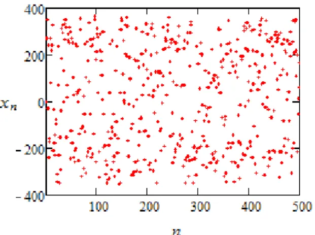
irregular graph in the xplane. We can also see the graphs of iteration of x- and y-components of (6) in gures 4 and 5.
Figure 4: the graph of iteration of x-component of (6) with iterating times from 1 to 500 for theorem 2.6
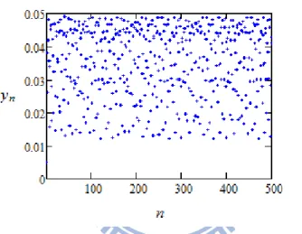
Figure 5: the graph of iteration of y-component of (6) with iterating times from 1 to 500 for theorem 2.6
To observe whether the perturbation of parameter does work, gure 6 shows the bifurcation about p around p = 0:01. We choose the interval of variation of p as [0:001; 1] and also x q = 0. With a di erent value of p, the system begins with a randomly-selected initial point. Afterward, print the second component of the 1000th to 1500th iterations.
Figure 6: the bifurcation diagram of 2nd component of the map (6) about p of the example for theorem 2.6
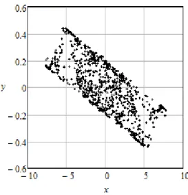
Next, for theorem 2.7, we let a = 6; b = 1; p = 0:01; q = 0 and de ne f (x) = x(1 x). Then f is C1 on [ 0:1; 1:1] and has two simple zeros 0; 1 in int ([ 0:1; 1:1]) = ( 0:1; 1:1). Figure 7 informs us that the system (7) also exhibits a messy diagram with an initial point (0:01; 0:02). We also show the graphs of iteration of two components of (7) in gures 8 and 9.
Figure 8: the graph of iteration of x-component of (7) with iterating times from 1 to 500 for theorem 2.7
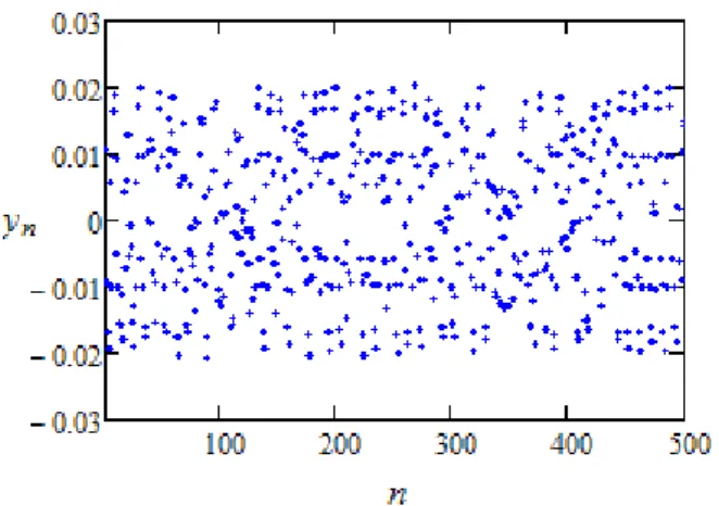
Figure 9: the graph of iteration of y-component of (7) with iterating times from 1 to 500 for theorem 2.7
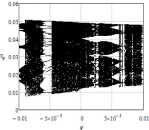
Additionally, we also show the bifurcation diagrams of the second component about p and q individually as follows (see gure 10 for p and gure 11 for q with random initial points). Choose the intervals of variation of p and q as [0:009; 0:012] and [ 0:01; 0:01] respectively.
Figure 10: the bifurcation diagram of 2nd component of the map (7) about p of the example for theorem 2.7 and q = 0 xed
Figure 11: the bifurcation diagram of 2nd component of the map (7) about q of the example for theorem 2.7 and p = 0:01 xed
For theorem 2.8, since a cannot be zero, we consider the case that a = 0:0025, b = 0:001, p = 1, q = 0 and f (x) = 1:1 10 5sin x. It's clear that f is analytic on
[0; ]n (r1; r2) for 0 < r1 < r2 < and 11 sin r1 = 11 sin r2 = . The parametric map
gu(x) = u sin x has period-doubling property (see gure 12 with u from 0 to 35). We have q
b2px + 1
b2pf (x) = 11 sin x 34:56 sin x and 1:1 sin ([0; ]n (r1; r2)) = [0; ]. Since q
b2px + 1
b2pf (x) has a 3-periodic point, whose period is not a power of 2, by theorem A
in [7], we get that htop b2qpx + 1
b2pf (x) > 0. Thus, the hypothesis 2 of theorem 2.8 is
Figure 12: the bifurcation diagram of gu with u from 0 to 35
Next, its dynamic diagram with the initial point (0:001; 0:002) is shown in gure 13. We can see that its shape curls and the points on the graph are not uniformly dense.
The graphs of the two components of this example are shown in gures 14 and 15. It is observable that the situations of iterating of them act not so regularly.
Figure 14: the graph of iteration of x-component of (6) with iterating times from 1 to 500 for theorem 2.8
Figure 15: the graph of iteration of y-component of (6) with iterating times from 1 to 500 for theorem 2.8
For theorem 2.9, consider a = 5, b = 1, p = 0:01, q = 1:11 and f (x) = sin x. Then f is analytic on [0; ]n (r1; r2) for 0 < r1 < r2 < and 1:1 sin r1 = 1:1 sin r2 = . Moreover,
since 1qf (x) = 1:1 sin x, 1qf ([0; ]n (r1; r2)) = [0; ] and htop 1qf > 0. Similarly, we
also show its dynamic diagram and the graphs of iteration of components with the initial point (0:001; 0:002) (see gures 16, 17 and 18).
Figure 16: the dynamic diagram the example for theorem 2.9
Figure 17: the graph of iteration of x-component of (7) with iterating times from 1 to 500 for theorem 2.9
Figure 18: the graph of iteration of y-component of (7) with iterating times from 1 to 500 for theorem 2.9
We set its bifurcation diagram about the parameter p in the interval of variation [0:009; 0:02] in gure 19. The system (7) has the similar dynamic for a = 5, b = 1, q = 1:11 and f (x) = sin x when p is around 0:01.
Figure 19: the bifurcation diagram of 2nd component of the map (7) about p of the example for theorem 2.9
Therefore, theorems 2.8 and 2.9 are applicable.
9.3
Examples for theorems 2.10 and 2.11
We give two examples for theorems 2.10 and 2.11 respectively in this subsection.
For theorem 2.10, consider the case a = 3:91 ; b = 0; p = 3:9; q = 0 and f (x) = x (1 x). Then we see that f is continuous on R and a2qpy +
1 af
1
apy = 3:9y (1 y). It's known
Now we see the dynamic diagram in gure 20 and the graphs of iteration of two components in gures 21 and 22. Choose the initial point (x0; y0) = (0:01; 0:02).
Figure 20: the dynamic diagram the example for theorem 2.10
Figure 21: the graph of iteration of x-component of (6) with iterating times from 1 to 500 for theorem 2.10
Figure 22: the graph of iteration of y-component of (6) with iterating times from 1 to 500 for theorem 2.10
The shape of gure 20 is like a part of a parabola and its distribution is not uniform. So it satis es some characteristics of chaotic graphs. Figure 23 is the bifurcation diagram about b in [ 0:01; 0:01].
Figure 23: the bifurcation diagram of 2nd component of the map (6) about b of the example for theorem 2.10
For theorem 2.11, consider another case a = 1; b = 0; p = 1; q = 0 and f (x) = 1920 sin x. Clearly, f is continuous on R. Since a21pf ( x) = f ( x) = f (x) and
1 af
1
apx = f (x),
we have that f 21;2021 = f 21 ;1920 21;2021 ( f 21 = f 2021 0:445, 21 0:15). The parametric map gu(x) = u sin (x) has also period-doubling property and
htop(f ) > 0 (it has 3-periodic points). Thus, the hypothesis of theorem 2.11 is satis ed.
Next, see the dynamic diagram in gure 24. Moreover, gures 25 and 26 are the graphs of iteration of x- and y-components of (7).
Figure 24: the dynamic diagram the example for theorem 2.11
Figure 25: the graph of iteration of x-component of (7) with iterating times from 1 to 500 for theorem 2.11
Figure 26: the graph of iteration of y-component of (7) with iterating times from 1 to 500 for theorem 2.11
Due to the result pb2+ q2 <
0 for some 0 > 0, we print two bifurcation diagrams
about b and q respectively (see gures 27 and 28). So we can observe the chaotic property.
Figure 27: the bifurcation diagram of 2nd component of the map (7) about b of the example for theorem 2.11 and q = 0
Figure 28: the bifurcation diagram of 2nd component of the map (7) about q of the example for theorem 2.11 and b = 0
References
[1] V S Afraimovich and L A Bunimovich 2007 Dynamical networks: interplay of topol-ogy, interactions and local dynamics Nonlinearity 20 1761{71
[2] V S Afraimovich, L A Bunimovich and S V Moreno 2010 Dynamical networks: con-tinuous time and general discrete time models Regular and Chaotic Dynamics Vol. 15 Nos. 2{3 127{45
[3] V S Afraimovich and S-B Hsu 2003 Lectures on chaotic dynamical systems AMS Studies in Advance Mathematics vol 28 (Providence, RI: American Mathematical Society)
[4] V M Alekseyev 1976 Symbolic dynamics 11th Summer Mathematical School (Kiev: Mathematical Institute of UkAS) (in Russian)
V M Alekseyev 1981 Translations of the AMS (Series 2) vol 116 (Providence, RI: American Mathematical Society) (Engl. Transl.)
[5] R Bowen 1971 Entropy for group endomorphisms and homogeneous spaces Trans. Amer. Math. Soc. 153 401-14
[6] V Coti Zelati and P H Rabinowitz 1991 Homoclinic orbits for a second order Hamil-tonian systems possessing superquadratic potentials J. Amer. Math. Soc. 4 693{727 [7] J Hu and C Tresser 1998 Period doubling, entropy, and renormalization Fundamenta
Mathematicae 155 237-49
[8] J Juang, M-C Li and M Malkin 2008 Chaotic di erence equations in two variables and their multidimensional perturbations Nonlinearity 21 1019{40
[9] M Ma and Z Guo 2006 Homoclinic orbits for second order self-adjoint di erence equations J. Math. Anal. Appl. 323 513{21
[10] T Mitra 2001 A Su cient Condition for Topological Chaos with an Application to a Model of Endogenous Growth Journal of Economic Theory 96 133-52
[11] M-C Li, M-J Lyu and P Zgliczynski 2008 Topological entropy for multidimen-sional perturbations of snap-back repellers and one-dimenmultidimen-sional maps Nonlinearity 21 2555{67
[12] M-C Li and M Malkin 2006 Topological horseshoes for perturbations of singular di erence equations Nonlinearity 19 795{811
[13] K Tanaka 1991 Homoclinic orbits in a rst-order superquadratic Hamiltonian system: Convergence of subharmonic orbits J. Di erential Equations 94 315{39