國 立 交 通 大 學
資訊科學與工程研究所
博士論文
適用於無線感測網路之節能路由與中繼感測器安置演算法
Energy-Aware Routing and Relay Sensors Placing
Algorithms in Wireless Sensor Networks
研 究 生:張志輝
指導教授:簡榮宏 博士
適用於無線感測網路之節能路由與中繼感測器安置演算法
Energy-Aware Routing and Relay Sensors Placing
Algorithms in Wireless Sensor Networks
研 究 生: 張志輝 Student: Jyh-Huei Chang
指導教授: 簡榮宏 博士 Advisor: Dr. Rong-Hong Jan
國立交通大學
資訊科學與工程研究所
博士論文
A Dissertation
Submitted to Institute of Computer Science and Engineering
College of Computer Science
National Chiao Tung University
in partial Fulfillment of the Requirements
for the Degree of
Doctor of Philosophy
in
Computer Science
November 2011
適用於無線感測網路之節能路由與中繼感測器安置演算法
研究生: 張志輝 指導教授: 簡榮宏 博士
國 立 交 通 大 學 資 訊 科 學 與 工 程 研 究 所
摘 要
無線感測網路 (wireless sensor networks, WSNs) 是由許多散佈於各地的感測節點 (sensor nodes) 所組成,主要用以蒐集各種環境資料,例如溼度、壓力、溫度等。
節能路由與中繼感測器安置是無線感測網路重要的研究議題,在本論文中我們提出數種 適用於無線感測網路之節能路由與中繼感測器安置演算法 (relay sensors placing
algorithm),其中包括兩種節能叢集路由演算法 (energy-aware cluster-based routing algorithms), 兩種訊息渡輪路由演算法 (message ferry routing algorithms), 及一種中 繼感測器安置演算法。
在節能路由 (energy-aware routing) 議題中, 叢集路由演算法 (cluster-based routing algorithm), 具有增加擴展性與有效性之優點, 如何以叢集路由演算法來最大化無 線感測網路之生命週期 (lifetime) 亦是一個重要的研究議題。
針對節能路由議題,我們提出兩種適用於無線感測網路的節能叢集路由演算法
(cluster-based routing algorithm), 稱為 ECRA 及 ECR-2T。ECRA 及 ECRA-2T 之效能優 於其他演算法。 這是因為 ECRA 及 ECRA-2T 旋轉叢集頭 (intra-cluster-heads)以平衡每 個感測器的負荷量。 ECRA-2T 具有縮短傳輸距離的優點。
有關訊息渡輪路由 (message ferry routing) 議題, 在特殊環境裡, 例如戰場、疫 區、廣域監視區等, 大多數路由演算法無法將接收到的訊息傳送至目的地。 因此, 如何在 分離的無線感測網路 (partitioned wireless sensor networks) 中收集資料, 是一個重要 的研究議題。
針對訊息渡輪路由議題,我們提出兩種適用於有容量限制(buffer-limited) 的無線感 測網路的路由演算法, 稱為 MFRA1 及MFRA2。MFRA1 及 MFRA2 將原拜訪路徑 (initial visit sequence) 分割成一些次路徑 (sub-sequences), 在一個完整的拜訪順序中 (a complete sequence), 過載感測器 (overflow sensor) 會被 message ferry 拜訪兩次, 因 此能繼續正常運作。 MFRA1 及MFRA2 在資料遺失量 (the amount of data loss) 之效能優 於其他演算法。 因為其他方法忽略了感應器的過載 (overflow) 問題。
在中繼感測器安置 (relay sensors placing) 議題中, 隨機部署的無線感測網路中, 存在通訊缺口(communication gaps), 如何以最少的中繼感測器來保持網路連通, 是一個重 要的研究議題。
針對中繼感測器安置 (relay sensors placing) 議題,我們提出一種適用於無線感測 網路的中繼感測器安置演算法, 稱為 ERSPA。 ERSPA 在平均中繼感測器數量的效能優於 Minimum Spanning Tree 演算法及 Greedy 演算法。 Minimum Spanning Tree 演算法所需 的平均中繼感測器數量約為 ERSPA 的兩倍。 這是因為 ERSPA 將中繼感測器安置在最佳位 置以連通整個感測網路。
Energy-Aware Routing and Relay Sensors
Placing Algorithms in Wireless Sensor Networks
Student: Jyh-Huei Chang Advisor: Dr. Rong-Hong Jan
Institute of Computer Science and Engineering National Chiao Tung University
Abstract
In WSNs, there are spatially distributed sensors which cooperatively monitor environmental conditions, such as humidity, pressure, temperature, motion, or vibration, at different locations. Energy-aware routing and relay placing problems are important research issues in wireless sensor networks. In this dissertation, we design several efficient algorithms in wireless sensor networks, including two kinds of energy-aware cluster-based routing algorithms, two kinds of message ferry routing algorithms, and a relay placing algorithm.
In energy-aware routing problem, cluster-based routing protocols have special advantages that help enhance both scalability and efficiency of the routing protocol. Likewise, finding the best way to arrange clustering so as to maximize the network’s lifetime is now an important research topic in the field of wireless sensor networks. For energy-aware routing problem, we propose an energy-aware cluster-based routing algorithm (ECRA) for wireless sensor networks to maximize the network’s lifetime. The ECRA selects some nodes as cluster-heads to construct Voronoi diagram and rotates the cluster-head to balance the load in each cluster. A two-tier architecture (ECRA-2T) is also proposed to enhance the performance of the ECRA. The simulations show that both the ECRA-2T and ECRA algorithms outperform other routing schemes such as direct communication, static clustering and LEACH. This strong performance stems from the fact that the ECRA and ECRA-2T rotate intra-cluster-heads to balance the load to all nodes in the sensor networks. The ECRA-2T also leverages the benefits of short transmission distances for most cluster-heads in the lower tier.
In message ferry routing problem, some particular environments such as battle-field, disaster recovery and wide area surveillance, most existing routing algorithms will fail to deliver messages to their destinations. Thus, it is an important research issue of how to deliver data in disconnected wireless sensor networks.
For message ferry routing problem, we propose two efficient message ferry rout-ing algorithms in partitioned and buffer-limited wireless sensor networks, denoted as MFRA1 and MFRA2. MFRA1 and MFRA2 fix the overflow by partitioning the initial visit sequence into some sub-sequences such that the ferry visits the over-flow node twice in the resulting sequence. The above process will continue until a feasible solution is found. Simulation results show that both MFRA1 and MFRA2 are better than other schemes in terms of the amount of data loss, because the other schemes neglect the case of sensor overflow.
In relay placing problem, randomly deployed sensor networks often make initial communication gaps inside the deployed area, even in an extremely high-density network. How to add relay sensors such that the underlying graph is connected and the number of relay sensors added is minimized is an important problem in wireless sensor networks.
For relay placing problem, we propose an efficient relay sensors placing algo-rithm (ERSPA) for disconnected wireless sensor networks. Compared with the minimum spanning tree algorithm and the greedy algorithm, ERSPA achieves bet-ter performance in bet-terms of the number of relay sensors added. Simulation results show that the average number of relay sensors added by the minimal spanning tree algorithm is approximately two times that of the ERSPA algorithm. This is because ERSPA places the relay sensors in optimal places to connect the maxi-mum number of initial connected sub-graphs such that the average number of relay sensors can be minimized.
Acknowledgements
Special thanks goes to my advisor Professor Rong-Hong Jan for his guidance in my dissertation work and the instructions on writing articles. Thanks also to all members of Computer Network Lab for their assistance and kindly help in both the research and the daily life during these years. Finally, I will dedicate this dissertation to my families for their love and support.
Contents
Abstract(in Chinese) i
Abstract(in English) iii
Contents vi
List of Tables viii
List of Figures ix
1 Introduction 1
2 Energy-aware routing problem for general WSNs 6
2.1 Related works of energy-aware routing problem . . . 6
2.2 Problem formulation and network model . . . 9
2.3 Solution methods for energy-aware routing problem . . . 10
2.3.1 Three phases of ECRA . . . 10
2.3.2 Enhancement of ECRA . . . 15
2.4 Simulation results . . . 17
2.4.1 Performance metrics and environment setup . . . 17
3 Message ferry routing problem for partitioned and buffer-limited
WSNs 26
3.1 Related works for message ferry routing problem . . . 26
3.2 Problem formulation and network model . . . 28
3.2.1 Network model . . . 28
3.2.2 Problem formulation . . . 29
3.3 Solution methods for message ferry routing problem . . . 33
3.3.1 MFRA1 . . . 33
3.3.2 MFRA2 . . . 37
3.4 Simulation results . . . 40
3.4.1 Performance metrics and environment setup . . . 40
3.4.2 Numerical results . . . 41
4 Relay placement problem for disconnected WSNs 47 4.1 Related works of relay placement problem . . . 47
4.2 Problem formulation and network model . . . 49
4.3 Solution methods for relay placement problem . . . 50
4.4 Simulation results . . . 60
4.4.1 Performance metrics and environment setup . . . 60
4.4.2 Numerical results . . . 60
List of Tables
List of Figures
1.1 Example of message ferry scheme. . . 4
2.1 Wireless sensor network organized in clusters. . . 8
2.2 The examples of CVTs for n = 2, 3, 4, 5. . . 12
2.3 Voronoi diagram of the 100-node random sensor network with
cen-troidal points. . . 13
2.4 Voronoi diagram of the 100-node random sensor network without
centroidal points. . . 13
2.5 The operation of two-tier architecture in enhanced ECRA, where T
isthe current round and T + d is the next round, and so on. . . 16
2.6 The normalized total energy dissipation related to different
percent-age of cluster-heads in ECRA. . . 19
2.7 The lifetime of first node died (FND) under different methods. The
initial energy of each sensor is 1 Joule. . . 22
2.8 The lifetime of first node died (FND) using different amounts of
initial energy for the sensors. . . 23
2.9 The lifetime of last node died (LND) under different methods. The
2.10 The lifetime of last node died (LND) using different amounts of
initial energy for the sensors. . . 24
2.11 Total energy dissipation (TED) using direct communication, LEACH, ECRA, and ECRA-2T. The messages are 2000 bits. . . 24
2.12 Number of alive nodes under different routing schemes. The initial energy of each sensor is 1 Joule. . . 25
2.13 (a)Energy×Delay cost for different routing schemes in a 50 m x 50 m network. (b)Energy×Delay cost for different routing schemes in a 100 m x 100 m network. . . 25
3.1 (a) Ten sensors in the sensing field. (b) A least cost visit sequence with one critical node (Node n1). (c) A feasible complete sequence n1, n2, n3, n4, n5, n1, n6, n7, n8, n9, n10, n1. . . 31
3.2 An illustrated example of MFRA1. . . 35
3.3 The solution space of MFRA1 for the example. . . 38
3.4 An illustrated example of MFRA2. . . 39
3.5 The solution space of MFRA2. . . 40
3.6 The travel time vs. the number of critical nodes for MFRA1 (MFRA2) with 5 and 10 sensors. . . 43
3.7 The number of checked sequences of MFRA1 and MFRA2 algorithms. 44 3.8 The number of feasible solutions of MFRA1 and MFRA2 algorithms. 44 3.9 The amount of data loss for different methods. . . 45 3.10 The amount of data loss for different buffer sizes with 3 critical nodes. 45 3.11 The amount of data loss for different buffer sizes with 2 critical nodes. 46
4.1 An example of constructing Delaunay using 30 terminal nodes. The thin solid lines represent the edges of the Delaunay triangulation that are not connected. The initial disconnected terminal nodes
are indicated by the ′•′-sign. The initial connected sub-graphs are
indicated by the thick solid lines. . . 51
4.2 An example of lemma 1. . . 52
4.3 (a) An example of four nodes covered by a minimum circle of radius
R. (b) An example of five nodes covered by a minimum circle of
radius R. . . 52
4.4 An example of adding relay sensors after step 2 of phase 2 for the
ERSPA algorithm. Placing one relay node to connect three nodes is
indicated by the circle centered at R1, R2 and R3. The relay sensors
are indicated by the ′∗′-sign. . . . 56
4.5 The connected sub-graphs after steps 3 and 4 of phase 2 in the
ERSPA algorithm. . . 57
4.6 The final connected communication graph. The transmission range
is 10 percent of the side of the square sensing field. . . 59
4.7 (a) The average number of relay nodes for connectivity with 50
ter-minal nodes (b) The average number of relay nodes for connectivity with 90 terminal nodes. The transmission range is 10 percent of the
4.8 (a) The average number of relay nodes for connectivity with 30 terminal nodes. The transmission range is 10 percent of the side of the square sensing field. (b) The average number of relay nodes for connectivity with 30 terminal nodes. The transmission range is 12
percent of the side of the square sensing field. . . 62
4.9 The average number of relay nodes for connectivity under different
terminal nodes. The transmission range is 10 percent of the side of
the square sensing field. . . 63
4.10 The average number of relay nodes for connectivity under different terminal nodes. The transmission range is 12 percent of the side of
Chapter 1
Introduction
In recent years, the Micro-Electro-Mechanical Systems (MEMS) technologies have been booming. These MEMS technologies combined with advances in the wireless communication, make it possible to deploy low-cost, and low-power sensor networks. A wireless sensor network (WSN) consists of a large number of sensor nodes working together to monitor a region to obtain data about the environment [1]. The applications for WSN include environment exploration, military target tracking and surveillance, natural disaster relief, biomedical health monitoring, and seismic sensing. There are two types of WSN: structured and unstructured. In a structured WSN, the sensor nodes are deployed in a pre-planned manner. The advantage of a structured network is that fewer nodes can be deployed with lower network maintenance and management cost. An unstructured WSN is one that contains a dense collection of sensor nodes. In an unstructured WSN, network maintenance such as managing connectivity and detecting failures is difficult [2].
Many studies focus on the following potential applications for WSN:
1) Environment exploration: In environmental monitoring, a WSN can moni-tor air soil and water[3].
2) Military target tracking and surveillance: In military target tracking and surveillance, a WSN can assist in intrusion detection and identification such as spatially-correlated and coordinated troop and tank movements [5,6].
3) Natural disaster relief: In natural disasters, sensor nodes can detect the environment to forecast disasters before they occur [7].
4) Biomedical health monitoring: In biomedical applications, surgical im-plants of sensors can help monitor a patient’s health [8,9].
5) Seismic sensing: For seismic sensing, sensor nodes can detect the development of eruptions and earthquakes [10].
In spite of these diverse applications, most sensor networks encounter the fol-lowing operational challenges:
1) Ad hoc deployment: The sensor networks should be able to cope with the resultant distribution and connection between the nodes.
2) Unattended operation: In most cases, once deployed, sensor networks have no human intervention. Hence the sensor nodes are responsible for reconfiguration in case of any changes.
3) Untethered: The sensor nodes are not connected to any energy source. There is only a finite source of energy, which must be optimally used for processing and communication. The communication dominates processing in energy consumption. Thus, in order to make optimal use of energy, communication should be minimized as much as possible.
4) Dynamic changes: Dynamic environmental conditions require the sensor net-works to be adaptive in nature to change connectivity and node failure [4].
A number of studies propose solutions to one or more of the above challenges for WSNs [1, 2]. In this dissertation, we focus on the following issues which are
important for WSNs:
1) Energy consumption: Energy consumption is the most important factor to determine the lifetime of a sensor network because sensor nodes only have a small and finite source of energy. Many solutions, both hardware and software related, have been proposed to optimize energy usage.
2) Routing: Communication costs play a great role in deciding the routing tech-nique. Conventional routing protocols have several limitations when being used in sensor networks due to the energy constrained nature of these networks. The rout-ing protocols designed for sensor networks should be able to overcome the energy constraint and look at newer ways of conserving energy to increase the lifetime of the network.
3) Localization: In most of the cases, sensor nodes are deployed in an ad hoc manner. It is up to the nodes to identify themselves in some spatial co-ordinate system. This problem is referred to as localization. Many studies proposed the solutions to ensure optimum placement of nodes. Mostly, problems arise due to the unpredictable nature of environmental conditions. Nodes thus will also need to be able to adapt to environmental changes.
Thus, in this dissertation, we consider three important problems which are energy-aware routing problem, message ferry routing problem and relay placement problem.
In energy-aware routing problem, the power for sensor nodes comes from their batteries. Thus, finding the best use for the limited battery power is a crucial research issue in wireless sensor networks. Cluster-based routing protocols have special advantages that help enhance both scalability and efficiency of the routing protocol. Likewise, finding the best way to arrange clustering so as to maximize
Message Ferry Message Ferry Route
Rendezvous Node
Disconnected sub-network
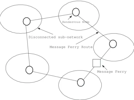
Figure 1.1: Example of message ferry scheme.
the network’s lifetime is now an important research topic in the field of wireless sensor networks.
In message ferry routing problem, a partitioned wireless sensor networks, most existing routing algorithms will fail to deliver messages to their destinations. The Message Ferry scheme is an approach for message delivery in the disconnected wireless sensor network. As shown in Fig. 1.1, there is a wireless sensor network with several separated sub-networks. Each sub-network has a rendezvous node to connect and buffer the data. A special node, called Message Ferry, visits these rendezvous nodes to collect the buffered data of the sensing field based on a pre-defined route. The message ferry route problem is to find a route for message ferry to visit rendezvous nodes and collect data.
The previous schemes focus on the routing problems under the assumption that the buffer size of each sensor node is unlimited. These schemes do not deal with
the condition that the sensor may overflow and thus the sensing data will lose.In real applications, there are different kinds of sensors such as surveillance sensors and data sensors. The surveillance sensor has high sampling rate to capture video messages. The data sensor has low sampling rate to collect temperature or noise data. In such a sensing environment, each sensor has a limited buffer size and thus the surveillance sensor may overflow before the message ferry visits all sensor nodes. It is a serious problem that a sensor loses critical messages due to overload. Therefore, how to avoid overflow should be an important research issue in the message ferry routing problem.
In relay placement problem, randomly deployed sensor networks often make initial communication gaps inside the deployed area, even in an extremely high-density network. How to add relay sensors such that the underlying graph is connected and the number of relay sensors added is minimized is an important problem in wireless sensor networks.
Our solution methods can connect the heterogeneous wireless sensor networks and gather data to base station.
The rest of this dissertation is organized as follows. In Chapter 2, we introduce the energy-aware routing problem and our solution methods for general WSNs. Next, we illustrate the message ferry routing problem and our solution methods for partitioned and buffer-limited WSNs in Chapter 3. The relay placement problem and our solution methods for disconnected WSNs will be described in Chapter 4. Finally, a conclusion is given in Chapter 5.
Chapter 2
Energy-aware routing problem for
general WSNs
In this chapter, we first describe related works of energy-aware routing problem. Then, we illustrate problem formulation and our solution methods. Finally, we present simulation results of our scheme.
2.1
Related works of energy-aware routing
prob-lem
Many studies have focused on saving energy in different ways such as reducing the power spent on the modulation circuits [11], or managing the power usage on the MAC layer of sensor nodes [12-13]. However, these schemes focused of the indi-vidual device, and that approach is too narrow when working with wireless sensor networks. Since sensor nodes have limited transmitting ranges, only a few nodes can communicate directly with the sink node. In most cases, the sensor nodes gather sensing data which must then be forwarded by the other node to the sink node. However, these cumbersome relaying operations consume too much energy, thus causing the relay nodes to rapidly expend much of their power. Therefore,
developing a load-balanced routing algorithm to maximize the network’s lifetime has become an important research topic.
A large number of routing protocols [14-20] for wireless sensor networks have been proposed, but most are flawed in one way or another. In the fixed path schemes [14-15], sensor nodes arrayed in a fixed path will consume much energy and get exhausted rapidly because they continually provide relaying service. The flooding scheme consumes too much energy for relaying duplicate packets. Source routing schemes [16-17] solved some of the drawbacks of the flooding approach; however, they can not operate well when the number of hops between the source and sink is large. Energy-aware, multi-path routing schemes [18-20] have the ad-vantage of sharing the energy among all the sensors in the wireless networks. Nev-ertheless, the chief disadvantage of multi-path routing schemes [18-19] is that the sensor nodes only keep a local view of energy usage and the nodes in the network can not have an even traffic dispatch.
In addition, many studies have focused on cluster-based energy-efficient rout-ing protocol for wireless sensor networks [21-35]. Power-Efficient Gatherrout-ing in Sensor Information Systems (PEGASIS) [31] prolongs the network lifetime with a chain topology. But the delay is significant although the energy is saved. Hybrid Energy-Efficient Distributed Clustering (HEED) [32] considers a hybrid of residual energy and communication cost when selecting cluster-head. A sensor has high-est residual energy can become a cluster-head. However, if the residual energy of the sensors in a cluster is nearly the same, it takes many iterations and expends much energy to elect cluster-head. The Low Energy Adaptive Clustering Hierar-chy (LEACH) [33-34] randomly selects some nodes as cluster-heads and rotates the cluster-head to distribute the load to all sensors in the wireless sensor networks. Its
Sink CH N Cluster−head (CH) Sensor Node (N) N N
Figure 2.1: Wireless sensor network organized in clusters.
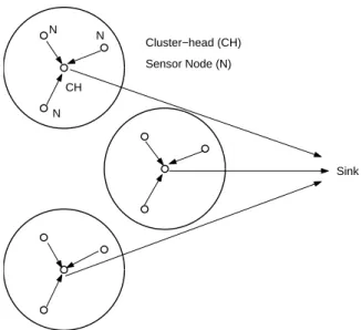
performance is better than that of the direct communication and static clustering routing protocols. Figure 2.1 shows an example of the cluster-based routing scheme for wireless sensor networks. In Figure 2.1, each cluster has one cluster-head. The non-cluster-head nodes transmit their sensing data to cluster-heads which then forward the aggregated data to the sink node. The use of clusters leverages the benefits of short transmission distances for most nodes. The cluster-head acts as a fusion point to aggregate the sensing data so that the amount of data that is actually transmitted to the sink node is reduced [23-24]. Thus, network clustering can increase system lifetime and energy efficiency. Cluster-based routing protocols have special advantages: they can enhance the scalability and efficiency of the routing protocol to reduce the routing complexity [35], reduce the complexity of location management [36], and improve the power control procedure [37]. However, LEACH may also have several problems: First, if the coverage of the cluster-heads
is too small, then some cluster-heads may not have any members in their clusters. Second, LEACH has a long transmission range between the cluster-heads and the sink node. Third, the LEACH requires global heads rotation. This cluster-head selection greatly increases processing and communication overcluster-head, thereby consuming more energy.
2.2
Problem formulation and network model
The network model and assumptions of our research are described as follows: 1) All sensors are location aware. That is, they can convey their location informa-tion to the base stainforma-tion in the initializainforma-tion phase (phase 0). 2) The base stainforma-tion has a power supply so we assume it has infinite energy. Therefore, the energy required for the base station to inform each cluster-head can be ignored. 3) Base stations can compute the residual energy of all sensors in each round according to their location and the amount of transmission data.
The energy model of our study is the same as in [33]. In this energy model,
the electronic energy Eelec = 50 nJ/bit in needed to operate the transmitter or
receiver circuit. The transmitter amplifier is ǫamp = 100 pJ/bit/m2. Equations
(2.1) and (2.2) are used to calculate the transmission energy, denoted as ET x(k, d),
required for a k bits message over a distance of d,
ET x(k, d) = ET x elec(k) + ET x amp(k, d) (2.1)
= Eelec× k + ǫamp× k × d2. (2.2)
To receive this message, the energy required is:
where ET x elecis the energy dissipation of transmitter electronics and ERx elec is
the energy dissipation of receiver electronics. ET x ampis the energy of the
transmit-ter amplifier. Assume that ET x elec = ERx elec = Eelec. From equation (2.3), one
can see that receiving data is also a high overhead procedure. Thus, the number of transmission and receiving operations must be cut to reduce the energy dissi-pation. We also assume that the radio channel is symmetric such that the energy required to transmit a message from node i to node j is the same as the energy required to transmit a message from node j to node i for a given signal-to-noise ratio.
2.3
Solution methods for energy-aware routing
problem
2.3.1
Three phases of ECRA
Our ECRA algorithm includes three phases: clustering, data transmission and intra-cluster-head rotation. The details of the algorithm are given as follows.
Phase 1: Clustering
First, we define of the Voronoi diagram and Centroidal Voronoi Tessellation
(CVT) [38-40]. Consider an open set Ω ⊆ ℜ2 and a set of points {z
i}ni=1 belonging
to ¯Ω where ¯Ω is the closed set of Ω. Let |.| denote the Euclidean norm in ℜ2. The
Voronoi region Vi corresponding to the points zi is defined by
Vi = {x ∈ Ω| |x − zi| < |x − zj| for j = 1, ..., n, j 6= i} (2.4)
where Vi ∩ Vj = ∅ for i 6= j and ∪ni=1V¯i = ¯Ω. The set of {Vi}ni=1 is a Voronoi
The points {zi}ni=1 are called generators.
CVT is a Voronoi tessellation whose generating points are the centroids of mass for their corresponding Voronoi regions. Formally, CVT can be defined as follows.
Given a region Vi ⊆ ℜ2and a density function ρ(x), defined in Vi, the mass centroid
z∗ i of Vi is defined by z∗ i = R Vixρ(x)dx R Vi ρ(x)dx for i = 1, ..., n. (2.5)
Given n points {zi}ni=1, if the points zi=z∗i for i = 1, ..., n, then we call the
Voronoi tessellation defined by equation (2.4) as a CVT. That is, the points zi that
serve as the generators for Voronoi regions Vi are themselves the mass centroids of
those regions. Figure 2.2 shows the CVTs with ρ(x) = c for n = 2, 3, 4, 5.
We apply the following two steps to partition the sensor nodes into n clusters. Step 1: Given sensing field Ω, a positive integer n, and a density function ρ(x) = c,
construct a centroidal Voronoi tessellation such that Vi is the Voronoi region
for z∗
i and zi∗ is the mass centroid of Vi for each i. That is, the sensing field
is partitioned into n Voronoi regions.
Step 2: Let wi, i = 1, . . . , m, denote the sensor nodes in sensing field Ω.
(a) For each node wi, if wi ∈ Vj, then we assign node wi to cluster Cj.
(b) For each Cj, j = 1, . . . , n, find a sensor node w∗j that is closest to z∗j,
the mass centroid of Vj. Then, we choose sensor node w∗j as the initial
cluster head of cluster Cj.
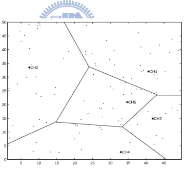
Figure 2.3 shows that these cluster-heads are located nearest their corre-sponding centroidal points. The advantage of the above clustering method is that
0 10 20 30 40 50 0 10 20 30 40 50 0 10 20 30 40 50 0 10 20 30 40 50 0 10 20 30 40 50 0 10 20 30 40 50 0 10 20 30 40 50 0 10 20 30 40 50
Figure 2.2: The examples of CVTs for n = 2, 3, 4, 5.
each cluster head has a nearly equal number of members; this is because the sensor nodes are uniformly distributed. In contrast with Figure 2.3, Figure 2.4 shows the Voronoi diagram in which the generating points were selected randomly. Note that the clusters have diverse number of members.
In the ECRA scheme, we assume that the sensor nodes are location-aware. That is, the base station knows every sensor node’s location. The base station constructs CVT for the sensing field. Each cluster has only one cluster-head. The base station tells each cluster-head which nodes are its member. The cluster-head broadcasts an advertisement to their members. By listening to the advertisement, each node knows which cluster it belongs to. Then, the sensor node sends an ac-knowledgement to its cluster-head and confirms that it will be a member of the cluster. During this time, all cluster-heads must remain in active.
5 10 15 20 25 30 35 40 45 0 5 10 15 20 25 30 35 40 45 50 CH1 CH2 CH3 CH4 CH5 X−coordinate Y−coordinate
Figure 2.3: Voronoi diagram of the 100-node random sensor network with cen-troidal points. 5 10 15 20 25 30 35 40 45 0 5 10 15 20 25 30 35 40 45 50 CH1 CH2 CH3 CH4 CH5
Figure 2.4: Voronoi diagram of the 100-node random sensor network without cen-troidal points.
Phase 2: Data transmission
When the clusters are created, data transmission can begin. The nodes use single hops to communicate with their cluster-heads, and the cluster-heads com-municate with the base station. Each node has M bits messages to transmit. The non-cluster-head node can turned-off until its allocated transmission time in order to minimize the energy usage. When all data from the nodes have been received, the cluster-head aggregates the total data into a single message to reduce the amount of information transmitted to the base station.
Phase 3: Intra-cluster-head rotation
When a round is ended, next rotate the cluster-head within the same cluster
based on a parameter called Oij which is a function of communication cost Edij
and residual energy Enew
ij . The distance dij, i = 1, . . . , n, j = 1, . . . , |Ci|, represents
the distance from node j in cluster Ci to the base station and is given as
dij =
q
(xij − x∗)2+ (yij − y∗)2 (2.6)
where (xij, yij) is the position of node j in cluster Ci and (x∗, y∗) is the position of
the base station. The residual energy Enew
ij is defined as Enew ij = Eijold− E expend ij (2.7) where Eold
ij is the residual energy of node j in cluster Ci at the beginning of the
current round. Eijexpend is the energy expended by the node in the current round.
Edij is the energy expended by the cluster-head to transmit data to base station.
Oij =
Enew
ij
Edij
, i = 1, . . . , n, j = 1, . . . , |Ci| (2.8)
For each cluster Ci, we find
O(i) = max{Oij|j = 1, . . . , |Ci|}.
Node j in cluster Ci with the value of O(i) will become a cluster-head of cluster
Ci at the next round. That is, when all data are received in the current round,
the base station first calculates the value of Oij for each node j in cluster Ci, then
finds O(i) for each C
i, and finally informs the node with value O(i) to become the
new cluster-head at the next round. Note that the base station has the location of each node and it also knows that each sensor node has sent M bit messages, and
thus the base station can calculate the value of Oij.
When the current round is ended, the role of the cluster-head will rotate to
the node with value O(i) that is designated by the base station. Then, the new
cluster-head begins to advertise using the method given in phase 1.
2.3.2
Enhancement of ECRA
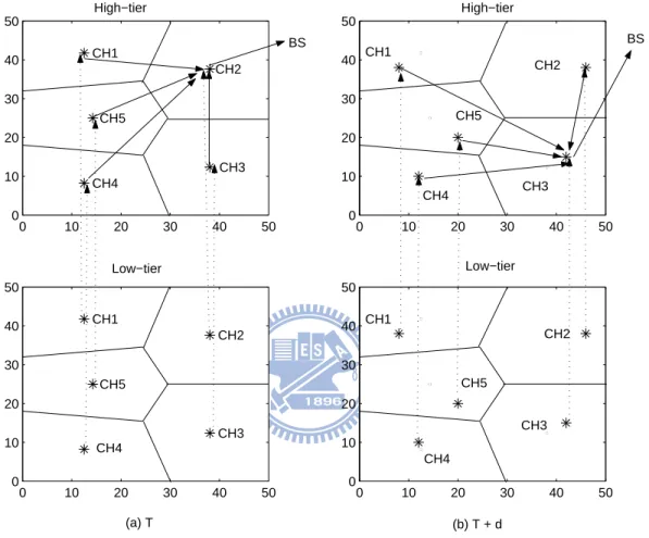
The ECRA can be enhanced by adding an extra tier, called a high tier, on top of the original architecture (see Figure 2.5). The high tier has only one cluster. All cluster-heads in the low tier are also the members in the high tier. This architecture is called a two-tier ECRA (denoted as ECRA-2T). The nodes in the high tier forward their aggregated data to the node with the maximal remaining energy, called the main cluster-head. The main cluster-head transmits the aggregated data to the sink. When a round is over, rotate the cluster-head of the low-tier in
0 10 20 30 40 50 0 10 20 30 40 50 CH1 CH2 CH3 CH4 CH5 0 10 20 30 40 50 0 10 20 30 40 50 CH1 CH2 CH3 CH4 CH5 0 10 20 30 40 50 0 10 20 30 40 50 CH1 CH2 CH3 CH4 CH5 0 10 20 30 40 50 0 10 20 30 40 50 CH1 CH2 CH3 CH4 CH5 BS BS (a) T (b) T + d High−tier High−tier Low−tier Low−tier
Figure 2.5: The operation of two-tier architecture in enhanced ECRA, where T isthe current round and T + d is the next round, and so on.
the high-tier in the next round consist of these cluster-heads. Figure 2.5 illustrates
the high-tier operation in ECRA-2T. In the current round T , CH2 is the main
cluster-head. In next round T + d, CH3 has a maximal remaining energy that is
selected as the main cluster-head, and so on.
2.4
Simulation results
2.4.1
Performance metrics and environment setup
This section presents the performance analysis of the ECRA algorithm. The performance metrics are given as follows.
1) The lifetime for the first node to die (FND): FND is defined as the time required for the first node to run out of energy. The non-cluster-head nodes transmitted their sensing data to the cluster-head. The cluster-heads forwarded their aggre-gated data to the sink periodically. We use the number of rounds to represent the network lifetime of FND. A round is defined as all nodes in the wireless network that finish returning their gathered data to the sink. The time interval between two rounds is assumed to be large enough for the last node to return its sensing data.
2) The lifetime for the last node to die (LND): LND is defined as the time required for the last node to run out of energy, at which time the network crashed. We also use the number of rounds to represent the network lifetime of LND.
3) The total energy dissipation (TED): This value is defined as the energy dissi-pation for all nodes that finish returning their gathered data.
4) The cost of energy×delay: This value is the cost for each round of data gath-ering from sensor node to sink node. The energy cost can be calculated from the
energy model described in Section 2. The delay cost can be calculated as units of time. On a link with 2Mbps, a message of 2000 bits can be transmitted in 1ms. Therefore each unit of delay will be about 1 ms for a sensor node with a single channel. We assume that the delay cost is 1 unit for each message of 2000 bits transmitted.
We evaluate the performance of our study implemented with C++ and MAT LAB.
Four different sizes of deploying regions were simulated: 50 × 50 m2, 100 × 100 m2,
150×150 m2 and 200×200 m2. In each region, 100 nodes were deployed by uniform
distribution. Assume that the energy model is the same as in [33]. The electronics
energy is Eelec = 50 nJ/bit. ǫamp = 100 pJ/bit/m2. The energy of data
aggrega-tion is 5 nJ/bit/message. The cluster-heads use a 1-bit message to inform their members in each round. Then, the members send their data to their cluster-heads. The negotiation energy consumption is included in each round. The sink node was located at the position ((x, y) = (25, −100)). Each sensor has 2000 bits of data sent to the base station during each round.
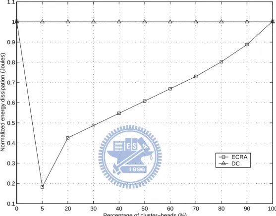
First, we determined the number of cluster header n. Note that if n is small, then the average length from sensor node to its cluster is large. This means that the energy costs between sensor node and cluster head is large. However, if n is large, then the total energy costs between cluster header and the base station is large. By simulation, Figure 2.6 shows the normalized total energy dissipation related to different percentages of cluster-heads in ECRA. From Figure 2.6, we learn that the normalized total energy dissipation is minimized at the 5 % of the total number of sensor nodes for ECRA. Thus, we chose n = 5 from 100 sensor nodes as cluster headers.
0 5 20 30 40 50 60 70 80 90 100 0.1 0.2 0.3 0.4 0.5 0.6 0.7 0.8 0.9 1 1.1 Percentage of cluster−heads (%)
Normalized energy dissipation (Joules)
ECRA DC
Figure 2.6: The normalized total energy dissipation related to different percentage of cluster-heads in ECRA.
2.4.2
Numerical results
Comparisons of the four performance metrics were made for six schemes: the direct communication (DC), static clustering (SC), LEACH, PEGASIS [21], HEED [32], ECRA and ECRA-2T. The results are given as follows.
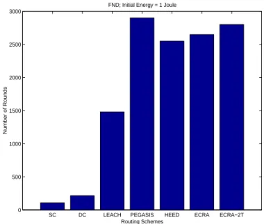
1) The lifetime of FND under different initial energy levels
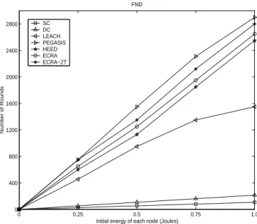
Figure 2.7 shows that of the lifetime of ECRA-2T in FND is better than LEACH, HEED, direct communication, and static clustering if the initial energy of each sensor is 1 J. Figure 2.8 shows the lifetime of FND under different methods with different initial energy of each node. Overall, the life-time of FND increases when the initial energy of each sensor is greater. Both ECRA and ECRA-2T have better performance than other schemes. The life-time of FND in ECRA-2T is approximately twice that of LEACH, but over eight times than that of direct communication and static clustering. That is, ECRA-2T gives better performance than DC, SC, HEED and LEACH in the lifetime of FND.
2) The lifetime of LND under different initial energy levels
Figure 2.9 shows that the lifetime of ECRA-2T in LND is better than that of LEACH, HEED, PEGASIS, direct communication and static cluster-ing if the initial energy of each sensor is 1 J. Figure 2.10 shows the lifetime of LND under different methods with different initial energy of each node. Overall, the lifetime of LND increases when the initial energy of each sen-sor is greater. Both ECRA and ECRA-2T have better performance than other schemes. The lifetime of LND in ECRA-2T is approximately 2.5 times
longer than LEACH but over nine times greater than direct communication and static clustering. The results show that ECRA-2T gives better perfor-mance than DC, SC, PEGASIS, HEED and LEACH in the lifetime of LND. From Figures 2.7 and 2.9, note that if a scheme shares the load evenly with all sensor nodes in the network, it can achieve a longer lifetime.
3) Total energy dissipation under different network diameters
Figure 2.11 shows that ECRA-2T uses much less energy compared to di-rect communication. In other words, using clusters lets one leverage the benefits of short transmission distances for most nodes and distributes the energy among the sensor nodes in the network, thus reducing total energy dissipation.
Figure 2.12 shows the number of alive nodes under different routing schemes. This number decreases when the number of rounds is greater. From Figure 2.12, we note that the performance of ECRA-2T is better than that of LEACH. According to the above analysis, our ECRA-2T algorithm has better performance than do other schemes regarding system lifetime and energy dissipation. These simulation results also show that ECRA-2T has the advantages of balanced loads and saved energy.
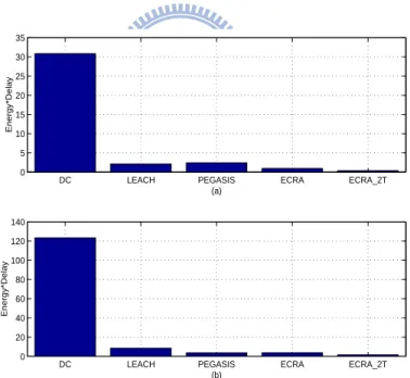
4) The cost of energy×delay: Figure 2.13-(a) shows that ECRA-2T is better than LEACH, PEGASIS, and direct communication for a 50 m × 50 m network in terms of energy×delay. Figure 2.13-(b) shows that ECRA-2T is also better than LEACH and direct communication for a 100 m × 100 m
SC DC LEACH PEGASIS HEED ECRA ECRA−2T 0 500 1000 1500 2000 2500 3000
FND; Initial Energy = 1 Joule
Routing Schemes
Number of Rounds
Figure 2.7: The lifetime of first node died (FND) under different methods. The initial energy of each sensor is 1 Joule.
network in terms of energy×delay. This is because the two-tier architecture leverages the benefits of short transmission distances for most cluster-heads in the low-tier.
0 0.25 0.5 0.75 1.0 0 400 800 1200 1600 2000 2400 2800 FND Number of Rounds
Initial energy of each node (Joules) SC DC LEACH PEGASIS HEED ECRA ECRA−2T
Figure 2.8: The lifetime of first node died (FND) using different amounts of initial energy for the sensors.
SC DC LEACH PEGASIS HEED ECRA ECRA−2T
0 500 1000 1500 2000 2500 3000 3500 4000 4500 5000
LND; Initial Energy = 1 Joule
Routing Schemes
Number of Rounds
Figure 2.9: The lifetime of last node died (LND) under different methods. The initial energy of each sensor is 1 Joule.
0 0.25 0.5 0.75 1.0 0 400 800 1200 1600 2000 2400 2800 3200 3600 4000 4400 4800 LND Number of Rounds
Initial energy of each node (Joules) SC DC LEACH PEGASIS HEED ECRA ECRA−2T
Figure 2.10: The lifetime of last node died (LND) using different amounts of initial energy for the sensors.
0 50x50 100x100 150x150 200x200 0 0.1 0.2 0.3 0.4 0.5 0.6 0.7 0.8 0.9 1 TED Joules Network Size DC LEACH HEED PEGASIS ECRA ECRA−2T
Figure 2.11: Total energy dissipation (TED) using direct communication, LEACH, ECRA, and ECRA-2T. The messages are 2000 bits.
0 20 40 60 80 100 0 400 800 1200 1600 2000 2400 2800 3200 3600 4000 4400 4800
Number of alive nodes
Rounds ECRA−2T ECRA PEGASIS LEACH DC SC
Figure 2.12: Number of alive nodes under different routing schemes. The initial energy of each sensor is 1 Joule.
DC LEACH PEGASIS ECRA ECRA_2T
0 5 10 15 20 25 30 35 (a) Energy*Delay
DC LEACH PEGASIS ECRA ECRA_2T
0 20 40 60 80 100 120 140 (b) Energy*Delay
Figure 2.13: (a)Energy×Delay cost for different routing schemes in a 50 m x 50 m network. (b)Energy×Delay cost for different routing schemes in a 100 m x 100 m network.
Chapter 3
Message ferry routing problem
for partitioned and buffer-limited
WSNs
In this chapter, we first describe related works of message ferry routing problem. Then, we illustrate problem formulation and our solution methods. Finally, we present simulation results of our scheme.
3.1
Related works for message ferry routing
prob-lem
Several schemes have been proposed to solve the message ferry route problem in partitioned wireless ad hoc networks [41-45]. In [41], the authors propose a message ferry scheme to solve the data delivery problem in high-partitioned wireless ad hoc networks. In [42], the authors introduce a non-randomness in the movement of nodes to improve data delivery performance and reduce the energy consumption in sensor nodes. Epidemic routing [44] is also a well-known routing method for partitioned wireless ad hoc networks. In this scheme nodes forward messages to other nodes they meet. However, this scheme transmits many redundant messages.
Compared to Epidemic routing, message ferry scheme is very efficiency in data delivery and energy consumption. However, the synchronization between nodes and ferry is a problem in the message ferry scheme. An optimized way-points (OPWP) algorithm [43] was proposed. It generates a ferry route to achieve good performance without any online collaboration between nodes and the ferry. OPWP outperforms other naive ferry routing schemes.
Many studies deal with efficient routing for intermittently connected mobile ad hoc networks [46-53]. In [46-47], the authors proposed a routing scheme with two types of ferries and gateways. This scheme improves delivery rate and delay without online collaboration between ferry and mobile nodes. However, the local message ferry, global message ferry and gateway nodes of this scheme need more resources to buffer the messages. In [48], the authors proposed single-copy routing schemes that use only one copy per message, and hence significantly reduce the resource requirements of flooding-based algorithms. In [49], the authors proposed a routing scheme that sprays a few message copies into the network, and then routes each copy independently toward the destination. This scheme can reduce the delay in flooding-based scheme.
Some studies deal with the data scheduling problem for message ferry [54-55]. In [54], the authors present an elliptical zone fording (EZF) scheme for a ferry to deliver messages among partition nodes that are moving around. EZF scheme gives priority to urgent messages that are already in the message ferry buffer. However, there may be urgent message waiting to be picked up at other nodes that have closer deadlines than the most urgent message in the delivery up queue. Three ferry routes with look-ahead schemes were proposed in [55] to overcome the drawback of EZF scheme. The dynamic look-ahead scheme provides the best
performance compared with other schemes.
Several studies focus on mobile element scheduling problem [56-58] for wireless sensor networks (WSNs). The mobile element works as a mobile sink in WSNs, which is similar to the message ferry. In [56], the authors present an architecture to connect sensors in sparse sensor networks. The advantage of this scheme is the potential of large power savings that can occur at the sensors because communi-cation takes place over a short-range. Its disadvantage is the increasing latency because sensors have to wait for a mobile element to approach before the transfer can occur. In [57], the authors proposed a load balancing algorithm to balance the number of sensor nodes that each mobile element services. The network scalability and traffic may make a single mobile element insufficient. Using multiple mobile elements scheme can overcome this problem.
3.2
Problem formulation and network model
3.2.1
Network model
The network model and assumptions of our research are described as follows. 1) A set of sensors are randomly deployed in a two-dimensional sensing area. These sensors form a disconnected network. The buffer size of each sensor is constant. 2) Each sub-network has a sensor node, called rendezvous node, which collects and buffers the sensing data from other nodes. Each sensor node has different sampling rate to sense data and has to deliver sensing data to the rendezvous node in its sub-network.
3) A message ferry visits each rendezvous node to collect data. The moving speed of the message ferry is constant. The message ferry works as a mobile sink and has infinite memory. When the message ferry visits a rendezvous node, the buffer
of the rendezvous node will refresh to empty. Message ferry and sensor nodes have the same transmission range.
4) The data transmitting time from a rendezvous node to the message ferry is ignored.
5) Without loss of generality, we assume that there is only one sensor node in each sub-network. Thus, the terms, rendezvous node and sensor node, are used interchangeably in the following sections.
3.2.2
Problem formulation
We formulate the problem as follows. Let N = {n1, n2, ..., nm} be a set of m
sensors in a two-dimensional sensing field, and let dij be the distance between nodes
ni and nj. The message ferry visits each sensor node at a constant speed to collect
sensing data. We want to find a visit sequence for the message ferry such that the buffer of each sensor does not overflow between two visits. A complete sequence is defined as the visit sequence of message ferry which visits every sensor node at least
once and returns to the start sensor node. That is, a sequence ni1, ni2, . . . , nik, k ≥
m, is said to be a complete sequence if ni1 = nik and ∪
k
j=1{nij} = N. The
message ferry can repeat this complete sequence again and again if the sequence
is feasible. Thus, any sensor node nij in the sequence ni1, ni2, . . . , nik−1, ni1 can
act as start node and the resulting sequence nij, nij+1, . . . , nik−1, ni1, ni2, . . . , nij is
equivalent to the sequence ni1, ni2, . . . , nik−1, ni1. Next, we define the travel time
ti1 of message ferry between two visits for node ni1 with respect to the complete
sequence ni1, ni2, . . . , nik−1, ni1 as follows. 1. If nij 6= ni1, j = 2, . . . , k − 1, then ti1 = (Pk−2 j=1dijij+1) + dik−1i1 s
where s is the speed of massage ferry.
2. If ni1 in the complete sequence ni1, ni2, . . . , nik−1, ni1 repeats p + 2, (p ≥ 1)
times, say nih1 = · · · = nihp = ni1, then
ti1 = max{ Ph1−1 j=1 dijij+1 s , Ph2−1 j=h1 dijij+1 s , . . . , (Pk−2 j=hpdijij+1) + dik−1i1 s }
In this case, we say the complete sequence ni1, ni2, . . . , nik−1, ni1 is partitioned
into p sub-sequences on the node ni1.
Formally, we define the message ferry routing problem as follows. We are given a
set of sensor nodes N = {n1, n2, ..., nm} and the distance between every pair of
m sensors in form of an m × m matrix [dij], where dij > 0. Each sensor node
ni has a sensing rate ri to collect data and a buffer with size bi to store sensing
data. The message ferry visits each sensor node with constant speed s to pick up
the sensing data. A complete sequence ni1, ni2, . . . , nik, k ≥ m, is a closed path
that visits every sensor at least once. The message ferry routing problem is to find a complete sequence such that the buffer of each sensor does not overflow
between two visits. That is, tij ≤
bij
rij for every node nij where tij is the travel
time of message ferry between two visits for node nij with respect to sequence
ni1, ni2, . . . , nik.
Consider an example of a sensor network with a set of sensor nodes N =
n1 (a) 1 1 2 1 2 1 1 1 (b) 3 r=2 r=1 r=5 2 r=1 r=1 r=2 r=1 r=1 r1 r=2 1 1 2 1 1 1 1 (c) 3 2 3 4 n2 n3 n4 n5 n6 n7 n8 n9 n10 n1 n2 n3 n4 n5 n6 n7 n8 n9 n10 n1 n2 n3 n4 n5 n6 n7 n8 n9 n10
Figure 3.1: (a) Ten sensors in the sensing field. (b) A least cost visit
se-quence with one critical node (Node n1). (c) A feasible complete sequence
10 sensors [dij] = − 1 2.3 2.5 4 3 3.8 3.2 3.5 1 1 − 2 2.7 4.5 3.9 4.7 4 4.5 2 2.3 2 − 1 2.9 3.3 4.2 4.1 5 3.5 2.5 2.7 1 − 2 2.3 3.3 3.5 4.5 3.5 4 4.5 2.9 2 − 2 3 3.8 5 5.1 3 3.9 3.3 2.3 2 − 1 1.1 1.8 3.5 3.8 4.7 4.2 3.3 3 1 − 1 2.3 3.8 3.2 4 4.1 3.5 3.8 1.1 1 − 1 2.9 3.5 4.5 5 4.5 5 1.8 2.3 1 − 3 1 2 3.5 3.5 5.1 3.5 3.8 2.9 3 − .
The sensing rate (r1, . . . , r10) = (5, 2, 1, 1, 1, 2, 1, 1, 1, 2) and the buffer size bi =
74, i = 1, . . . , 10. Assume that a message ferry with constant speed s = 1 to collect
the sensing data along the visiting sequence n1, n2, . . . , n10, n1 (see Fig. 3.1-(b)).
Then, the travel time ti of message ferry between two visits for node ni is
ti =
1 + 2 + 1 + 2 + 2 + 1 + 1 + 1 + 3 + 1
1 = 15, i = 1, 2, . . . , 10,
and the amount of data sensed during two visits is (a1, a2, a3, a4, a5, a6, a7, a8, a9, a10) =
(75, 30, 15, 15, 15, 30, 15, 15, 15, 30) where ai = ti × ri. Note that the visiting
se-quence n1, n2, . . . , n10, n1 is infeasible because the amount of data sensed by node
n1 is 75 that is greater than the buffer size 74. We call n1 a critical node since
it is infeasible. Then, we can partition on the critical node n1 and obtain a new
sequence, say n1, n2, n3, n4, n5, n1, n6, n7, n8, n9, n10, n1. If the message ferry visits
the sensors along the sequence n1, n2, n3, n4, n5, n1, n6, n7, n8, n9, n10, n1 (see Fig.
3.1-(c)), then the travel time ti of message ferry between two visits for node ni is
ti = 1 + 2 + 1 + 2 + 4 + 3 + 1 + 1 + 1 + 3 + 1 1 = 20, i = 2, . . . , 10, except t1 = max{ 1 + 2 + 1 + 2 + 4 1 , 3 + 1 + 1 + 1 + 3 + 1 1 } = 10.
And, the amount of data sensed during two visits for each node is (a1, a2, a3, a4, a5,
a6, a7, a8, a9, a10) = (50, 40, 20, 20, 20, 40, 20, 20, 20, 40). All ais are less than 74 and
thus the complete sequence n1, n2, n3, n4, n5, n1, n6, n7, n8, n9, n10, n1 is feasible.
3.3
Solution methods for message ferry routing
problem
We propose two Message Ferry Routing Algorithms for data collection in dis-connected wireless sensor networks referred as MFRA1 and MFRA2.
3.3.1
MFRA1
The MFRA1 algorithm includes two phases: finding a least distance visit se-quence and partitioning complete sese-quence. Details of the MFRA1 algorithm are illustrated as follows.
Phase 1: Find a least distance visit sequence
We first solve the Traveling Salesman Problem (TSP) by branch-and-cut al-gorithm [59] to find a least cost tour (i.e., a least distance visit sequence) for a
set N of sensor nodes with distance matrix [dij]. Then we check buffer size
con-straint for each sensor node. If all buffer size concon-straints are satisfied, a solution is found; Otherwise, the least distance visit sequence is infeasible and go to phase 2.
Phase 2: Partition complete sequence
Phase 2 of MFRA1 recursively executes the following steps: partition sequence, construct TSP sequence and check the feasibility of the visit sequence.
If there is an overflow sensor in the initial visit sequence, MFRA1 fixes the over-flow by partitioning the initial visit sequence into some sub-sequences such that the ferry visits the overflow node twice in the resulting sequence. That is, given a least
distance visit sequence ni1, ni2, ..., nik, ni1, if there is a critical node ni1 (an overflow
sensor) in this least distance visit sequence ni1, ni2, ..., nik, ni1. MFRA1 partitions
the nodes {ni2, ni3, ..., nik} into two sub-sets and each sub-set includes the critical
node ni1 such as {{ni1, ni2}, {ni1, ni3, ..., nik}}, {{ni1, ni3}, {ni1, ni2, ni4, ..., nik}},...,
{{ni1, nik}, {ni1, ni2, ..., nik−1}}, {{ni1, ni2, ni3}, {ni1, ni4, ni5, ..., nik}}, {{ni1, ni2, ni3, ni4},
{ni1, ni5, ni6, ..., nik}},...,{{ni1, ni2, ..., nik−1}, {ni1, nik}}, and so on.
Similarly, if there is another critical node, says ni3 in a sub-set such as {ni1, ni3, ..., nik},
MFRA1 partitions the nodes {ni1, ni3, ..., nik} into two sub-sets. By the way,
MFRA1 repeats the partition process as the same as the above step until no other sub-set can be partitioned.
2) Construct TSP sequence
MFRA1 constructs TSP sequence of each sub-set which includes critical node. 3) Check the feasibility of the visit sequence
For each visit sequence ni1, ni2, ..., ni1, we compute the travel time tij for nij by
1 ≤ j ≤ k − 1. Then, for each node nij, we check the feasibility by tij ≤ bij/rij.
If any visit sequence is feasible, the solution is found. Otherwise, repeat phase 2 until no other sub-set can be partitioned. In this case, we can claim that there is no feasible solution.
Consider the example in Fig. 3.2. There is a sensor network with a set of
sensor nodes N = {n1, n2, . . . , n5}. The sensing rate (r1, . . . , r5) = (5, 2, 1, 2, 1) and
CN: Critical Node r: Sampling Rate S22: {n1 n5} {n1 n3 n4 n5} n1 n2 n3 n4 n5 r = 5 (a) n1 n2 n3 n4 n5 CN: 1 2 2 2 1.5 1.5 r = 2 r = 1 r = 1 r = 2 S1: n1 n2 n3 n4 n5 n1 S21: {n1 n2 } {n2 n3 n4 n5} n1 n2 n3 n4 n5 CN: 1 S23: {n1 n3} {n1 n2 n4 n5} n1 n2 n3 n4 n5 CN: 1 S26: {n1 n4} {n1 n2 n3 n5} n1 n2 n3 n4 n5 CN: 1 S24: {n1 n2 n3} {n1 n4 n5} n1 n2 n3 n4 n5 CN: 1 S25: {n1 n2 n4} {n1 n3 n5} n1 n2 n3 n4 n5 CN: 1 S27: {n1 n2 n5} {n1 n3 n4} n1 n2 n3 n4 n5 CN: 1 n1 n2 n3 n4 n5 S211: {n1 n2} {n1 n3 n5} {n3 n4} n1 n2 n3 n4 n5 CN: 1, 3 S212: {n1 n2} {n1 n3 n4} {n3 n5} n1 n2 n3 n4 n5 CN: 1, 3 S213: {n1 n2} {n1 n4 n5} {n4 n3} n1 n2 n3 n4 n5 CN: 1, 4 S214: {n1 n2} {n1 n3 n4} {n4 n5} n1 n2 n3 n4 n5 CN: 1, 4 S2111: {n1 n2} {n1 n5} {n3 n5} {n3 n4} n1 n2 n3 n4 n5 CN: 1, 3, 5 S215: {n1 n2} {n1 n4 n5} {n5 n3} n1 n2 n3 n4 n5 CN: 1, 5 S216: {n1 n2} {n1 n3 n5} {n5 n4} n1 n2 n3 n4 n5 CN: 1, 5 35
pair of 5 sensors [dij] = 0 1.5 3.4 2.6 2 1.5 0 2 2.3 2.5 3.4 2 0 2 3.2 2.6 2.3 2 0 1.5 2 2.5 3.2 1.5 0 .
Assume that a message ferry with constant speed s = 1 to collect the sensing
data. Applying phase 1, we find a least visiting sequence n1, n2, . . . , n5, n1 and a
critical node n1(as shown in Fig. 3.2, state S1). In phase 2, start form critical node
n1and partition all nodes {n1, n2, n3, n4, n5} into two sub-sets {{n1, n2},{n1, n3, n4, n5}},
{{n1, n3},{n1, n2, n4, n5}},..., {{n1, n2, n5},{n1, n3, n4}} (see states states S21, S22, ..., S27
in Fig. 3.3). Then, MFRA1 construct TSP sequence of each sub-set, and check the feasibility of the visit sequence.
After executing steps 1 to 3 of phase 2, if there is not feasible solution, then we
choose state S21 for further partition. Assume that there is another critical node
n5 in {n1, n3, n4, n5}, MFRA1 continues to partition the sequence {n1, n3, n4, n5}
(see states S211, S212, ..., S216 in Fig. 3.2), construct the TSP sequence, and check
the feasibility of the sequence.
After executing above steps, if there is another critical node n3 in sequence
{n1, n3, n5} in state S211, MFRA1 continues to partition the sequence {n1, n3, n5},
construct the TSP sequence, and check the feasibility of the sequence.
Fig. 3.3 is the solution space for this illustrated example. Level 1 of Fig. 3.3 is the initial complete sequence. If all buffer size constraints are satisfied in level 1, then the solution is found. Otherwise, the least distance visit sequence is in-feasible and search level 2 states. If all buffer size constraints are satisfied in any state of level 2, then the solution is found. Otherwise, search level 3 states, and
so on. MFRA1 will stop after finding a feasible solution or checking all possible sequences. The following Lemma can help to speed up the search procedure.
Lemma 1: It is infeasible if partitioning critical node i leads node j to overflow and then partitioning node j leads critical node i to overflow in complete sequence k, where 1 ≤ i, j ≤ m, i 6= j, and m is the number of nodes.
Proof: Since TSP sequence is the shortest path, no other sequence has a path
shorter than the TSP sequence. Therefore, it is infeasible if partitioning critical node i leads node j to overflow and then partitioning node j leads critical node i to overflow in complete sequence k. Q.E.D.
3.3.2
MFRA2
The MFRA1 algorithm can find the solution if the feasible solution exists. How-ever, the MFRA1 is an exhaustive search and the computational time is untrace-able. Thus, we propose a heuristic algorithm, called MFRA2 which can find a solution more quickly. Details of the MFRA2 algorithm are illustrated as follows. Phase 1: Find a least distance visit sequence
Phase 1 of MFRA2 is the same as Phase 1 of MFRA1. Phase 2: Partition complete sequence
Start from a critical node, says ni1, partition the initial complete sequence
ni1, ni2, ..., nim into sub-sequences in anti-clockwise direction, and check the
fea-sibility of each sensor node. Note that MFRA2 only generates m − 2 sequences
ni1ni2ni1ni3...nimni1, ni1ni2ni3ni1ni4...nimni1, ..., ni1ni2...nim−1ni1nimni1 in the level
one and check their feasibility. As shown in Fig. 3.5, a complete sequence
1 2 3 4 5 1 (S1) (S21) {n1, n2} {n1, n3, n4, n5} (S22) {n1, n3} {n1, n2, n4, n5} (S23) {n1, n4} {n1, n2, n3, n5} (S24) {n1, n5} {n1, n2, n3, n4} (S25) {n1, n2, n3} {n1, n4, n5} (S26) {n1, n2, n4} {n1, n3, n5} (S27) {n1, n2, n5} {n1, n3, n4} (S28) {n1, n2, n4} {n1, n3, n5} (S29) {n1, n2, n4} {n1, n3, n5} (S210) {n1, n2, n3} {n1, n4, n5} (S211) {n1, n5} {n1, n2, n3, n4} (S212) {n1, n4} {n1, n2, n3, n5} (S213) {n1, n3} {n1, n2, n4, n5} (S214) {n1, n2} {n1, n3, n4, n5} Level 1 Level 2
S28 to S214 are repeated states
CN:1 (S211) {n1, n2} {n1, n3, n4} {n3, n5} Level 3 CN:1, 3 (S212) {n1, n2} {n1, n3, n5} {n3, n4} (S213) {n1, n2} {n1, n4, n5} {n4, n3} (S214) {n1, n2} {n1, n4, n3} {n4, n5} (S215) {n1, n2} {n1, n5, n3} {n5 n4} (S216) {n1, n2} {n1, n5 n4} {n5, n3} CN:1, 3 CN:1, 4 CN:1, 4 CN:1, 5 CN:1, 5 (S221) {n1, n3} {n1, n2, n4} {n2, n5} CN:1, 2 (S222) {n1, n3} {n1, n2, n5} {n2, n4} (S223) {n1, n3} {n1, n4, n2} {n4, n5} (S224) {n1, n3} {n1, n4, n4} {n4, n2} (S225) {n1, n3} {n1, n5, n2} {n5, n4} (S226) {n1, n3} {n1, n5, n4} {n5, n2} CN:1, 2 CN:1, 4 CN:1, 4 CN:1, 5 CN:1, 5 (S231) {n1, n4} {n1, n2, n3} {n2, n5} CN:1, 2 (S232) {n1, n4} {n1, n2, n5} {n2, n3} (S233) {n1, n4} {n1, n3, n2} {n4, n5} (S234) {n1, n4} {n1, n3, n5} {n3, n2} (S235) {n1, n4} {n1, n5, n2} {n5, n3} (S236) {n1, n4} {n1, n5, n3} {n5, n2} CN:1, 2 CN:1, 3 CN:1, 3 CN:1, 5 CN:1, 5 (S241) {n1, n5} {n1, n2, n3} {n2, n4} CN:1, 2 (S242) {n1, n5} {n1, n2, n4} {n2, n3} (S243) {n1, n5} {n1, n3, n2} {n3, n4} (S244) {n1, n5} {n1, n3, n4} {n3, n2} (S245) {n1, n5} {n1, n4, n2} {n4, n3} (S246) {n1, n5} {n1, n4, n3} {n4, n2} CN:1, 2 CN:1, 3 CN:1, 3 CN:1, 4 CN:1, 4 (S251) {n1, n2} {n2, n3} {n1, n4, n5} CN:1, 2 (S252) n1, n3} {n3, n2} {n1, n4, n5} (S253) 1 4 4 5 1 2 3 (S254) n1, n5} {n5, n4} {n1, n2, n3} CN:1, 3 CN:1, 4 CN:1, 5 (S261) {n1, n2} {n2, n4} {n1, n3, n5} CN:1, 2 (S262) n1, n4} {n4, n2} {n1, n3, n5} (S263) n1, n3} {n3, n5} {n1, n2, n4} (S264) n1, n5} {n5, n3} {n1, n2, n4} CN:1, 4 CN:1, 3 CN:1, 5 (S271) {n1, n2} {n2, n5} {n1, n3, n4} CN:1, 2 (S272) n1, n5} {n5, n2} {n1, n3, n4} (S273) n1, n3} {n3, n4} {n1, n2, n5} (S274) n1, n4} {n4, n3} {n1, n2, n5} CN:1, 5 CN:1, 3 CN:1, 4 CN: critical node S: state
CN: Critical Node n1 n2 n3 n4 n5 (b) n1 n2 n3 n4 n5 n1 n1 n2 n3 n4 n5 (a) CN: 1 (c) n1 n2 n1 n3 n4 n5 n1 n1 n2 n3 n4 n5 CN: 1 n 1 n2 n3 n4 n5 CN: 1 n1 n2 n3 n4 n5 CN: 1 (d) n1 n2 n3 n1 n4 n5 n1 (e) n1 n2 n3 n4 n1 n5 n1 n1 n2 n3 n4 n5 (g) n1 n2 n1 n3 n4 n5 n3 n1 CN: 1, 3 (f) n1 n2 n1 n3 n4 n3 n5 n1 n1 n2 n3 n4 n5 CN: 1, 3
Figure 3.4: An illustrated example of MFRA2.
n1n2n3n1n4n5n1 and n1n2n3n4n1n5n1.
If all of the 3 sequences are infeasible, we choose one of them for further
partition. For example, the sequence n1n2n1n3n4n5n1 with critical node n3 in
sub-sequence n1n3n4n5n1 is partitioned into two sequences n1n2n1n3n4n3n5n1 and
n1n2n1n3n4n5n3n1 (see Fig. 3.4).
An example of the solution space of MFRA2 is shown in Fig. 3.5. Level 1 of Fig. 3.5 is the initial complete sequence. If all buffer size constraints are satisfied in
(S1) n1, n2, n3, n4, n5, n1 (S21) n1, n2, n1, n3, n4, n5, n1 (S22) n1, n2, n3, n1, n4, n5, n1 (S23) n1, n2, n3, n4, n1, n5, n1 (S211) n1, n2, n1, n3, n4, n3, n5, n1 n1, n2, n1, n3, n4, n5, n3, n1 (S212) n1, n2, n1, n3, n5, n4, n5, n1 n1, n2, n1, n5, n3, n4, n5, n1 (S213) n1, n2, n1, n3, n4, n5, n4, n1 n1, n2, n1, n4, n3, n4, n5, n1 (S231) n1, n2, n3, n2, n4, n1, n5, n1 n1, n2, n3, n4, n2, n1, n5, n1 (S233) n1, n2, n4, n3, n4, n1, n5, n1 n1, n4, n2, n3, n4, n1, n5, n1 (S232) n1, n3, n2, n3, n4, n1, n5, n1 n1, n2, n3, n4, n3, n1, n5, n1 (S221) n1, n2, n3, n2, n1, n4, n5, n1 (S224) n1, n2, n3, n1, n5, n4, n5, n1 (S222) n1, n3, n2, n3, n1, n4, n5, n1 (S223) n1, n2, n3, n1, n4, n5, n4, n1 Level 1 Level 2 Level 3 CN: 1 CN: 1 CN: 1 CN: 1, 3 CN: 1, 4 CN: 1, 5 CN: 1, 3 CN: 1, 2 CN: 1, 4 CN: 1, 5 CN: 1, 2 CN: 1, 4 CN: 1, 3 CN: Critical Node S: State
Figure 3.5: The solution space of MFRA2.
level 1, the solution is found. Otherwise, the initial complete sequence is infeasible and search level 2 states. If all buffer size constraints are satisfied in any state of level 2, the solution is found. Otherwise, search level 3 states, and so on. MFRA2 will stop after finding a feasible solution or checking all generated sequences.
3.4
Simulation results
3.4.1
Performance metrics and environment setup
This section presents the performance analysis of MFRA1 and MFRA2 algo-rithms. The environment setup of simulation is described as follows. There are different kinds of sensors such as surveillance sensors and data sensors in a two dimensional sensing area. The surveillance sensor has a high sampling rate to
cap-ture video message. Data sensor has a low sampling rate to collect temperacap-ture or noise data.
We study the following performance metrics. 1) The travel time
The travel time of message ferry is defined as the time that message ferry goes through every node in the complete sequence.
2) Number of sequences checked
The number of sequences checked is the number of sequences generated and feasibilities checked by the MFRA1 (or MFRA2) algorithm.
3) The amount of data loss
For a complete sequence (found by MFRA1, MFRA2, Greedy algorithm, Near-est Neighbor, Lin Kernighan [60] or PBS [58]), we calculate the amount of data loss if the message ferry collects the data along this complete sequence. The greedy algorithm finds a Hamiltonian cycle as a complete sequence greedily. The near-est neighbor algorithm constructs a Hamiltonian cycle as a complete sequence by
starting at a node n0, choosing the nearest neighbor node as next node and so on,
and finally returning to n0.
3.4.2
Numerical results
1) The travel time
There are two set of sensors, (N = 5 and N = 10), in a 10 km × 10 km two-dimensional sensing field. The speed of the message ferry is 36 km/hr. The travel time vs. the number of critical nodes for MFRA1 and MFRA2 is shown in Fig. 3.6. Overall, the travel time increases when the number of critical nodes increases. This is because MFRA1 and MFRA2 continue to partition a sequence and the
number of nodes in the resulting sequence increases. 2) Number of sequences checked
As shown in Fig. 3.7, the number of checked sequences of MFRA1 is much larger than MFRA2. This is because MFRA1 checks all sequences to find feasible solutions. MFRA1 algorithm can find the solution if the feasible solution exists. However, the MFRA1 is an exhaustive search and it may consume lots of compu-tation time. The MFRA2 is a heuristic algorithm and it can find a solution more quickly. But, the MFRA2 may not find the solution whenever the solution exists. This is because MFRA2 does not check all sequences. Fig. 3.8 shows the ratio of the solution found for MFRA1 and MFRA2. As shows in Fig. 3.8, the ratio of the solutions found of MFRA1 is nearly the same as MFRA2. Therefore, MFRA2 is an efficient algorithm.
3) The amount of data loss
As shown in Fig. 3.9, the amount of data loss of MFRA1 and MFRA2 rithms is much smaller than Greedy, Nearest Neighbor and Lin Kernighan algo-rithms. Greedy, Nearest Neighbor and Lin Kernighan algorithms will lose data when a sensor overflows. However, MFRA1 and MFRA2 work well without losing data. Fig. 3.10 shows the amount of data loss for different buffer sizes with 3 critical nodes. Fig. 3.11 shows the amount of data loss for different buffer sizes with 2 critical nodes. MFRA1 and MFRA2 perform better than other schemes.
0 1 2 0 2 4 6 8 10 12 14 N = 5
Number of critical nodes
Travel time (x 100s) 0 1 2 0 5 10 15 20 25 30 35 40 N = 10
Number of critical nodes
Travel time (x 100s)
MFRA1 MFRA2
MFRA1 MFRA2
Figure 3.6: The travel time vs. the number of critical nodes for MFRA1 (MFRA2) with 5 and 10 sensors.
N=4 N=5 0 5 10 15 20 25 30 35
The number of sensor nodes
The number of checked sequences
MFRA1 MFRA2
Figure 3.7: The number of checked sequences of MFRA1 and MFRA2 algorithms.
N=4 N=5 0 10 20 30 40 50 60 70 80 90 100
The number of sensor nodes
The ratio of the solution found(%)
MFRA1 MFRA2
1 2 3 0 1000 1500 2000 2500 3000 3500 4000 N=5
(a) Nunber of critical nodes
Data loss (GB) MFRA 1 MFRA2 Greedy NN LK 1 2 3 1000 1500 2000 2500 3000 3500 4000 4500 5000 N=10
(b) Nunber of critical nodes
Data loss (GB) MFRA 1 MFRA2 Greedy NN LK
Figure 3.9: The amount of data loss for different methods.
10000 1500 2000 1000 1500 2000 2500 3000 3500 4000 N=5
(a) Buffer Size (GB)
Data loss (GB) MFRA1 MFRA 2 Greedy NN LK PBS 1200 1500 2000 1000 1500 2000 2500 3000 3500 4000 4500 5000 N=10 (b) Buffer Size (GB) Data loss (GB) MFRA 1 MFRA 2 Greedy NN LK PBS
10000 1500 2000 1000 1500 2000 2500 N=5
(a) Buffer Size (GB)
Data loss (GB) MFRA 1 MFRA 2 Greedy NN LK PBS 1200 1500 2000 1000 1500 2000 2500 3000 3500 N=10 (b) Buffer Size (GB) Data loss (GB) MFRA1 MFRA 2 Greedy NN LK PBS