inviscid compressible flow
∗Keh-Ming Shyue
Department of Mathematics, National Taiwan University, Taipei 106, Taiwan [email protected]
1 Introduction
This paper is concerned with the development of a Cartesian-grid approach for the numerical simulation of general (single or multicomponent) compressible flow problems with complex moving geometries. As a preliminary, in this work, we are interested in a class of moving objects that undergo solely rigid-body motion with the propagation speeds determined by either a given function of time or the Newton’s second law of motion. We use the two-dimensional Euler equations of gas dynamics as a model system in which the principal motion of the single-component flow is governed by
∂ ∂t ρ ρu ρv ρE + ∂ ∂x ρu ρu2+ p ρuv ρEu + pu + ∂ ∂y ρv ρuv ρv2+ p ρEv + pv = 0. (1)
Here ρ denotes the density, u and v are the particle velocities in the x- and y-direction, respectively, p is the pressure, and E is the specific total energy. To close the system, a stiffened gas (or called Tammann) equation of state,
p(ρ, e) = (γ − 1) ρe − γB, (2)
is employed to describe the thermodynamic behavior of the fluid component of interests, where e represents the specific internal energy, γ is the usual ratio of specific heats (γ > 1), and B is a prescribed pressure-like constant (cf. [10] and references cited therein). Then, we have E = e + (u2+ v2)/2 as usual.
Our approach to model the presence of moving objects in the problem for-mulation takes essentially the same idea as reported in [2, 4, 5, 8, 11] in that an underlying uniform Cartesian grid is used with some rectangles subdivided
∗This work was supported in part by National Science Council of Republic of
by the tracked interfaces into two parts, where approximate locations of the moving objects are expected. In each time step, in accordance with the pre-scribed rule for the moving-object motion, appropriate boundary states are set at the tracked interfaces so that not only the fluid-rigid body interaction, but also the new location of the tracked moving object, can be computed ac-curately by the method at the end of the time step. See Section 3 for more discussion, and [8] for a concise survey of the other approaches.
Rather than using the standard conservative flux-difference or flux-splitting method as in the aforementioned work for moving-boundary problems which can be done but is typically limited to applications governed by conservation laws, we implement the algorithm based on a finite volume method in wave-propagation form, see Section 2. One of the advantages of the method is that reasonable time steps can be taken even if some of the subcells created by the tracked interfaces are orders of magnitude smaller than the underlying Carte-sian cells (cf. [6, 7]). In addition, generalization of the method from single to multicomponent flows can be made in a straightforward manner when it is used in conjunction with a quasi-conservative model system for numerical approximation (cf. [10]). Numerical results presented in Section 4 gives some indications of the feasibility of the proposed method for practical applications.
2 Wave-Propagation Methods
We begin by reviewing a finite volume method in wave-propagation form for the numerical approximation of two-dimensional hyperbolic conservation laws,
∂q ∂t + ∂f (q) ∂x + ∂g(q) ∂y = 0
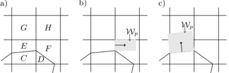
which is one of the fundamental steps in our algorithm devised in Section 3. Here q ∈ lRm denotes the vector of m conservative quantities, and f (q), g(q) denote the flux vectors, see (1) for an example. We will describe the method on a slightly nonuniform grid denoted by G that is composed of a set of regular cells with a fixed mesh spacing ∆x and ∆y in the x- and y-direction, respectively, and some irregular cells which are formed by inserting tracked boundaries into the grid, see Fig. 1a for an illustration.
We use a standard finite volume formulation of the method that the ap-proximate value of the cell average of the solution over any given cell S at time tn can be written as
QnS≈ 1 M(S) Z S q(x, y, tn) dx dy,
where M(S) is the measure (area) of this cell. The methods we use are based on solving one-dimensional Riemann problems at each cell edge, and the re-sulting waves (discontinuities moving at constant speeds) are employed to update the cell averages in the cells neighboring each edge (cf. [6]).
a) b) c) C E D F G H ↓ ↓ Wp Wp
Fig. 1. (a) A typical grid created by our algorithm. A wave propagating normally
from the cell edge: (b) between cells E and F updates the solution in cell F , and (c)
between cells C and E updates four neighboring cell averages. Here Wp represents
the region swept out by the p-wave over a time step ∆t, for p = 1, 2, · · · , m.
Consider the cell edge between irregular cells E and F as illustrated in Fig. 1a, for example. We solve the one-dimensional Riemann problem normal to this face, which in this case will be
∂q ∂t +
∂f (q) ∂x = 0, with the initial data given by Qn
Eand QnF. If Roe’s approximate solver (cf. [9])
is chosen to solve the Riemann problem, the jump Qn
F− QnE would be
decom-posed into eigenvectors of A which is a localization of the Jacobian matrix of f (q), Qn
F−QnE=
Pm
p=1αprp, where rpis the pth eigenvector of A, Arp= λprp
with λp the corresponding eigenvalue, and αp gives the wave strength.
Figure 1b shows a typical p-wave with λp > 0, where part of cell F is
affected by this wave over a time step ∆t. In the simplest first-order version of the wave-propagation method, this cell average is updated by
Qn+1 S := Q n+1 S − M (Wp∩ S) M(S) αprp (3)
for S = F . Here Wp represents the region swept out by the wave and αprp is
the jump across the wave. Note that we have employed a standard initializa-tion procedure, Qn+1S := Q
n
S, for all S.
Now, if we are concerned with the cell edge between cells C and E (this is one segment of the tracked moving object with its normal oriented towards the outside), a Riemann problem would be solved in the direction normal to this face with appropriate chosen data Qn
C and QnE that takes account of the
moving-boundary conditions on this face. Here the p-wave indicated in Fig. 1c overlaps four cells, and using (3) in a similar manner gives modification of the cell average in each of these cells by the jump across this wave, weighted by the fraction of the cell area covered by the wave.
Note that because waves are allowed to propagate through more than one grid cell and are not confined to stay within neighboring cells, this first-order method is typically stable as long as the time step ∆t satisfies the CFL (Courant-Friedrichs-Lewy) condition relative to the regular ∆x and ∆y,
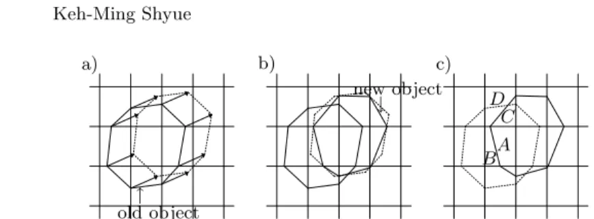
a) b) c) C D BA ↓ new object ↑ old object
Fig. 2. (a) With a given moving-object velocity at the current time, the tracked
interfaces are advanced in a Lagrangian manner over a time step ∆t. (b) Final location of tracked interfaces are set by where the new segments obtained in a) intersect the grid line. (c) Sample cases for the initialization of new irregular cells.
ν = ∆t max m p=1|λp| min(∆x, ∆y) ≤ 1 2, (4)
even when there are very small irregular cells near the tracked interfaces. To improve the stability condition of the method to ν ≤ 1 as well as the accuracy of the method to high resolution, it is straightforward to apply the techniques developed in [7] to the current instance.
3 Moving-Boundary Tracking Algorithm
In each time step, our moving-boundary tracking method for compressible fluid dynamics problems in two dimensions consists of the following steps: (1) With a given moving-object velocity at the current time, advance the
location of the tracked interfaces on the grid system Gn in a Lagrangian
manner over a time step ∆t, see Fig. 2a for an illustration.
(2) Find the new tracked-interface location using the result obtained in step 1, yielding the new grid system Gn+1, see Figs. 2b. Some cells will be
subdi-vided, and the values in each new irregular cell must be initialized. (3) Employ the finite volume wave-propagation method on the grid Gn+1
created in step 2 to update the cell averages of our physical model for single or multicomponent compressible flow over ∆t.
(4) Determine the new moving-object velocity at the next time step.
Note that steps 1 and 2 constitute the basic surface-moving procedure (cf. [7]) for the propagation of rigid object, step 3 is the construction of ap-proximate solutions to the physical problems of interests on a grid containing moving object, see Section 2, and step 4 is simply the calculation of the ve-locity for the moving object at the next time step.
Here the initialization of the irregular cell values is done by
Qn S := X χ∈Gn M (χ ∩ S) M(S) Q n χ (5)
for all S ∈ Gn+1, when the value Qn
χ is known a priori on Gn. As in many
existing moving-boundary methods (cf. [1, 5, 11]), an extrapolation procedure should be devised to assign state values that are in the interior region of the moving object, and incorporate that in (5) for the evaluation, see the cases for S = A, B, C, and D as illustrated in Fig. 2c. In the present work, we take an approach developed by Forrer and Berger [5] for that.
It should be mentioned that in case the motion of the object is induced by the flow field, such as the cylinder lift-off problem studied in Section 4, the velocity of the object (u, v)b at the time step tn+1can be computed based on
the Newton’s second law of motion by
(u, v)n+1b := (u, v) n b + ∆t Mb (Fx, Fy)nb,
where Mbis the mass of the object, and the vector (Fx, Fy)nb is the force on the
object which can be calculated by a numerical integration of the flow pressure times the normal vector along the surface of the object.
4 Numerical Examples
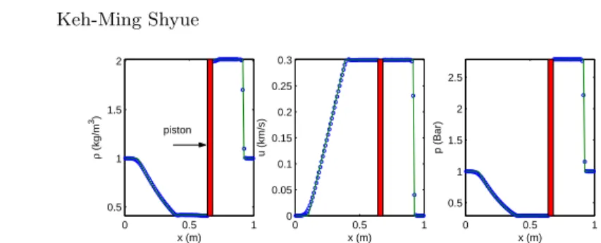
We now present sample numerical results obtained using our algorithm for compressible flow problems with moving geometries. Unless stated otherwise, we have done all the tests using a high-resolution wave-propagation method with the minmod limiter and the Courant number ν = 0.9 as defined in (4). Moreover, the material-dependent parameters in the equation of state (2) are set by (γ, B) = (1.4, 0) and (7, 3000Bar) for the gas- and liquid-phase, respectively. The boundary conditions of the computational domain are solid walls on the top and bottom, and non-reflecting outflow on the left and right. Example 4.1.We begin by considering a benchmark test that involves a one-dimensional piston moving at constant velocity in a two-dimensional domain. Initially, inside a shock tube with dimensions 1 × 0.2m2, we have a
piston of size: (x, y) ∈ [0.4, 0.44] × [0, 0.2]m2
, that is about to move vertically from left to right with a constant velocity (u, v)b= (0, 300)m/s into a region
of quiescent perfect gas with ρ = 1kg/m3
and p = 105
Pa. It is known that the exact solution of the problem would consist of a rightward-going shock wave in the front and a leftward-going rarefaction wave in the rear of the moving piston. In Fig. 3, we show the computed solution for the density, velocity in the x-direction, and pressure at time t = 800µ along the line y = 0.1m, using a 100 × 20 uniform grid. From the displayed profiles, it is clear that our numerical result is in good agreement with the exact solution.
Example 4.2.Our next example is concerned with the so-called cylinder lift-off problem (cf. [1, 3, 4, 5]) in which the Newton’s second law of motion is applied to model the movement of the moving object. In this problem, the initial condition consists of a planar Mach 3 shock wave in air located at x = 0.08m traveling from left to right (the pre-shock state is at rest with
0 0.5 1 0.5 1 1.5 2 x (m) ρ (kg/m 3) 0 0.5 1 0 0.05 0.1 0.15 0.2 0.25 0.3 x (m) u (km/s) 0 0.5 1 0.5 1 1.5 2 2.5 x (m) p (Bar) piston
Fig. 3. Cross-sectional plots of the density, x-component velocity, and pressure
for the one-dimensional moving piston problem at time t = 800µs along the line
y= 0.1m. The solid line is the exact solution.
density 1.4kg/m3 and pressure 1Pa), and a stationary rigid circular cylinder
(which has density 10.77kg/m3) with center (x
0, y0) = (0.15, 0.05)m and of
radius r0= 0.05m in front of the shock wave.
Figure 4 shows the contours of pressure at three different times, t = 0, 0.1641, and 0.33085s obtained using our method with a 1000 × 200 grid. From the figure, it is easy to notice the asymmetric reflection of the incident shock wave by the cylinder at the bottom side. When the time proceeds, the re-flected pressure would be higher near the bottom, causing the lift-off effect to the cylinder. In view of the global structure of the solution, our results agree quite well with the results displayed in [1]. In Table 1, we present a conver-gence study of the center of the cylinder and the relative mass loss at the final stopping time t = 0.30085s, observing a linear convergence on the latter quantity, when the mesh is refined. It should be noted that when comparing this results with the one appeared in [1], we see a slight difference on the center of the cylinder. More work should be done to clear up the discrepancy.
Table 1. A convergence study of the center of cylinder and the relative mass loss
for the cylinder lift-off problem at the final stopping time t = 0.30085s. Mesh size Center of cylinder (m) Relative mass loss
250 × 50 (0.618181, 0.134456) −0.257528
500 × 100 (0.620266, 0.136807) −0.131474
1000 × 200 (0.623075, 0.138929) −0.066984
Example 4.3.Finally, as an example to show how our algorithm performs for multicomponent problems with moving geometries, we are interested in the flying of a supersonic projectile into a partially-filled water container. Here we take a projectile with a circular shape of radius 0.3m, and consider a constant velocity motion (u, v)b= (0, −500)m/s of the projectile where its initial
0 0.1 0.2 0.3 0.4 0.5 0.6 0.7 0.8 0.9 1 0 0.05 0.1 0.15 0.2 0 0.1 0.2 0.3 0.4 0.5 0.6 0.7 0.8 0.9 1 0 0.05 0.1 0.15 0.2 0 0.1 0.2 0.3 0.4 0.5 0.6 0.7 0.8 0.9 1 0 0.05 0.1 0.15 0.2 t= 0 t= 0.1641s t= 0.30085s
Fig. 4. Contour plots of the pressure for the cylinder lift-off problem at three
different times t = 0, 0.1641, and 0.30085s by using a 1000 × 200 grid.
Above the horizontal air-water interface at y = 0, the fluid is a motionless air with the standard atmospheric condition, while below the interface the fluid is water at rest with density 1000kg/m3 and pressure 1Bar. The boundary
conditions on the computational domain are solid walls on the left, right, and bottom, and non-reflecting outflow on the top.
To solve this two-fluid problem numerically, our moving-boundary tracking algorithm uses a mixture type of the model equations proposed in [10] as the basis for approximation. Results of a sample run obtained using the algorithm with an uniform 600 × 600 grid are shown in Fig. 5 where contours of the density, pressure, and volume fraction are shown at three different times t = 1, 2, and 3ms. From the figure, it is interesting to see the time evolution of the air-water interface, upon the projectile entering the body of water. In the future, we plan to validate this result by making comparison with either the laboratory experiments or the ones obtained using other numerical methods.
References
1. M. Arienti, P. Hung, E. Morano, and J. E. Shepherd. A level-set approach to Eulerian-Lagrangian coupling. J. Comput. Phys., 185:213–251, 2003.
2. S. A. Bayyuk, K. G. Powell, and B. van Leer. An algorithm for simulation of flows with moving boundaries and fluid-structure interactions. AIAA paper CP-97-1771, 1997.
3. M.-H. Chung. A level set approach for computing solutions to inviscid com-pressible flow with moving solid boundary using fixed Cartesian grids. Int. J. Numer. Meth. Fluids, 36:373–389, 2001.
−2 0 2 −3 −2 −1 0 1 2 3 −2 0 2 −3 −2 −1 0 1 2 3 −2 0 2 −3 −2 −1 0 1 2 3
Density Pressure Volume fraction
air water t= 1ms −2 0 2 −3 −2 −1 0 1 2 3 −2 0 2 −3 −2 −1 0 1 2 3 −2 0 2 −3 −2 −1 0 1 2 3 air water t= 2ms −2 0 2 −3 −2 −1 0 1 2 3 −2 0 2 −3 −2 −1 0 1 2 3 −2 0 2 −3 −2 −1 0 1 2 3 air water t= 3ms
Fig. 5.Contours of the density, pressure, and volume fraction for a flying projectile
into water problem at three different times t = 1, 2, and 3ms. The dashed line is the initial location of the air-water interface, and the arrows are the computed velocities.
4. J. Falcovitz, G. Alfandary, and G. Hanoch. A two-dimensional conservation laws scheme for compressible flows with moving boundaries. J. Comput. Phys., 138:83–102, 1997.
5. H. Forrer and M. Berger. Flow simulations on Cartesian grids involving complex moving geometries. In Hyperbolic Problems: Theory, Numerics, Applications,
pages 315–324. Birkh¨auser-Verlag, 1999. Intl. Ser. of Numer. Math., Vol. 130.
6. R. J. LeVeque. High resolution finite volume methods on arbitrary grids via wave propagation. J. Comput. Phys., 78:36–63, 1988.
7. R. J. LeVeque and K.-M. Shyue. Two-dimensional front tracking based on high resolution wave propagation methods. J. Comput. Phys., 123:354–368, 1996. 8. S. M. Murman, M. J. Aftosmis, and J. Berger. Implicit approaches for moving
boundaries in a 3-D Cartesian method. AIAA-2003-1119.
9. P. L. Roe. Approximate Riemann solvers, parameter vector, and difference scheme. J. Comput. Phys., 43:357–372, 1981.
10. K.-M. Shyue. An efficient shock-capturing algorithm for compressible multi-component problems. J. Comput. Phys., 142:208–242, 1998.
11. G. Yang, D. M. Causon, D. M. Ingram, R. Saunders, and P. Batten. A Carte-sian cut cell method for compressible flows- Part B: moving body problems. Aeronaut. J, 101:57–65, 1997.