A neural network approach of input-output linearization of affine nonlinear systems

ProCItdlqi of b e Amdcm C o n h l Conlomneo

Balllmon, Maryland Juno 1954

FM7

=

2 1 0

A Neural Network Approach of

Input-Output Linearization of Affine Nonlinear

Systems

Wei-Song Lin, Hong-Yue Shue and Chi-Hsiang Wang Department of Electrical Engineering, National Taiwan University, Taiwan, R.O.C.

e-mail : weisong@mailbox.ee.ntu.edu.tw Abstract

For practical reasons, in the technique of feedback linearization, the requirements of mathematical modeling and access

of

internal states of complicated nonlinear systems should be removed. This paper demonstrates that, simply using output feedback, the input-output linearization of affine nonlinear systems with zero dynamics being exponentially stable can be accomplished by using multilayer neural network to estimate the instantaneous values of the nonlinear terms appearing in the feedback linearizing control law. Neither mathematical model nor internal state of the nonlinear system is required. The configuration for training the multilayer neural network as a device of the input-output linearizing controller is established. An example of affine nonlinear system is studied by computer simulations for various cases linearizing control.

1. Introduction

Feedback linearization based on concepts from differential geometry [2,6,9] can be adopted as a design methodology of nonlinear control systems. Using nonlinear coordinate transformation and feedback control, the original nonlinear model can usually be transformed into an equivalent linear one. With the terminology's, input-state and input-output linearizations refer respectively to complete [5,7,12] and partial linearizations [4,8,10].

For the linearized system, the well-developed design techniques of linear systems can be applied to solve for the appropriate controller. This approach has been successfully applied to a number of practical control plants such as high performance aircraft's, industrial robots and biomedical devices, Even though, there still exists major challenges for the feedback linearization design such as the requirement of precise mathematical model, the necessity of state feedback, and no guarantee of robustness in the appearance of parameter uncertainty or unmodeled dynamics [ 1 I].

Identifying the nonlinearity of control systems by neural networks through learning contributes another concept of nonlinear system design [I]. It is shown in this paper that, simply using output feedback and without the mathematical model of the system, the input-output linearization of an affine nonlinear system can be accomplished by estimating the decoupling matrix appearing in the approximated incermental linearizing control law with multilayer neural networks.

2. The Problem Of Neural-Network-Based Input-Output Linearization

Consider a square, affine nonlinear system with exponentially stable zero dynamics described by the following nonlinear differential equations

dynamics of a nonlinear system is the dynamics of the system when the outputs are constrained to be identically equal to zero.) For simplicity the arguments regarding to time, unless noticed, are omitted by the expressions in the following context. In the designs of input-output linearization, each output,

Y,,

of equation

(1)

is differentiated with respect to time repeatedly until at least one of the control inputs appears in the output equation. If r, represents the relative degree associated w t h Y,. Then the ("-order derivative of y , with respect to time can be written as follows :

where h, denotes the j I h component of h, L,h,(x): R"

-+

R and L,,h,(x): R "

-+

R stand for the Lie derivatives of h,(x) with

respect to f(x) and gJ(x), respectively. Equation (2) can be rewritten in vector-matrix form as follows

y'" = c(x)+ D(x)u (3)

where Y(') = [y!q), #),

. .

.,

J A ; ) ] ~ with r, ,r,

,. .

.,r,,, being the relative

degrees of the system, the decoupling matrix is

I

L&-'h,(x) * * . L&'h,(X)

[ -

L,, L;1.-'hlIl(x)

.. .

L,," Lf"h,,,( X ) D(x) = and c( x) = [L;

h,

(x),

.

.

.)

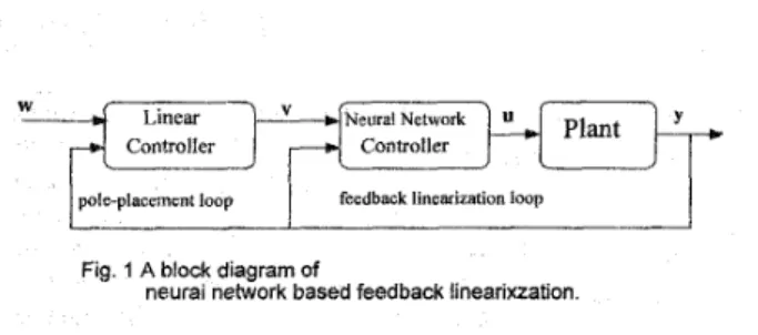
Lth,,(X)]'.

If the mathematical model of the nonlinear system is given, the design of input-output linearization is to solve for the control law, U, so that the closed-loop characteristics of the system characterized by equation (3) is linearized. Unfortunately the availability of mathematical model is not the practical case of most complicated nonlinear systems. For many real world applications, the mathematical models are usually severe difficult to be identified. This reality keeps the feedback linearization approach of many complicated nonlinear systems remaining in the theoretical phase. Instead of using the mathematical model, our consideration is to accommodate the nonlinearity required in the linearizing control law by the learning ability of artificial neural networks. Fig. 1 shows a block diagram of this substitutive configuration. Comparing with equation (3), the neural network may provide the estimations of nonlinear functions, D(x) and c(x). through an appropriate learning process. This configuration releases the designer from the necessity of mathematically modeling the nonlinear plants. The goal is to establish the design procedures and show the feasibility of neural-network-based input-output linearization of nonlinear systems. Only square, affine nonlinear systems with zero dynamics being exponentially stable are considered.

[L

L

F

-

H

F

T

Controller Controller feedback linearization loop

y-r-l

pleplaccment loop

Fig. 1 A block diagram of

neural network based feedback linearixzation

3. The Incremental Linearizing Control Law

If the decoupling matrix, D(x), of the nonlinear system characterized by (1) is nonsingular, the exact linearizing control law is

where v ER"' is the auxiliary input vector. Applying (4) to (3) yields the following m decoupled linear, SISO, systems

To stabilize the linearized system described by ( 5 ) , many well- developed linear design methods can be applied. Pole-placement by output feedback may give control laws as

for i=1,2, ..,m to achieve closed-loop characteristics governed by

U = D-'(x)[-c(x)+v] (4) V. ( 5 ) y(r) = v, = w, - a , l y ~ ~ - ~ ) - . . . - u l ~ ~ l ~ , - a , $ y I y,oi)+a,,yjr.-l)+

...+

u,,_,j,+a,,y, = w, (6) (7)

where w,qs are reference inputs, aI/Is, j=1,2 ,..., r are the parameters to be chosen so that SG

+a,,

sG-'+...+a,$ are Hurwitz polynomials.

For the nonlinear system under consideration is with c(x) and D(x) being uniformly continuous functions of time over the interval

o

I t I L . Then c(x),,,

+

c ( x ) ( ~ - ~ ) and D(x)(,)

-+

D(x)(,~-~) are true for sufficiently small sampling intervai of T = t, - tk-l, where 0 5 T 5 L and the subscripts denote the time instant at t,. This knowledge motivates the time-delay control law of input-output linearization as follows E1 31,

It has been shown that if one chooses an appropriate

fi

such that U ( k ) = D-'(x>(,)

K-Y;L)

+ D(X)(k-l) U(*-I)) + V(k)I (8)

(9) 111 - D( x)D-'

11

< 1

and further, keeps the auxiliary inputs, v, as uniformly continuous functions of time, where I represents an identity matrix with appropriate dimension. Then the system defined by (1) can be input-output linearized by applying the following approximated time-delay control law,

U(,) = D-WY;;!,) + DU(kbI))+ V(k)I (10) Here, using D(x)(,, = D(x)(~+ and after rearrangement of (8), we obtain the incremental linearizing control law as follows,

U@) = 0. Au(,) = ~ ( k )

-

U(,-,) = D-'(x)(k)[v(k)

-

Y&)], (11) Using multilayer neural nenvork 10 give the estimation of D(x)(,, as

6(k)

at every sampling instant, the approximation of the incremental linearizing control law is obtained as follows, In the digital realization of the linearizing controller, the uniformly continuous property of the auxiliary input is usually not guaranteed. Under this consideration, the following theorem shows the situations of the tracking error in applying the approximated incremental linearizing control law.

Theorem 1 Consider the nonlinear system and its controller being well defined by (1) and (12), respectively and c(x) and D(x)

AU(k) = U(k) -U(,-,) = D - l ( k ) [ V ( , )

-Y;;!l)l,

U@) = 0. (12)

(16)

W ( k )

- Y g I

=

P

-D(X)(k)D;kl)ltv(k-l)

- Y ; L ) l +

[I

-

D(x)(k)D;&k)

-

V(k-I)l

Taking norm on vectors and induced norm on matrices of equation (1 6), the following inequality is obvious

Since 2p 1, (20) depicts that the tracking error converges exponentially to zero for sufficiently large value of k.

case (iii)- When

IIv(~)

-

~ ( ~ - ~ ) l l >

I(v(~_~)

-

yi;$11

,

the substitution of IIv(,) -vg-,)1I for

]Iv(~-~)

--y{;!,)]] on the right side of (17), we obtain

IIv(k) -Y$ll'

2111-

D(x)(k)D~~)ll, IIv(k) -v(k-l)l] (21)

This proves the last case.+

For nonlinear systems being exactly linearized, the tracking error should always be kept at zero. However this is only possible when perfect model of the system is available. Alternatively, by using the approximated incremental linearizing control law, theorem 1 has revealed that if the decoupling matrix can be estimated accurately to some extent and the auxiliary input is manipulated finely. The tracking error of the linearizing control can either be constrained within a bound as in case (iii), or even converge exponentially to zero as in the cases of (i) and (ii). As a result, instead of (S), the imperfect input-output linearizing control results in a perturbed linear system described by

where

5

represents the vector of perturbation. For case (iii), the perturbation may be so large that the linearizing control being divergent, if the decoupling matrix and the step size of the

auxiliary inputs are not chosen appropriately. 4. Neural Network Based Linearization 4.1. Issues of The Multilayer Neural Networks

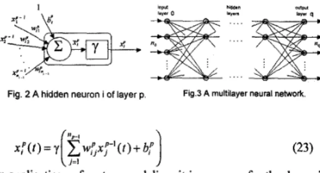
A neural network is a massively parallel, interconnected network of elementary units called neurons. A neural network with multiple neurons is usually organized into a sequence of layers, called multilayer neural network. The general structure of an (q+1) multilayer neural network with no inputs and n4 outputs can be illustrated as shown in Fig. 2 and Fig. 3. The input layer usually acts as

an

input data holder and signals flow from the input layer through the hidden layers to the output layer. The output of each neuron in the p f h layer can be expressed as

y'" = v

+ 5

₍₂₂₎

1

Fig. 2 A hidden neuron i of layer p. Fig.3 A multilayer neural network

(23) In applications of system modeling, it is common for the dynamic range of output data to be greater than 1, the activating function of the output node is therefore chosen to be linear. Thus the i*

output node performs a weighted s u m of its inputs as follows

4.2. Training of The Multilayer Neural Network for Input- Training of the neural network is to determine w's and

b's

such that x ; ( t ) of (24) is as close to the desired output as possible. Using Stone-Weierstrass theorem [3] it can be shown that a given nonlinear function under certain conditions can be represented by

Output Linearization

a corresponding series such as Voiterra series or Wiener series. The practical consequence of Stone-Weierstrass theorem is that an

infinitely large neural network can model arbitrary piecewise continuous function. A finite network, however, may only accurately model such functions over a subset of the domain. Our interest is mainly in networks which permit on-line identification and control of dynamic systems in terms of finite dimensional nonlinear differential equations.

The method commonly used to evaluate the gradient of a performance h c t i o n with respect to

a

weight vector of multilayer neural networks is called back propagation. If J(0) is the performance index which

has

to be optimized with respect to the parameter vector 6. Then

6

can be adjusted by according to the steepest decent method as the following equation

where 0 < q < 1, the step size, is a chosen parameter. In a multilayer neural network, the performance index

J

is usually chosen as

c(x,

-xP)' where are the desired values of ~ Y l s .

Thus

the weights and the thresholds are respectively updated according to

4

,=I

wPJ

( t ) = wP, (t - 1)

+

AwP, (t)

b,!( t ) = b,"( t

-

1)

+

Ab: (t)

with the increments AwP, (t) and Ab,! (t ) being given by Aw;(t) = q ,6p (t)X,P-' ( t )

+

IX~AW; (t

-

1)

Ab: (t ) = qb6

p

( t )

+

a,Ab," ( t

-

1) (27)

where the subscripts w and b represent the weight and threshold respectively, a, and ah are momentum constants, q, and qb

represent the learning rates and s p ( t ) is the error signal of the i'h

neuron of the p ' h layer. When the activating function of the output

neuron is linear, the error signal at

an

output node is and for the neurons in the hidden layer

s y ( 0

= X,(t)--XP(t) (28)

6; ( t ) = y (

Y

;

( t ) ) ! f 6 Y 1 (t)w;'( t

-

l), p = q

-

1,...,2,1 (29) ,=I

where y(K) denotes the first derivative of y(K) with respect to y.

To realize the estimations of nonlinear functions D(x) and c(x) in equation (3) for input-output linearizing control, Fig. 4 shows a configuration for training the multilayer neural network. In order to calculate the derivatives of plant outputs correctly, the training input u(t) are generated by sending sequences of random signals through digital lowpass filters with bandwidth

o

and sampling period T subject to the constraint o~ = 0.1 rad. The lowpass filter is of 2nd-order Butterworth type and can be expressed as

~ ( k )

= 1.8588~(k

-

1)

-

0.8681~(k

-

2)

(30)

+

0.00233(r(k)+ 2r(k -l)+ r(k

-

2))

where r(k) are random signals uniformly distributed in the operating range. The weights of the neural network are updated by using the steepest decent method represented by (27) with appropriate selections of the step size q and the momentum a to

minimize the performance index m

J = C(rjli'

-

j y ) *

,=I

where i?, and

Gv

are the elements of 2 and D, respectively, j f c ) is the ith component o f f ( " ) (the approximation of y(')) and r, is the

i s relative degree of the plant. Because the outputs of the neural network are 6 and D rather than

8'".

The error term described by (28) for the back propagation learning algorithm are modified to

s:,

= [y?

-

j!"]

,

for i = I,Z,.

.

.,m ₍₃₂₎

Sq di, - -[y,(';)-j!G)]uJ,fori=1,2

,...,

m and j = 1 , 2

,...,

m

where S z , S:g are the error signals for and

(ill,

respectively. The algorithms for training the weights of hidden layers of the neural network are kept unchanged. The most important thing of this training algorithm is that

-

L measurements of Backward Approximation

yq

outputs. This feature is practically necessary.

4.3. Estimation of Relative Degree

To obtain the form described by ( 3 ) for the design of input- output linearization, the knowledge of relative degrees is indispensable. This paragraph presents a numerically feasible method to determine the relative degrees of a nonlinear system.

Theorem 2 Assume that a nonlinear system characterized by equation (1) has continuous states and with relative degrees r,,r,,. .-,r,,,. Let the control input u,(t) associated with the relative degree of the irh output Y , be a piecewise continuous function with a discontinuity at t = t,, and u J ( t ) = 0 for all j + p of u(t). Then y , and its derivatives to the order of r,

-

1 are continuous

function of time, except that the order derivative, y(c), has a

discontinuity at t = t,.

proof : Differentiating the i l h output equation of system (1) up to

Fig. 4 The configuration for training the neural network

rl order, we have

yp' = c: ( x ) for k = O,l;..,r, -1; and (33)

(34) y? = c,? ( x )

+

d , ( x ) u

where c : ( x ) = L:ht(x) for

k

= O,l,.

.

.,rl, and

d , ( x ) = [L,,q-'h,(X) e * + LCmL:-'h,(x)] with L,,L:-'h,(X);t 0

are smooth functions of x. For continuous c,k(x) and from (33), we obtain

Similarly, from (34) and the continuity property of c,"(x) and

d , ( x ) , we achieve

y y ( t; )

-

y,'"( t; )

= L,,

q-'

h(x(ti ))[U, (t; ) -

= c,'(x(t; ))- C: ( ~ ( t ; ) ) + d,(x(j;))u(j:)-d,(x(t;))u(l;) (36)

( t i )] Z 0

Practically, to discover the relative degrees of a nonlinear system, one can drive the system with step or square wave inputs, then investigate the outputs and their derivatives for the appearances of discontinuities. The lowest order of the derivative of the ilh output which appears discontinuity corresponding to the jump or jumps

*

in any one input is the i'h relative degree of the system. A specid case of SISO systems is that the nonlinear function D(x) at the occurrence of discontinuity can be calculated from (36) as

(37) D(x(t,

1)

= [ ~ ' " ( t ; )

-

~ ( " ( t ; )I/[uCt;')

-

11

5. Simulation Results Given a third order system described by

Y = XI

where

exp(-x$)-l

c ( x ) = a x ,

+

8 exp(-x,/2)+1

D ( X ) = 4 - exp(-O.15x:

+

1.1)

A three-layer neural network (q=2) with 10 neurons in the hidden Iayer is adopted as the learning device of all the following simulations. The training algorithm updates the weights of the neural network by the steepest decent method and using step size q=O.Ol and momentum ~ ~ 0 . 0 1 .

case (a)- using fixed value for all

fi(k).

With a unit step input u ( t ) = u,(t), the value of D(x) at f = 0 can be estimated by using (37). The result is

I)

-

..

(39)

jj,+4yd+6y,=6w (40)

( 0 )

-

(Y(0' )

-

D-

) ) / ( U @ + ) - 4 0 -

1)

= (0.9957

-

0)/(1- 0 ) w 1

For the desired closed-loop dynamics being described by, the controller with the approximated incremental linearizing control is AU(k) = D ) ; i ) [ V ( k )

-

&k-i)l vck) = -4Y(k-i1 - ~ Y W + 6 w ~ (41) (42) where

Using

D,,,

= 1 for all time in (41), the simulation result is shown in Fig. 5 with the sampling period T = 0.01 sec., initial state

xo =[0.5 -1 O.2]', and w(*, = 1. Fig. 5 shows that the tracking of desired value, Y,, is in good quality. However, if w ( ~ ) = 4 , the feedback linearizing control system becomes unstable as shown in Fig. 6. This demonstrates the case (iii) of theorem 1.

case (b)- estimating D(x) on-line by neural network

Consider that the sequence of training input for the neural network is generated by sending the random signal r(k) uniformly distributed in the interval [-26, 341 through the lowpass filter (30) with sampling period T = 0.01 sec. ~ ( x ) is estimated by training the neural network for 30000 steps. Fig. 7(a) shows the satisfactory response of the system subject to the controller (40) even for w ( ~ , = 4 . Fig. 7(b) shows that D(k) is not precisely equal case (c)- effect of noise

To investigate the effect of noise on the approximated incremental linearizing control, a noise n ( t ) = 0.3sin(20t) is superposed on the output of the plant. Fig. 8 shows the output response of the system by using the control law

to D ( x ) ( k ) '

AU(k) = D&Y(k-I) + 40W(k) - lo&-I) - 40Y(k-,)l (43)

5

where

yk,

= ~ u , ( k T

-

i) and Dtk) is the estimation of D(x),,, being obtained by the neural network. The desired closed-loop characteristics is described by

The result depicts that the approximated incremental linearizing control can achieve good performance even in the presence of severe output noise.

1x0

ji,

+

1 Oy,

+

40y, = 40w (44)

6. Conclusion

Using output feedback and the learning ability of multilayer networks, it has been shown that the input-output linearization of affine nonlinear systems can be succeeded without mathematically modeling the nonlinear behavior. The configurations for the training and control of approximated exact and incremental linearizing control laws have been established. The incremental linearizing control is able to relax the tolerance of estimating error introduced by the neural network due to absence of internal states, disturbance of noise or inadequate capacity of the network itself. All the establishments are based upon that the affine nonlinear system being with exponentially stable zero dynamics. Given a nonlinear problem, there are still questions about what capacity of a neural network is necessary by the neural-network-based design left to be answered. As a conclusion, the approach with output feedback and neural learning has made feedback linearizing control more practical.

8 5

Acknowledgments - Financial support for this research .from National Science Council of Taiwan R. O.C. under MSC 82-0404- EOO2-259 is grate&& acknowledged

I

a

<

- ya

-

0 s 1 1 5 2 2 5

References

Bavarian, 3. (1988). Introduction to neural networks for intelligent control, IEEE Control Systems Magazine, 8,4, 3- 7.

Byrness, C. I., and A. Isidori (1985). Global feedback stabilization of nonlinear systems. Proceedings of the 24

IEEE CDC, Ft. Lauderdale, FL., 1031-1037.

Cotter, N. E. (1990). The Stone-Weierstrass theorem and its application to neural networks. IEEE Trans. Neural

Networks, 1,290-295.

Freund, E. (1975). The structure of decoupled nonlinear system. Int. J. Control, 21,443-450.

Hunt, L. R., R. Su, and G. Meyer (1983). Global transformations of nonlinear systems. IEEE Trans. autom.

Control, 28,24-3 I.

Isidori, A. (1989). Nonlinear Control Systems, 2nd Edition. Springer, New York.

Jakubczyk, B. and W. Respondek (1980). On linearization of control systems. Bull. Acad. Polon Sci. (Math.), 28, 517- 522.

Krener, A. J., and A. Isidori (1983). Linearization by output injection and nonlinear observer. Syst. Control Lett., 3, 47- 52.

Nijmeijer, H., and A. J. van der Schaft (1990). Nonlinear

Dynamical Control Systems. Springer. New York.

Porter, W. A. (1970). Diagonalization and inverses for nonlinear systems. Int. J. Control, 11,67-76.

Slotine, J.-J. E., and W. Li (1991). AppZied Nonlinear

Control. Prentice-Hall, Englewood Cliffs, NJ.

Su, R. (1982). On the linear equivalents of nonlinear systems. Syst. Control Lett., 2,48-52.

Youcef-Toumi, K., and S. T. Wu (1992). Input/output linearization using time delay control. ASME J: Dyn Syst.

andkfeas., 114, 10-19.

1 . 5

I

Fig. 5 Response when D,,, = 1, wl

Fig 6 Unstable results when fi,,, = 1, W 4

5 1

-

- -

- -

-

- - - -

_-

- - -

- -

:>

I

_ / - - - - 1 B E B S 3 . 5 I 5 3 (b ) Time(sec)

Fig 7 Stable results when estimating D(x) as fi,,,

fg 8 Response when disturbed by noise