A RECURRENCE METHOD FOR SIMPLE CONTINUOUS
LINEAR PROGRAMMING PROBLEMS
Ching-Feng Wen
*General Education Center
Kaohsiung Medical University
100, Shih-Chuan 1st Road, Kaohsiung, Taiwan, 807, R.O.C.
Yan-Kuen Wu and Yung-Yih Lur
Department of Industrial Management
Vanung University
ABSTRACT
In this paper, we discuss a special class of continuous linear programming problems which can be called simple continuous linear programming problems (SP). A practical and effi-cient method for finding an approximate optimal value and optimal solution of (SP) is pre-sented. The main work of computing an approximate optimal value in the provided method is only to solve finite linear programming problems by using recurrence relations. Further-more, a simple algorithm can be employed not only to easily solve the (SP) problem but also to provide an error bound of optimal value as well. Some numerical examples are given to implement the algorithm.
Keywords: continuous linear programming problems, recurrence method
1.
1INTRODUCTION
Continuous linear programming problems (CLP) proposed by Bellman [7, 8] in connection with the so-called bottleneck problems in multistage linear production processes, which are formulated as fol-lows: (CLP) : 0 maximize
∫
Tf t x t dt( ) ( ) 0 subject to ( ) ( ) ( , ) ( ) ( ), ( ) 0, [0, ], t B t x t K s t x s ds g t x t t T +∫ ≤ ≥ ∈where B t( ), K(s, t) are given m n× matrices, f t( )
is a given n-vector, g t( ) is a given m-vector and
( )
x t is an n-vector to be determined. Here all vectors are column vectors. In the literature, much research has been proposed to consider continuous linear pro-gramming problems. Studies on investigating a solu-tion algorithm for (CLP), [9, 10, 14, 16, 24] provided a generation of the simplex method to a function space setting. Considering the duality of (CLP), [12, 13, 17, 25, 26] established strong duality theorems. Also, Ho-Lur-Wu [15] studied extreme points of the feasible region for a special class of continuous linear programming problem. Studying a special case of (CLP), Anderson [1] introduced the separated con-tinuous linear programs (SCLP) to model job-shop scheduling problems. Since then many researches concerned with (CLP) has focused on (SCLP) [2, 4-6,
*Corresponding author: [email protected]
11, 18-23, 27]. One of a practical example of bottle-neck problems is described as follows [3].
In an economy, n different goods, G1, G2, . . . , Gn, are produced by m different types of plan or
pro-duction facility, P1, P2, . . . ,Pm. At the beginning of a
five-year plan, there is available a certain capacity in each of these types of plant, and more can be made by reinvesting the goods produced. The aim of the plan is to maximize the productive capacity at the end of the period.
Let xj(t), j = 1, 2, . . . ,m, denote the rate of
production of new capacity of type j at time t. Pro-duction of new plant requires the consumption of a certain quantity bij of good Gi for each additional unit
of plan Pj. Thus the amounts of goods consumed in
this way are given by Bx(t), where x(t) is the vector with components x1(t), x2(t), . . . , xm(t) and B is the
matrix whose i, jth element is bij . Let zj(t) denote the
total productive capacity of type j available at time t. Denote by dij the rate of production of Gi for each unit
of plant Pj . Then the total rates of production of
goods at time t are given by Dz(t), where D is the matrix whose i, jth element is dij and z(t) is the vector
(z1(t), z2(t), . . . , zm(t))T .
The constraint on investment in additional plant due to limitations in productive capacity is then given by Bx t( )≤Dz t( ) throughout the time period
under consideration. If c0 is the vector of initial pro-ductive capacities, we can write
0 0
( ) t ( ) ,
0
( ) t ( ) ,
Bx t −
∫
Dx s ds c≤ where c Dc= 0. If we wish tomaximize a weighted sum, ∑a z Ti i( ), of the
pro-duction capacities at the end of the time period, then we obtain the following linear program
maximize 0 ( ) T T a x t dt
∫
subject to 0 ( ) t ( ) , Bx t −∫
Dx s ds c≤ ( ) 0, [0, ]. x t ≥ t∈ TIn this paper we discuss a special case of con-tinuous linear programming problems. This continu-ous linear programming problem is defined as fol-lows: (SP): maximize 0 ( ) ( ) T f t x t dt
∫
subject to 0 ( ) t ( ) ( ), [0, ] x t −∫
x s ds≤g t ∀ ∈t T ( ) [0, ], x t L+ T ∞ ∈where f and g are continuous functions on [0,T] and
[0, ]
L+ T
∞
is the set of nonnegative real valued,
Lebesgue measurable, essentially bounded functions on [0,T]. The dual problem (DSP) of (SP) is defined as follows: (DSP): maximize 0 ( ) ( ) T g t w t dt
∫
subject to ( ) T ( ) ( ), [0, ] t w t −∫
w s ds≥ f t ∀ ∈t T ( ) [0, ]. w t ∈ ∞L+ TIt is well known that (SP) and (DSP) have the weak duality property (see, for example [3]), that is, if x(t) and w(t) are feasible for (SP) and (DSP) re-spectively, then 0 ( ) ( ) T f t x t dt≤
∫
0 ( ) ( ) . T g t w t dt∫
In-deed, the (SP) problem we studied is a special case of Tyndall’s work [25], which is an application to a dy-namic closed end Leontief production model. By Theorem 1 of [25] there exist optimal solutions x(t) and w(t) in (SP) and (DSP) respectively such that
0 ( ) ( ) 0 ( ) ( ) .
T T
f t x t dt= g t w t dt
∫
∫
However, Tyndall’swork only verified the theoretical result of optimal solution. It seems too complex to find the optimal solution in the work of computation. Motivated by this factor, we intend to present an efficient algorithm to approach the optimal value of (SP) by using recur-rence method. This method can be employed not only to easily solve the (SP) problem but also to provide an error bound of optimal value as well. For improv-ing the readability, we define the notations F(P) and V(P) to be the feasible region and the optimal value of a linear programming problem (P), respectively. For example, F(SP) is the feasible region and V(SP) is the optimal value of (SP).
This paper is organized as follows. In Section 2, a discretization method is prepared for the proof of the main theorem in the following sections. Applying this discretization method we can obtain a sequence
of optimal solutions of corresponding finite linear programming problems in Section 3. Then the corre-sponding value obtained from this sequence finally converges to the optimal value of (SP). In Section 4, we establish an error bound for the provided method and give some examples to illustrate the convergence of problem. Brief conclusion is given in Section 5.
2. PRELIMINARY RESULTS
For solving the (SP) and (DSP) problems, we use a discretization method for two functions f and g. For each n N∈ , let
2 1 2 2 1 {0, , , , 2 2 2 n n n n n P = T T … − T
, }T
be a partition on [0,T]. For i = 1, 2,… , 2n, let
( ) min{ ( ) : [ 1 , ]} 2 2 n i n n i i b = g x x∈ − T T (1) and ( ) min{ ( ) : [ 1 , ]}. 2 2 n i n n i i c = f x x∈ − T T (2)
Step functions f tn( ) and g tn( ) are defined as
fol-lows: ( ) ( ) 2 1 , for [ , ), 2 2 ( ) , for , n i n n n n n i i c t T T f t c t T − ⎧ ∈ ⎪ = ⎨ ⎪ = ⎩ (3) and ( ) ( ) 2 1 , for [ , ), 2 2 ( ) , for . n i n n n n n i i b t T T g t b t T − ⎧ ∈ ⎪ = ⎨ ⎪ = ⎩
(4)
Consider the following programming problem: (SPn) : 0 maximize
∫
Tf t x t dtn( ) ( ) 0 subject to ( ) ( ) ( ), [0, ] ( ) [0, ], t n x t x s ds g t t T x t L+ T ∞ − ≤ ∀ ∈ ∈∫
and its dual problem:
0 ( ): minimize ( ) ( ) subject to ( ) ( ) ( ), [0, ] ( ) [0, ]. T n n T n t DSP g t w t dt w t w s ds f t t T w t L+ T ∞ − ≥ ∀ ∈ ∈
∫
∫
Assumption 1. f and g are continuous on [0,T], and g(t) > 0 for all t∈[0, T].
In this article, we always employ Assumption 1 to solve the continuous linear programming problems
(SP) and (DSP). Note that, under Assumption 1, we have the following properties.
(1) (SP) and (SPn) are feasible for all n∈N, since the
zero function is a common feasible solution of (SP) and (SPn). Moreover, let *( )
T t w t ke − , where [0, ] maxt T{ ( ), 0}. k= ∈ f t Then *( ) *( ) T t w t −
∫
w s ds k= ( ) n( ), f t f t≥ ≥ for all t
∈
[0, T]. Hence w*(t) is a common feasible solution of (DSP) and (DSPn) for alln∈N. Therefore, (SP), (DSP), (SPn) and (DSPn) are
all feasible.
(2) Since g1(t)
≤
g2(t)≤
···≤
g(t) and f1(t)≤
f2(t)≤
···≤
f t( ) for all t∈[0, T], we have1 2 ( ) ( ) ( ) F SP ⊆F SP ⊆ ⊆F SP and 1 2 ( ) ( ) ( ), F DSP ⊇F DSP ⊇ ⊇F DSP which implies −∞<V(SP1)≤ V(SP2)≤ ··· ≤ V(SP)<∞ (5) and −∞<V(DSP1)≤ V(DSP2)≤ ··· ≤ V(DSP) <∞. Hence, lim n→∞V(SPn)≤ V(SP) and lim n→∞(DSPn)≤ V(DSP). (6) Lemma 1. Suppose that Assumption 1 holds.
Let ( )n( ) w t be a feasible solution of (DSPn), [0, ] supt T{ ( )f t f tn( )} ε= ∈ − and [0, ] supt T{ ( )g t g tn( )} ε′ = ∈ − . Let ( )n ( ) ( )n ( ) w t =w t +εeT t− . Then w( )n ( ) t is a
fea-sible solution of (DSP) and
( ) ( ) 0 0 ( ) 0 0 0 ( ) ( ) ( ) ( ) ( ) ( ) . T n T n n T n T T t g t w t dt g t w t dt w t dt g t e dt ε ε − ≤ − ′ ≤ +
∫
∫
∫
∫
Proof. Observe that w( )n( )t ≥w( )n ( ) 0t ≥ and
( ) ( ) ( ) ( ) ( ) ( ) ( ) ( ) ( ) ( ) ( ) ( ) ( ) ( ) for all [0, ]. T n n t T T n T t n T s t t T n n t n w t w s ds w t e w s ds e ds w t w s ds f t f t t T ε ε ε ε − − − = + − − = − + ≥ + ≥ ∈
∫
∫
∫
∫
Hence w( )n( )t ∈F(DSP). Since w( )n ( )t ≥w( )n ( )t ≥0 and g t( )≥g tn( ) 0≥ , we have ( ) ( ) 0 0 ( ) 0 0 ( ) 0 0 0 ( ) ( ) ( ) ( ) [ ( ) ( )] ( ) ( ) ( ) ( ) . T n T n n T n T T t n T n T T t g t w t dt g t w t dt g t g t w t dt g t e dt w t dt g t e dt ε ε ε − − ≤ − = − + ′ ≤ +∫
∫
∫
∫
∫
∫
Based on Lemma 1, the optimal value of (DSP) can be obtained as the following theorem.
Theorem 1. Under Assumption 1, we have
lim
n→∞V(DSPn) = V(DSP).
Proof. Let ε > 0 be given. By continuity of f and g, there exists a positive integer N such that for all n
≥
N( ) ( ) ( )
n n
f t ≤ f t ≤ f t +ε and g tn( )≤g t( )≤g tn( )+ε,
for all t∈[0,T]. Here f tn( ) and g tn( ) are defined
as in (3) and (4). Let
w t
0( )
be a feasible solution of (DSP) and 0 0( ) .T
w t dt=θ
∫
For this ε > 0, we claim that for all n≥
N there exists w( )n( )t ∈F(DSPn) such that ( ) 0 0 T ( ) n( ) ( ) n n g t w t dt V DSP ε ≤
∫
− ≤ (7) and ( ) 0 ( ) , T n M w t dt mθ ≤∫
(8) where M =maxt∈[0, ]T g(t) and m =mint∈[0, ]T g(t). Weprove this claim by distinguishing the following two cases. Case 1. 0 ( ) ( )0 ( ) T n n g t w t dt V DSP− ≤ε
∫
. Put w( )n ( )t = 0( )w t . Then (7) holds and
( ) 0 0 ( ) 0 ( ) . T n T M w t dt w t dt m θ θ = = ≤
∫
∫
Case2. 0 ( ) ( )0 ( ) . T n n g t w t dt V DSP− >ε∫
Then there exists ( )n( ) ( ) n w t ∈F DSP such that ( ) 0 0 0 ( ) T ( ) n ( ) T ( ) ( ) n n n V DSP ≤∫
g t w t dt≤∫
g t w t dt (9) and ( ) 0 ( ) ( ) ( ) . T n n n g t w t dt V DSP− ≤ε∫
Suppose that ( ) 0 ( ) . T n M w t dt mθ >∫
As g tn( )≥m
for all t, we have ( ) 0 ( ) ( ) T n n M g t w t dt m M mθ θ > =∫
0 0 0 ( ) 0 ( ) ( ) , T T n M w t dt g t w t dt =∫
≥∫
which contradicts (9),
hence ( ) 0 ( ) . T n M w t dt m θ ≤
∫
Therefore, (7) and (8) hold. Now for n ≥ N we define a function( )n ( ) ( )n ( ) T t
w t =w t +εe − for all t∈[0, T]. By Lemma
1, w( )n
is a feasible solution of (DSP) and
( ) ( ) 0 0 ( ) 0 0 0 0 ( ) ( ) ( ) ( ) [ ( ) ( ) ] [ ( ) ], T n T n n T n T T t T T t g t w t dt g t w t dt w t dt g t e dt M g t e dt m ε ε θ − − ≤ − ≤ + ≤ +
∫
∫
∫
∫
∫
(10)by (8). Moreover, observe that
( ) 0 ( ) ( ) 0 0 ( ) 0 0 0 ( ) ( ) ( ) ( ) ( ) ( ) ( ) ( ) ( ) ( ) [ ( ) ] , T n n T n T n n T n n n T T t g t w t dt V DSP g t w t dt g t w t dt g t w t dt V DSP M g t e dt m ε θ − ε ≤ − = − + − ≤ + +
∫
∫
∫
∫
∫
by (7) and (10). Since ε is arbitrary,
( ) 0
lim T ( ) n( ) lim ( )
n
n→∞
∫
g t w t dt=n→∞V VSP . Owing to the factthat ( ) 0 ( ) ( ) ( ), T n g t w t dt V DSP≥
∫
we obtain lim ( n) ( ).n→∞V DSP ≥V DSP Applying this result and (6),
we have lim (n→∞V DSPn)=V DSP( ). This completes the
proof.
3. A RECURRENCE METHOD
FOR (SP)
In this section we discuss the finite dimen-sional linear programming problem (Pn) which is due
to (SP). A recurrence method is then provided for solving the dual problem of (Pn) and verifying the
optimal value of (Pn) is just to the approximate
opti-mal value of (SP).
For each n∈N, let ( )n i
b and ( )n i
c be defined as in (1) and (2). Note that under Assumption 1, we have ( )n
i
b > 0 for all i. Now we define the following linear programming problem:
( ) 2 1 ( ) 1 1 ( ) 2 2 2 ( ) : maximize 2 1 0 subject to 1 0, 1,..., 2 . n n i i n n i n n T n n n i Tc x P x b x b i x = − ⎡ ⎤⎡ ⎤ ⎡ ⎤ ⎢ ⎥⎢ ⎥ ≤⎢ ⎥ ⎢ ⎥⎢ ⎥ ⎢ ⎥ ⎢ ⎥⎢ ⎥⎣ ⎦ ⎢ ⎥ ⎣ ⎦ ⎣ ⎦ ≥ ∀ =
∑
It is easy to see that the zero vector is a feasible solution of (Pn) and the dual problem (Dn) of (Pn) is
defined as follows: ( ) 2 1 ( ) 2 1 1 ( ) 2 2 ( ) : minimize 2 1 subject to 0 1 0, 1,..., 2 . n n i i n n i T n n n n n n i Tb w D w c w c w i = − ⎡ ⎤ ⎡ ⎤ ⎡ ⎤ ⎢ ⎥ ⎢ ⎥ ⎢ ⎥ ≥ ⎢ ⎥ ⎢ ⎥ ⎢ ⎥ ⎢ ⎥ ⎢ ⎥ ⎢ ⎥ ⎢ ⎥⎣ ⎦ ⎣ ⎦ ⎣ ⎦ ≥ ∀ =
∑
Remark 1. Under Assumption 1, it is easy to obtain an optimal solution of (Dn) via the following
recur-rence method; hence, through the strong duality the-ory of finite linear programming we have −
∞
< V(Pn)= V(Dn) <∞. To find an optimal solution of (Dn), let
( )n
w
= ( ) ( ) 1 2 ( n ,..., n )T n w w , where ( ) ( ) 2 max{ 2 , 0} n n n n w = c and 2 ( ) ( ) ( ) 1 1 max{ ,0}, 1, 2,..., 2 1. 2 n n n n n i n l i T w c w i = + = +∑
= −It is obvious that
w
( )n is a feasible solution of (Dn).Now we show that w( )n is an optimal solution of
(Dn). Let ( ,1 2,..., 2 ) ( ) T n n w= w w w ∈F D be given. Clearly, ( ) ( ) 2 max{ 2 , 0} 2 . n n n n n w ≥ c =w We claim ( )n k k
w ≥w for all k = 1, 2, . . .2n, and prove it by
in-duction. Suppose that ( )n
j j
w ≥w for all j = k +1, k + 2, . . . , 2n. Since w
is a feasible solution, we have
2 T k n w ≥ ( ) 1 2 2 ( n) n k k k w+ +w+ + +w +c . Thus, ( ) 1 2 2 ( ) ( ) ( ) ( ) 1 2 2 ( ) max{ ( ),0} 2 max{ ( ),0} 2 = . n k k n k k n n n n n k n k k n n k T w c w w w T c w w w w + + + + ≥ + + + + ≥ + + + +
Therefore, ( )n k k
w ≥w for all k = 1, 2, . . . 2n. This
proves the claim. Applying Assumption 1, ( )n 0 i
b >
for all i; hence, 2 ( ) 1 2 n T n i= nb wi i
∑
2 ( ) ( ) 1 2 . n T n n i= nb wi i ≥∑
Since w F D∈ ( n) is arbitrary, we see that( )n
w
is an optimal solution of (Dn).After the discussion of optimal solution for (Pn) and (Dn) problems, the optimal values of
rela-tionship between V(SPn) and V(Pn) are considered as
follows.
Theorem 2. Suppose that Assumption 1 holds. Then V(SPn)
≥
V(Pn), for all n = 1, 2, . . .. Proof. Let x=( ,...,1 2 ) T n x x be an optimal solution of (Pn). Define x(t) by ( 1) i 2 2 2 , for , 1, 2,..., 2 ( )= , for . i T iT n n n n x t i x t x t T − ⎧ ≤ < = ⎪ ⎨ = ⎪⎩ Case 1. ( 1) 2 2 [i T, ),iT n n t∈ − where 1≤
i≤
2n. Then0 1 ( 1) 1 2 1 ( ) 1 ( ) ( ) ( ) 2 ( ). 2 t i t i T i n j n j i n i n j i n j x t x s ds T x x x s ds T x x b g t − − = − = − = − − ≤ − ≤ ≤
∫
∑
∫
∑
Case 2. t = T. Then 2 2 0 1 2 1 ( ) 2 2 1 ( ) ( ) 2 ( ). 2 n T n n i i n n n n i n n i T x T x s ds x x T x x b g T = − = − = − ≤ − ≤ ≤∑
∫
∑
By case 1 and case 2, x(t) is a feasible solution for (SPn). It is easy to see that
2 ( ) 0 1 ( ) ( ) ( ). 2 n T n n n i i n i T f t x t dt c x V P = =
∑
=∫
Therefore, V(SPn)
≥
V(Pn). This completes the proof.According to Theorem 2, one can easy to see that V(DSPn)
≥
V(SPn)≥
V(Pn)=V(Dn). That isV(DSPn)
≥
V(Dn), for all n=1,2,… (11) By inequality (5) and Theorem 2, one can easily see thatV(DSP)
≥
V(SP)≥
V(SPn)≥
V(Pn)=V(Dn),for all n=1,2,…. (12) Theorem 3. Suppose that Assumption 1 holds. Then lim ( n) lim ( n). n→∞V D =n→∞V DSP Proof. Let ( ) ( 1( ),..., ( )2 ) n n n T n w = w w , as given in Remark 1, be an optimal solution of (Dn). Define a function
ˆ( ) w t by ( ) 1 2 2 2 ( ) 2 2 , for , 1, 2,...2 ˆ , for , n T t i i n i n n n n n n w e T t T i w w t T δ δ − − ⎧ + ≤ ≤ = ⎪ = ⎨ + = ⎪⎩ (13) where ( ) 2 max{2 : 1, , 2 }. n n T n nwj j δ = = … We first
show that w tˆ( )∈F(DSPn). For t∈[ 1 2 ,2 i i nT nT − ), we have 2 2 2 1 1 2 ˆ( ) ˆ( ) ˆ( ) [ ˆ( ) ˆ( ) ] T t j n iT T n n j t j i T n w t w s ds w t w s ds − w s ds = + − = − +
∫
∑
∫
∫
( ) ( ) 2 2 2 2 2 2 ( ) 2 1 2 1 1 2 ( ) [ ( ) ] 2 i T n T t n i n T s i n i n t n n n i T n n T s j j n n T j i j i n w e w T t e ds T w e ds δ δ δ − − − − = + = + = + − − + + +∫
∑
∑ ∫
2 ( ) ( ) ( ) 2 (2 ) 12 2 (1 ) n n T t n i T n T t i n i n n j n j i w δ e − w T t w δ e− = + = + − − −∑
+ − 2 ( ) ( ) ( ) 2 1 2 ( ) ( ) ( ) 2 2 1 2 ( ) ( ) ( ) 2 2 1 ( ) ( ) 2 2 2 (Since ) 2 ( ). n n n n i n j i n n j i n n T n n i n j n i n j i n n T n n i n j n n i j i n i n T i w w w T t T w w w T w w w c f t δ δ δ = + = + = + = − − − + ≥ − − + ≥ − ≥ ≥ =∑
∑
∑
Also, it is clear that
( ) ( ) 2 2 2 ˆ( ) T ˆ( ) ˆ n n ( ), n n n n T w T −
∫
w s ds w= +δ ≥c = f T hence ˆ( )w t is a feasible solution of (DSPn). Moreover,
observe that 2 ( ) ( ) 2 0 0 1 2 ( ) ( ) 2 0 1 2 0 ˆ ( ) ( ) ( ) 2 ( ) 2 ( ) ( ) . n T n n T T t n i n i n n i n T n n T t i n i n i T T t n n T g t w t dt b w g t e dt T b w g t e dt V D g t e dt δ δ δ − = − = − = + ≤ + = +
∑
∫
∫
∑
∫
∫
This and (11) together imply that
V(Dn)
≤
V(DSPn)≤
V(Dn)+ 2 0 ( ) . T T t n g t e dt δ −∫
(14) We now claim that2n
δ →0 as n→∞. To prove this claim, we need to prove the following fact by induc-tion: ( ) 2 (1 2 ) n j n j n T w L − ≤ + , for all 0,1,2, ,2 1 n j= … − ,
where L=max0≤ ≤t T{ ( ), 0}.f t Note that
( ) 1 2 max { n , 0} . n i i c L ≤ ≤ ≤ It is obvious that ( ) 2 n n w = ( ) 2 max{ n , 0} n c ≤L and ( ) ( ) ( ) 2 1 2 1 2 ( ) ( ) 2 1 2 max{ , 0} 2 max{ , 0} (1 ) . 2 2 2 n n n n n n n n n n n n n n T w c w T T T c w L L L − − − = + ≤ + ≤ + = + Suppose that ( ) 2 (1 2 ) n k n k n T w − ≤ + L, for all k=0,1,2, ,… j−1. Then
1 ( ) ( ) ( ) 2 2 1 2 0 1 ( ) ( ) 2 1 2 0 1 0 max{ , } 2 max{ , } 2 ( ) 2 2 ( ) 2
0
0
1
1
.
j n n n n j n n n k k j n n n n n k k j k n n k j n T w w T w T T Tc
c
L
L
L
− − − = − − − = − − = = + ≤ + ≤ + + = +∑
∑
∑
This proves the fact, which implies
( ) (1 )2 (1 )2 2 2 n n n j T j n n T T w ≤ + − L≤ + L e L≤ , for all 0,1, 2, , 2n 1. j= … − Thus, ( ) 2 1 2 0 max{ } . 2 2 n T n n n j n j T w T e L δ ≤ ≤ ≤ = ≤ Hence, 2n δ →0 as n→∞.
This proves the claim. Applying (14), (15), and Theorem 2, we see that lim ( n) lim ( n)
n→∞V D =n→∞V DSP .
This completes the proof.
By inequality (12), Theorem 3 and Theorem 1, we have V DSP( )≥V SP( ) lim (≥n→∞V Dn)=V DSP( )
.
Therefore, ( ) ( ) lim ( n), n V DSP V SP V D →∞ = = so wehave the following theorem.
Theorem 4. Suppose that Assumption 1 holds. Then V(DSP)=V(SP)=lim
n→∞V(Dn); that is, there is no duality
gap between (SP) and (DSP).
4. THE SOLUTION ALGORITHM
In this section, we discuss an error bound be-tween V(DSP) and V(Dn). An algorithm to approach
the optimal value of (SP) is established as well. Let
( ) ( ) ( ) 1 2 ( ,..., ) n n n T n w = w w be an optimal solution of (Dn)
as given in Remark 1. Let
2n max δ = ( ) 2 {T n : 1,...2 },n j n w j= ε =supt∈[0, ]T { ( )f t −f tn( )},
and ε′ =supt∈[0, ]T { ( )g t −g tn( )}. Then we have the
following result.
Theorem 5. Suppose that Assumption 1 holds. Then
0≤V DSP( )−V D( n)≤εn, where 2 ( ) 12 2 2 0 [ n T n ( T 1)] ( ) T ( ) T t . n i nwi n e n g t e dt ε ε δ ε δ − = ′ =
∑
+ − + +∫
Proof. Let ( ) ( ) ( ) 1 2 ( ,..., ) n n n T n w = w w be an optimal solu-tion of (Dn) and w t be defined as in (13). ˆ ( )( )nThrough the proof of Theorem 3, we see that ˆ ( )( )n
w t is a feasible solution for (DSPn), and
( ) 0 ( )ˆ ( ) ( ) 2 0 ( ) . T T n T t n n n g t w t dt V D≤ +δ g t e −dt
∫
∫
Let ( )n( ) ˆ( )n( ) T t w t =w t +εe− . By Lemma 1, w( )n ( )t is afeasible solution of (DSP) and
( ) ( ) 0 0 ( ) 0 0 2 ( ) 2 1 0 2 0 1 2 ˆ 0 ( ) ( ) ( ) ( ) ˆ ( ) ( ) ( ) ( ) T n T n n T n T T t n i T T T n n T t T t i n i T n i g t w t dt g t w t dt w t dt g t e dt w dt e dt g t e dt ε ε ε δ ε − − − − = ≤ − ′ ≤ + ′ = + +
∫
∫
∫
∫
∑∫
∫
∫
2 ( ) 2 0 1 [ ( 1)] ( ) . 2 n T n T T t i n n i T w e g t e dt ε δ ε − = ′ =∑
+ − +∫
Thus, ( ) 0 ( ) ( ) 0 0 ( ) 0 2 ( ) 2 2 0 1 0 ( ) ( ) ( ) ( ) ( ) ˆ ( ) ( ) ( ) ( ) ˆ ( ) ( ) ( ) [ ( 1)] ( ) ( ) . 2 n T n n T n T n n T n n n n T n T T t i n n n i V DSP V D g t w t dt V D g t w t dt g t w t dt g t w t dt V D T w e g t e dt ε δ ε δ − = ≤ − ≤ − = − + − ′ ≤ + − + +∫
∫
∫
∫
∑
∫
This completes the proof.
According to Theorems 4 and 5, we summarize the preceding discussions to form the following pro-cedure for finding the approximate optimal value of (SP).
Algorithm:
Let δ be a prescribed small positive number, and an initial number n0∈N be given.
Step 1. Set n
←
n0. Step 2. Calculate( )n i
w for i=1, 2, , 2… n by the
re-currence method as in Remark 1. Evaluate the error bound ε as defined in Theorem 5. n
Step3. If εn≤δ , then stop and evaluate the value 2 ( ) ( )
12
n n n
i= T b wn i i
∑
as the approximate value of this problem. Otherwise, update n←n + 1 and go to Step 2.Remark 2. From Theorem 4, we can approach the value V(SP) by V(Dn). Note that by the
complemen-tary slackness theorem of finite linear programming, we can via the optimal solution w( )n of (D
n) to
ob-tain an optimal solution of (Pn), say ( ) ( ) ( ) 1 2 ( ,..., n ) . n n n T x = x x Definex( )n( )t by ( ) 1 2 2 ( ) ( ) 2 , if [ , ), 1, 2,..., 2 ( ) , if . n i i n i n n n n n x t T T i x t x t T − ⎧ ∈ = ⎪ = ⎨ = ⎪⎩
Applying the same argument as the proof of Theorem 2, we see that ( )n ( ) ( ) n x t ∈F SP (hence ( )n ( ) ( ) x t ∈F SP ) and ( ) 0 ( ) ( ) ( ) T n n n f t x t dt V P=
∫
. Since ( ) ( ) n f t ≤ f t , by Theorem 5, we have( ) 0 ( ) 0 0 ( ) ( ) ( ) ( ) ( ) ( ) , T n T n n n V SP f t x t dt V SP f t x t dt ε ≤ − ≤ − ≤
∫
∫
where ε is defined as in Theorem 5. Therefore, the n value ( )
0 ( ) ( )
T n
f t x t dt
∫
is an approximate value of (SP), and the error between the optimal value and the approximate value is less or equal to ε . nFor illustration purpose, we use two examples to show that the proposed scheme works for real. Example 1. 1 3 0 0 maximize ( 4 1) ( ) subject to ( ) ( ) 1, [0,1] ( ) [0,1]. t t t x t dt x t x s ds t t x t L+ ∞ − + − ≤ + ∀ ∈ ∈
∫
∫
Example 2. 1 2 0 0 maximize sin(7 ) ( ) subject to ( ) ( ) 2 cos(5 ), [0,1] ( ) [0,1]. t t t x t dt x t x s ds t t x t L+ ∞ − ≤ + ∀ ∈ ∈∫
∫
To illustrate the convergence, we select the partition number n from 1 to 20 and put ( )n min{ ( ) :
i c = f x x∈[ 1 2 ,2 i i n n − ]} and ( ) 1 2 2 min{ ( ) : [ , ]},n n n i i i b = g x x∈ − for all i=1, 2, , 2… n. Using MATLAB Version 7.0.1 on
a PC for the experiment, the results obtained by
run-ning the program which implement the proposed al-gorithm are presented in Table 1.
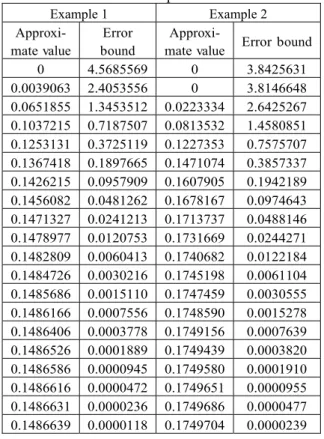
Table 1. Approximate value and error bound for Examples Example 1 Example 2 Approxi-mate value Error bound
Approxi-mate value Error bound
0 4.5685569 0 3.8425631 0.0039063 2.4053556 0 3.8146648 0.0651855 1.3453512 0.0223334 2.6425267 0.1037215 0.7187507 0.0813532 1.4580851 0.1253131 0.3725119 0.1227353 0.7575707 0.1367418 0.1897665 0.1471074 0.3857337 0.1426215 0.0957909 0.1607905 0.1942189 0.1456082 0.0481262 0.1678167 0.0974643 0.1471327 0.0241213 0.1713737 0.0488146 0.1478977 0.0120753 0.1731669 0.0244271 0.1482809 0.0060413 0.1740682 0.0122184 0.1484726 0.0030216 0.1745198 0.0061104 0.1485686 0.0015110 0.1747459 0.0030555 0.1486166 0.0007556 0.1748590 0.0015278 0.1486406 0.0003778 0.1749156 0.0007639 0.1486526 0.0001889 0.1749439 0.0003820 0.1486586 0.0000945 0.1749580 0.0001910 0.1486616 0.0000472 0.1749651 0.0000955 0.1486631 0.0000236 0.1749686 0.0000477 0.1486639 0.0000118 0.1749704 0.0000239
Figure 1. The trending diagram of Example 1
Figure 2. The trending diagram of Example 2
Depending on the approximate values and error bounds in Table 1, trending diagrams were con-structed as represented in Figures 1 and 2 for Exam-ples 1 and 2, respectively. From these figures, we can easily observe how these continuous linear program-ming problems come to a convergent value.
5. CONCLUSION
In the literature, some classic contributions in-troduced the separated concept to investigate the con-tinuous linear programming problems. However, most of these researches focused on verifying the theoretical result of optimal solution. In this study, we concerned with how the approximate optimal value and optimal solution of simple continuous lin-ear programming problems (SP) can be easily ob-tained. First using a discretization method we obtain finite dimensional linear programming problems (Pn)
from (SP). Then a recurrence method is provided for solving the dual problem of (Pn) and we also verify
that its optimal value is just to the approximate opti-mal value of (SP). Moreover, the optiopti-mal solution of (Pn) can be derived by the complementary slackness
theorem. Based on the optimal solution of (Pn), we
can easily construct an approximate optimal solution of the simple continuous linear programming prob-lem (SP).
ACKNOWLEDGEMENT
This research is supported under the grants of NSC 97-2115-M-037-001, NSC 97-2410-H-238-004 and NSC 97-2115-M-238-001, Taiwan, the Republic of China.
REFERENCES
1. Anderson, E. J., A Continuous Model for Job-shop Scheduling, PhD thesis, University of Cambridge, Cambridge, U.K. (1978).
2. Anderson, E. J., “A new continuous model for job-shop scheduling,” International Journal of Sys-tems Science, 12, 1469-1475 (1981).
3. Anderson, E. J. and P. Nash, Linear Programming in Infinite Dimensional Spaces, John Wiley and Sons, NY (1987).
4. Anderson, E. J. and A. B. Philpott, “A continuous time network simplex algorithm,” Networks, 19, 395-425 (1989).
5. Anderson, E. J. and A. B. Philpott, “Erratum a con-tinuous time network simplex algorithm,” Networks,
19, 823-827 (1989).
6. Anderson, E. J. and M. C. Pullan, “Purification for separated continuous linear programs,” Mathematical Methods of Operations Research, 43, 9-33 (1996).
7. Bellman, R., “Bottleneck problems and dynamic pro-gramming,” Proceedings of the National Academy of Sciences of the United States of America, Sep. 1, California, USA, 39, 947-951 (1953).
8. Bellman, R., Dynamic Programming, Princeton Uni-versity Press, Princeton, NJ (1957).
9. Buie, R. N. and J. Abrham, “Numerical solutions to continuous linear programming problems,” Mathe-matical Methods of Operations Research, 17, 107-117 (1973).
10. Drews, W. P., “A simplex-like algorithm for continu-ous-time linear optimal control problems,” in R. W. Cottle and J. Krarup (eds), Optimization Methods for Resource Allocation, Crane Russak & Co, NY, 309-322 (1974).
11. Fleischer, L. and J. Sethuraman, “Efficient algorithm for separated continuous linear programs: the multi-commodity flow problem with holding costs and extensions,” Mathematics of Operations Research, 30, 916-938 (2005).
12. Grinold, R. C., “Continuous programming part one: linear objectives,” Journal of Mathematical Analysis and Applications, 28, 32-51 (1969).
13. Grinold, R. C., “Symmetry duality for a class of con-tinuous linear programming problems,” Solving Scien-tific Problems with Mathematical Methods, 18, 84-97 (1970).
14. Hartberger, R. J., “Representation extended to con-tinuous time,” In R. W. Cottle and J. Krarup (eds), Optimization Methods for Resource Allocation, Crane Russak & Co, NY, 297-307 (1974).
15. Ho, T. Y., Y. Y. Lur and S. Y. Wu, “The difference between finite dimensional linear programming prob-lems and infinite dimensional linear programming problems,” Journal of Mathematical Analysis and Ap-plications, 207, 192-205 (1997).
16. Lehman, R. S., On the Continuous Simplex Method, Rand Corp Santa Monica, CA (1954).
17. Levinson, N., “A class of continuous linear program-ming problems,” Journal of Mathematical Analysis and Applications, 16, 73-83 (1966).
18. Pullan, M. C., “An algorithm for a class of continuous linear programs,” SIAM Journal on Control and Op-timization, 31, 1558-1577 (1993).
19. Pullan, M. C., “Forms of optimal solutions for sepa-rated continuous linear programs,” SIAM Journal on Control and Optimization, 33, 1952-1977 (1995). 20. Pullan, M. C., “A duality theory for separated
con-tinuous linear programs,” SIAM Journal on Control and Optimization, 34, 931-965 (1996).
21. Pullan, M. C., “Existence and duality theory for sepa-rated continuous linear programs,” Mathematical Modeling of Systems, 3, 219-245 (1997).
22. Pullan, M. C., “Convergence of a general class of algorithms for separated continuous linear programs,” SIAM Journal on Optimization, 10, 722-731 (2000). 23. Pullan, M. C., “An extended algorithm for separated
continuous linear programs,” Mathematical Pro-gramming, series A, 93, 415-451 (2002).
24. Segers, R. G., “A generalized function setting for dynamic optimal control problems,” In R. W. Cottle and J. Krarup (eds), Optimization Methods for Re-source Allocation, Crane Russak & Co, NY, 279-296 (1974).
25. Tyndall, W. F., “A duality theorem for a class of con-tinuous linear programming problems,” SIAM Journal on Applied Mathematics, 13, 644-666 (1965).
26. Tyndall, W. F., “A extended duality theory for con-tinuous linear programming problems,” SIAM Journal on Applied Mathematics, 15, 1294-1298 (1967). 27. Wang, X., Theory and Algorithms for Separated
Con-tinuous Linear Programming and Its Extensions, PhD thesis, The Chinese University of Hong Kong, Hong Kong, China (2005), in Chinese.
ABOUT THE AUTHORS
Ching-Feng Wen is currently an assistant professor in General Education Center at Kaohsiung Medical University, Taiwan. He received his M.S. in Depart-ment of Mathematics from the National Kaohsiung Normal University, Taiwan and the Ph.D. degree in Department of Mathematics from National Cheng
Kung University, Taiwan. His present research inter-ests include linear programming, fractional pro-gramming and infinite-dimensional optimization. Yan-Kuen Wu is a professor in the Department of Industrial Management at Vanung University, Tai-wan. He received his M.S. degree in Industrial Man-agement from the National Cheng Kung University, Tainan, Taiwan, in 1984 and the Ph.D. degree in In-dustrial Engineering from the Yuan Ze University, Taoyuan, Taiwan, in 1997. His research interests include fuzzy optimization and its applications, and mathematical programming.
Yung-Yih Lur is a professor in the Department of Industrial Management at Vanung University, Tai-wan. He received his Ph.D. degree in Department of Mathematics from Chung Yuan Christian University, Taiwan, in 1999. His research interests include fuzzy matrices and its applications, and mathematical pro-gramming.
(Received September 2008; revised November 2008; accepted November 2008)