以投球語意單元為基底的棒球影片結構分析與階層式摘要

全文

(1)國立交通大學資訊科學系碩士論文. 以投球語意單元為基底的棒球影片結構分析與摘要 Pitching Semantic Unit Based Baseball Video Structure Analysis and Summarization. 研究生：石永靖指導教授：薛元澤. 教授. 中華民國九十三年六月. i.

(2) 以投球語意單元為基底的棒球影片結構分析與階層式摘要 Pitching Semantic Unit Based Baseball Video Structure analysis and Summarization. 研究生：石永靖. Student：Yung-Ching Shih. 指導教授：薛元澤. Advisor：Dr. Yuang-Cheh Hsueh. 國立交通大學資訊科學研究所碩士論文. A Thesis Submitted to Institute of Computer and Information Science College of Electrical Engineering and Computer Science National Chiao Tung University in partial Fulfillment of the Requirements for the Degree of Master in Computer and Information Science June 2004 Hsinchu, Taiwan, Republic of China. 中華民國九十三年六月. ii.

(3) 以投球語意單元為基底的棒球影片結構分析與摘要. 學生：石永靖. 指導教授：薛元澤. 國立交通大學資訊科學學系﹙研究所﹚碩士班. 摘要. 在本篇論文中，我們提出一簡單的架構，僅使用少數的場景特徵如顏色及動量特徵有效率地分析 MPEG-2 棒球影片。我們的目標是偵測出大部分的重要事件並提供多階層式摘要。首先偵測投球場景，並將影片切割成一連串以投球場景為始的片段(投球語意單元，PSU)。接著利用主客場球衣顏色不同的特性，分析投手球衣顏色資訊找出換場事件(攻方、守方交替事件)，將影片半局為單位結構化。另外分析投球語意單元特徵，選出較長，較動態，要與球場上事件相關的內容當作重要事件。最後我們為每個選出的重要事件算分數以達成多層次摘要架構。在影片分析之後，我們能夠提供棒球影片的索引及多層次摘要內容，幫助使用者快速了解影片內容及增加影片的應用。實驗結果證實，我們方法是簡單有效的。. iii.

(4) Pitching Semantic Unit Based Baseball Video Structure Analysis and Summarization. student：Yung-Ching Shih. Advisors：Dr.Yuang-cheh Hsueh. Institute of Computer and Information Science National Chiao Tung University. ABSTRACT. In this thesis, we propose a simple framework only using a few cinematic features, such as color features and motion features to analyze the MPEG-2 baseball video efficiently. Our objective is to detect most of the highlight events, and supply multi-level summaries. We first detect the pitching shots, and divide the baseball video into a sequence of segments starting with a pitching shot (Pitching Semantic Units, PSU). Then we use the property of different uniform colors between home team and visit team to find out the change events (an exchange of offensive and defensive). Moreover, we analyze the PSU information to take events that are longer, more active, and more relevant to in-filed content as the highlight events. Finally, we compute a score for each highlight event to implement the multi-level summarization framework. After the analysis process, we can provide the indices and the multi-level summaries of the baseball video to help user to comprehend the video content quickly and extend the applications of the video. Experimental results indicate that the proposed method is simple and effective.. iv.

(5) 誌謝我在此要感謝我的指導教授薛元澤教授，兩年來對我悉心的指導與照顧，教導我研究學問的方法及待人處世的道理使我受益良多。同時也要感謝口試委員張隆紋教授及莊仁輝教授給予我的建議與指教，使論文內容更加完善。還要感謝詹森仁學長、楊朝棟學長、林瑞盛學長及林柏青學長他們給我論文研究及寫作方面的種種建議。感謝王聖博同學，廖偉智同學，江育寬同學，莊逢軒學弟，何昌憲學弟，王蕙綾學妹，高薇婷學妹陪伴我度過快樂的研究所生活。特別感謝智慧型系統實驗室李威德學長及林哲寬同學的協助，提供我相關的知識及程式碼，給予我實驗及程式實作上的許多幫忙。也非常感謝王承舜學長，洪啟倫同學，及李柏賢學弟的影片收集與提供。最後，我要感謝我最親愛的家人，我的父母親及姊姊，長久以來一直給予我關懷、支持與鼓勵。僅將本篇論文獻給我的家人，及所有幫助過我的人，謝謝你們，祝福你們永遠健康快樂。. v.

(6) CONTENTS ABSTRACT(CHINESE) ....................................................................................................iii ABSTRACT(ENGLISH) ....................................................................................................iv ACKNOWLEDGEMENT...................................................................................................v CONTENTS ...........................................................................................................................vi LIST OF FIGURES ............................................................................................................viii LIST OF TABLES .................................................................................................................x. Chapter 1 Introduction................................................................................................................1 1.1 Motivation ....................................................................................................................1 1.2 Sports Video Analysis Methods....................................................................................2 1.3 Organization of This Thesis..........................................................................................4 Chapter 2 Background Knowledge.............................................................................................5 2.1 Color models ................................................................................................................5 2.2 Overview of MPEG-2 Standard ...................................................................................7 2.3 Shot Change Detection Method..................................................................................12 2.4 Overview of MPEG-7 Multimedia Description Schemes ..........................................14 Chapter 3 The Proposed Method ..............................................................................................17 3.1 The Field Dominant Color Detection Method............................................................17 3.2 Shot Classification and Pitching Shot Detection........................................................22 3.2.1 Shot Classification...........................................................................................22 3.2.2 Pitching Shot Detection...................................................................................27 3.3 Event Detection and Summarization ..........................................................................29 3.3.1 Change Event Detection ..................................................................................30 3.3.2 Highlight Event Detection ...............................................................................32 3.3.3 Multi-level Summarization..............................................................................34 vi.

(7) Chapter 4 Experimental Results ...............................................................................................36 4.1 Experimental Environment and Test Data..................................................................36 4.2 Experimental Results..................................................................................................38 Chapter 5 Conclusions and Future Works ................................................................................45 References ................................................................................................................................47. vii.

(8) LIST OF FIGURES Fig. 1.1Multi-level FSU structures of a tennis program.............................................3. Fig. 2.1 The RGB Color Model..................................................................................6 Fig. 2. 2 The HSI Color Model...................................................................................7 Fig. 2. 3 The MPEG-2 video stream structure............................................................8 Fig. 2. 4 The GOP structure........................................................................................9 Fig. 2.5 (a) Motion compensation example for a FMB or a BMB (b) Motion compensation example for a BIMB.................................................................. 11 Fig. 2.6 Flow chart of spatial domain process..........................................................12 Fig. 2.7 Abrupt and gradual shot change chart .........................................................13 Fig. 2.8 The overview of the MPEG-7 Multimedia Description Scheme…………..15. Fig. 3.1 Two different fields and their HSI dominant color histograms...................19 Fig. 3.3 Rough Dominant Color Ranges ..................................................................21 Fig. 3.4 Histogram Analysis Chart ...........................................................................22 Fig. 3.5 Flow between Frames .................................................................................24 Fig. 3.6 (a) static state shot (b) replay shot (c) flow magnitudes of (a) (d) flow magnitudes of (b) .....................................................................................................25 Fig. 3.7. Pitching Frames and Three Corresponding Rectangles. ..........................28. Fig. 3.8 Pitching Semantic Units..............................................................................29 Fig. 3.9 (a) PAR in a pitching frame (b) PR in a pitching frame..............................30 Fig. 3.10 Pitcher block color analysis flow chart .....................................................31 Fig. 3.11 Examples of PSU events ...........................................................................33 Fig. 3.12 Time interval of PSU.................................................................................33 Fig. 3.13 Multi-level summaries of the baseball video ............................................35 viii.

(9) Fig. 4.1 The test baseball videos...............................................................................37 Fig. 4.2 Comparison of original data size and summarization data size ..................40 Fig. 4.3 Video1 Experimental Results ......................................................................41 Fig. 4.4 Video2 Experimental Results ......................................................................41 Fig. 4.5 Video3 Experimental Results ......................................................................42 Fig. 4.6 Video4 Experimental Results ......................................................................42 Fig. 4.7 Video5 Experimental Results ......................................................................43 Fig. 4.8 Video6 Experimental Results ......................................................................43 Fig. 4.9 An example of refining summarization process..........................................44. ix.

(10) LIST OF TABLES Table 4. 1 The information of the test videos ...........................................................37 Table 4.2 The Results of change event detection .....................................................38 Table 4.3 The Results of highlight event detection ..................................................40. x.

(11) Chapter 1 Introduction. 1.1 Motivation With the constantly growth in the amount of digital videos, more and more video data are available for users, and the demand of effective management for multimedia data is more and more significant. Some research areas such as video content analysis, the feature extraction, and the semantic level information understanding promote the effective management and specific applications for videos. MPEG-7 [1] has a goal to create a standard containing a comprehensive set of tools for describing the multimedia content data. It, however, does not standardize approaches for multimedia content description. The sports video is one of the most popular videos, and appears to a large audience. The value of the sports video and the audience’s interest, however, drop significantly after a period of time [2]. In many cases, users prefer to watch a sports video with a compact content (summary) containing most of the interesting segments of the original sports video. Sports video summaries are metadata of the original data and help users to efficiently comprehend the original content. Sports video summaries also increase the usage of the sports video such as delivering sports video over the narrow band networks, and the application in mobile devices with small storage. There are a number of researches about the sports video analysis. Superimposed caption texts are used to recognize some high level semantic information, such as score, ball count, and inning in the baseball video [5] [6]. Some researches about the specified baseball video contents classification and detection are proposed [7]-[11]. These approaches [7]-[11] use the statistical based learning methods to train the specific models for the predefined video contents, and then they use the models to classify and detect the video content. These 1.

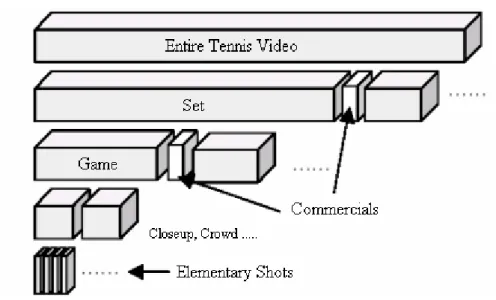
(12) approaches, however, need to extract a large number of multimedia features for each frame and shot, and compute the statistic results for models building, content classification and detection. These processes involve computationally extensive operations. In this thesis, we provide a simple framework for baseball video structure analysis and summarization. We only use a few cinematic features, such as color ratios and motion characteristics to analyze the baseball video content efficiently. After the analysis, we choose highlight events and create the multi-level summaries of the baseball video. In our method, we do not focus on classifying video content into detailed categories, instead we concentrate on detecting most of the important events in which audiences are interested and creating the summaries that greatly condense the baseball video.. 1.2 Sports Video Analysis Methods Sports videos are different from other videos such as news and dramas in the temporal structure and domain characteristics. In a sports video, a fixed number of cameras are set in specified positions of the field to take the particular views. The particular views occur periodically in the sports videos. Therefore, sports videos have regular temporal structures in content and many characteristics corresponding to games and fields. Change et al. [3] [4] proposed a method to analyze the temporal structure of the sports video by detecting the specific recurrent events. They [4] defined three related but distinct terms: views, fundamental semantic units (FSUs), and events to present the content structure in sports video. A view is the specific angle and the direction of a camera in a specific location of field. A shot is a continuous sequence of frames which is captured from a single camera during a time period [16]. Hence, there may be several views in a single shot. A FSU is defined as a recurrent video content unit. FSUs can be divided into multiple levels corresponding to important semantic activities. A FSU may consist of many views, and a video can be divided into a sequence of FSUs. Events are defined as the action occurrence in 2.

(13) the video, such as hit, serve, and score. A FSU contains a number of events. Fig. 1.1 [4] gives an example of multi-level FSU structures of a tennis program.. Fig. 1.1 Multi-level FSU structures of a tennis program A. Ekin et al. [2] proposed an automatic and computationally efficient framework for soccer video analysis and summarization using cinematic and object-based features. They first detect a single dominant color (a tone of green) of the soccer field. The shot boundaries are determined with the differences of grass color ratios of adjacent frames. The shot classification is accomplished with the frame grass color ratios and certain criteria. They also use measurement of frame difference to detect slow-motion replay. After the cinematic feature analysis, they define a cinematic template to detect the goal events. Furthermore, they detect the object-based features, such as the occurrence of the referees, and the penalty box with the distinguishable colored uniforms of the referees and the parallel lines in the field. Finally, they can provide the summaries of the soccer videos. As mentioned above, we understand that sports videos have the regular temporal structures, and we can use cinematic features to detect the specific video segments. In our method, we will utilize the specific temporal structures and cinematic features to analyze the baseball video and to detect the highlight events. In a baseball video, most events start with a pitching shot. Thus, we firstly detect the pitching shots. In the pitching shot detection process,. 3.

(14) we take the domain characteristics such as the field color ratio, the field color layout, the object layout, and the motion characteristics as the pitching shot characteristics, and the color features and the motion features from the video are extracted to match the pitching shot characteristics for the pitching shot detecting. After detecting the pitching shots, we divide the baseball video into a sequence of segments starting with a pitching shot. We call these segments as pitching semantic units (PSUs). The set of all PSUs in the baseball video contains almost total events in the baseball video. The important event is always the actively in-field content, and lengthens the interval between the current pitching shot and the next pitching shot. Thus, we consider that more important events are more active and relevant to in-field events in longer PSUs. We detect highlight events from PSUs according to the lengths, motion features, and color features in them. In addition, we compute a score for each highlight event and provide a multi-level summarization framework. In chapter 3, we will discuss our method in detail.. 1.3 Organization of This Thesis The remainder of this thesis is organized as follows. In chap 2, we will state the background knowledge, including the color spaces, MPEG-2 standard, shot change detection methods, and MPEG-7 multimedia description schemes. In chap 3, we will discuss our proposed baseball video analysis and summarization procedure, including the field dominant color detection, shot classification, pitching shot detection, PSU segmentation, change event detection, highlight event detection, and multi-level summarization. In chap 4, we will describe the implementation of our experiments in detail, and present the experimental results. In chap 5, we will state conclusions and future works.. 4.

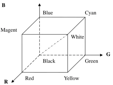
(15) Chapter 2 Background Knowledge. In this chapter we will introduce the background knowledge of our research. In section 2.1, we will describe the color models. In section 2.2, the MPEG-2 bitstream structure is stated. In section 2.3, the shot change detection methods are described. In section 2.4, we will introduce the MPEG-7 multimedia description schemes.. 2.1 Color models Color is a powerful descriptor that facilitates object identification and extraction. The purpose of a color model is to facilitate the specification of colors in some standard [12]. Most of the color models in use now are apply to hardware or some special applications. In this section, we will introduce the RGB, YCbCr, and HSI color models.. RGB Color Model: The RGB color model could be represented in a three-dimensional coordinate system. A color is associated with a three-dimensional vector of (R, G, B). The RGB color model is the most commonly used hardware oriented model, but it is not nature for human visual perception. The RGB color model is shown in Fig. 2.1.. 5.

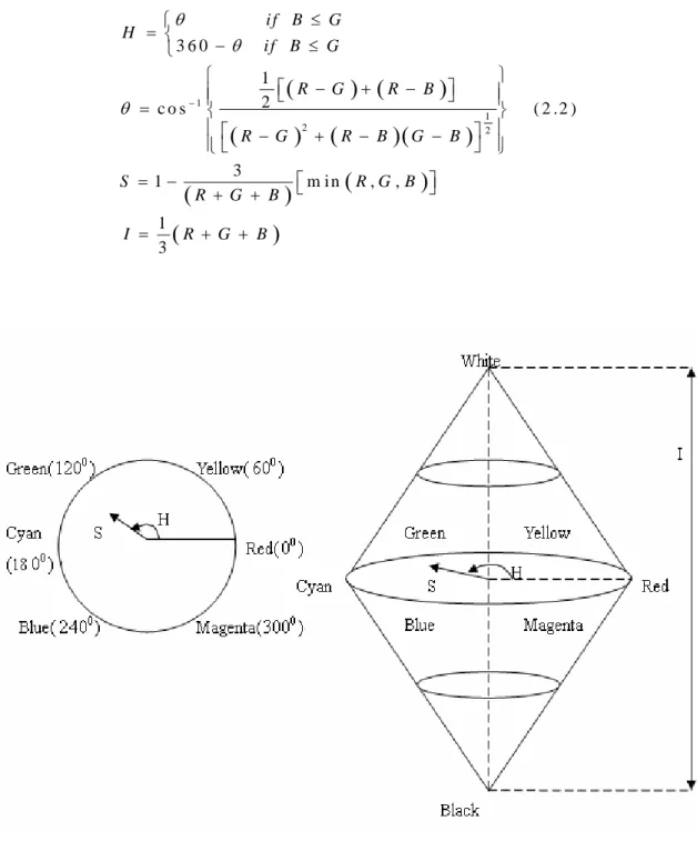
(16) B. Blue. Cyan. Magent White G. Black. R. Red. Green Yellow. Fig. 2.1 The RGB Color Model YCbCr Color Model: The YCbCr color model separates the luminance Y and two chromaticity values Cb, Cr from the color. Taking advantage of this property, the luminance and chromaticity can be coded in different number of bits. It is useful in image compression and widely used in JPEG and MPEG. The conversion of RGB to YCbCr is given as Eq. 2.1 [13].. Y = 0.299 R + 0.587G + 0.114 B Cb = −0.169 R − 0.331G + 0.500 B Cr = 0.500 R − 0.419G − 0.0813B. (2.1). HSI Color Model:. The HSI color model is formed with Hue, Saturation, and Intensity. Hue is used to describe a pure color. Saturation shows the degree of the dilution of pure color. Intensity is the brightness of the color. This model decouples the luminance and chromaticity, and is nature for human visual perception. Therefore, it has the advantages in some applications. In this paper, the video color features that we extract are based on the HSI color model. The HSI color model and the conversion functions from RGB are shown as follows.. 6.

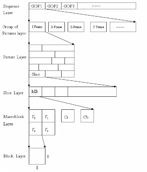
(17) ⎧θ H = ⎨ ⎩360 − θ. if B ≤ G if B ≤ G. ⎧ 1 ⎡ ( R − G ) + ( R − B ) ⎦⎤ ⎪ ⎪ 2 ⎣ θ = c o s −1 ⎨ 1 ⎪⎡ R − G 2 + R − B G − B ⎤2 ( ) ( )( ) ⎪⎩ ⎣ ⎦ 3 ⎡ m in ( R , G , B ) ⎤⎦ S =1− (R + G + B ) ⎣ I =. 1 (R + G + B 3. ⎫ ⎪⎪ ⎬ ⎪ ⎪⎭. ( 2 .2 ). ). Fig. 2. 2 The HSI Color Model. 2.2 Overview of MPEG-2 Standard MPEG-2 [14], an ISO/IEC standard which is proposed by Moving Picture Experts Group (MPEG) in order to support applications of future digital TV and the high quality video compression. In our experiments, all of the test videos are MPEG-2 format. The standard MPEG-2 video stream contains six layers: sequence, group of picture (GOP), picture, slice, 7.

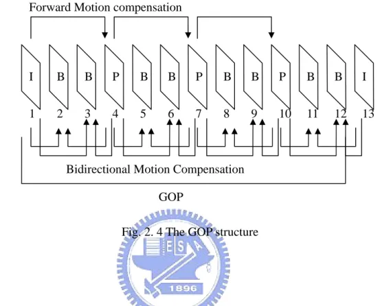
(18) macroblock (MB), and block. Fig. 2.3 [17] illustrates the MPEG video stream structure.. Fig. 2.3 The MPEG-2 video stream structure Sequence:. The sequence layer is the highest syntactic structure of the coded bitstream. It holds some parameters that are used in the decode process. Group of pictures (GOP):. The GOP provides the random access point. It consists of several frames, including three 8.

(19) types of frames (pictures), I frame (Intra-coded frame), P frame (Predictive-coded frame), and (Bidirectionally predictive-coded frame).. Fig. 2. 4 shows the structure of the GOP.. Forward Motion compensation. I. B. B. P. B. B. P. B. B. P. B. B. I. 1. 2. 3. 4. 5. 6. 7. 8. 9. 10. 11. 12. 13. Bidirectional Motion Compensation GOP Fig. 2. 4 The GOP structure. Picture:. MPEG defines three types of pictures (frames), I frame (Intra-coded frame), P frame (Predictive-coded frame), and B frame (Bidirectionally predictive-coded frame). They use different coding methods. Each type of frames consists of three components, a luminance component (Y), and two chrominance components (Cb, Cr). During the encoding and the decoding process, I frames use only the information itself, and they are also used as reference for P frames and B frames. P frames are coded using forward motion estimation and motion compensation from the previous I frame or P frame, and they serve as reference for P frames and B frames. B frames are coded using forward and backward motion compensation from previous and future reference frames. They do not serve as reference. Slice layer:. A slice avoids the bitstream error propagation influencing the whole frame. It is a series of macroblocks. All the macroblocks of a slice shall be in the same horizontal row. 9.

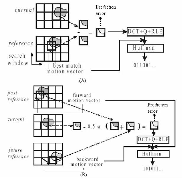
(20) Macroblock (MB) layer:. MB is the basic unit used for motion estimation and compensation. MB is a 16*16 size region in the frame. It consists of a section of luminance component and the spatially corresponding chrominance components. There are four types of MB in MPEG-2. IMB (intra-coded MB) can be coded by itself. FMB (forward-prediction MB), BMB (backward-prediction MB), and BIMB (bidirectionally-prediction MB) perform forward reference, backward reference, and bidirectionally reference respectively. I frames contain only IMBs. P frames contain IMBs and FMBs. B frames contain IMBs, FMBs, BMBs, and BIMBs. Block layer:. A block is a set of 8*8 pixels and is a basic unit used in DCT transform.. Inter-Coding:. Inter-coding is done through motion compensation process. During the encoding process each MB of P and B frame is tested to compare the costs of motion compensation and intra-coding, and the one which is more economic will be chosen. During the motion compensation process, the encoder finds the best matching region in the reference frame(s) and calculates the prediction error and one or two motion vectors (MVs) for each MB of current frame. Fig. 2.5 [15] illustrates the motion compensation examples.. 10.

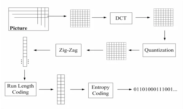
(21) Fig. 2.5 (a) Motion compensation example for a FMB or a BMB(b) Motion compensation example for a BIMB. Spatial domain compression:. During the Spatial domain compression process, blocks of the frame are inputted into DCT transform, then the quantization, Zig-Zag scan transform, run length coding and entropy coding are performed. The flow chat is shown in the Fig. 2.6. Blocks in IMB contain the original information, and blocks in FMB, BMB, and BIMB contain the prediction errors of motion compensation.. 11.

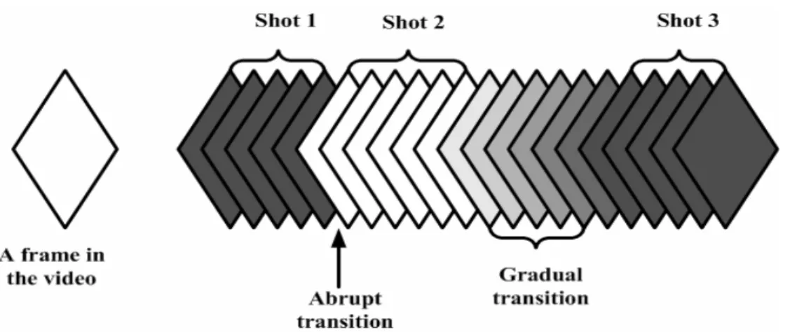
(22) Fig. 2.6 Flow chart of spatial domain process. 2.3 Shot Change Detection Method A shot is defined as a continuous sequence of frames which is captured from a single camera during a time period [16]. It could be represented as an event or a subject. The shot change detection is the first step of video processing. In some applications, such as video retrieval and indexing, a shot is a basic unit of a video segment. A shot change is a transition between two adjacent shots. There are two main types of shot changes: abrupt type and gradual type. The abrupt type is that the transition from one shot to another is a single frame, and the gradual type is that shot changes occur across multiple frames with some video editing skills making the transition look smooth. Fig. 2.7 illustrates the two types of transitions.. 12.

(23) Fig. 2.7 Abrupt and gradual shot change chart. The shot change detection is to detect the shot change locations by comparing the difference of adjacent frames. Some shot change detection methods are proposed such as the pixel based method, the histogram based method, the feature based method, the DCT coefficient based method, the DC image based method, and the MB based method. These approaches can be roughly distinguished into uncompressed domain and compressed domain methods. The former is used for raw data, and the latter is used for compressed data such as MPEG. In the following paragraphs, we will briefly discuss these methods. Uncompressed domain:. The pixel based method detects the shot change by the pair-wise pixel comparison of frames. It is good for content variation but is too sensitive to noise and computation costly. The histogram based method compares the histograms of adjacent frames. This method is more robust to noise but lacks the pixel spatial information affecting the accuracy. The feature based method extracts the edge features of the corresponding frames. It is good for obtaining the shape characteristics but is computation costly and too sensitive to noise. Compressed domain:. The DCT coefficient based method uses the I frame DCT coefficients to detect the shot change positions. This method is computation efficient. However, it only utilizes I frames that will result in missing the precise shot change positions. The DC image is a thumbnail 13.

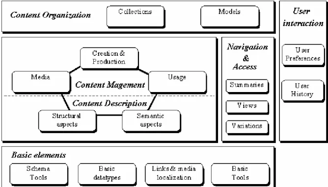
(24) consisting of DC values of the original MPEG frame. The DC image based method compares the adjacent DC images to find the shot change locations. This method is efficient and robust to noise. The MB based methods [20] use the MB information to find the shot change positions out. This type of methods is simple and fast, but the MB information may differ with different encoders. Lee [17] proposed a compressed domain shot change detection method on the MPEG. He firstly used the computationally efficient MB information to select the shot change candidate frames. In the second phase, only the DC images of the selected candidate frames are extracted to further detect the precise shot changes. Thus, the computation is efficient in his method, and the two-phase detection process makes the more precise detection results. In this thesis, our test baseball videos have been preprocessed with the shot change detection using the program provided by Lee [17].. 2.4 Overview of MPEG-7 Multimedia Description Schemes MPEG-7 [1] is an ISO/IEC standard proposed by Moving Picture Experts Group (MPEG), and has a formal name “Multimedia Content Description Interface”. MPEG-7 will not replace other MPEG standards such as, MPEG-1, MPEG-2 and MPEG-4, since it is intended to provide a comprehensive set of tools for describing the multimedia content instead of the content itself. However, MPEG-7 does not standardize approaches for multimedia content description. The objective of MPEG-7 is only to standardize the interfaces (descriptors) between the client application and the search engine [22]. MPEG-7 defines Multimedia Description Schemes (MDS) that combine low-level, and high-level features to describe the multimedia content. Fig.2.8 [1] illustrates an overview of the organization of MPEG-7 MDS which consists of six components: Basic Elements, Content Description, Content management, Content Organization, Navigation and Access, and User Interaction. 14.

(25) Fig. 2.8 The overview of the MPEG-7 Multimedia Description Scheme. (1)Basic Elements:. These description schemes (DSs) provide specific data-type and mathematical structures, and address specific needs for multimedia data descripiton such as time position, persons, individuals, groups, organization, and textual annotation. (2)Content Management:. These DSs describe the creation information, usage information and media description. (3)Content Description:. The content description elements describle the structure (regions, video frames, audio segments) and semantic (objects, events, abstract annotation) of the multimedia data. In the structural aspect, multimedia data is described in the viewpoint of content structure. In the conceptual aspect, the multimedia is described in the view point of real-world semantics and conceptual notions. (4) Navigation and Access:. These DSs provide the facilitating browsing and retrieval of multimedia content by defining the summaries, decompositions, and variations of the multimedia content. There are 15.

(26) two types of summaries DSs, hierarchical mode and sequential mode. Hierarchical mode summaries have multiple levels. The levels close to root provide coarser summaries, and the higher levels provide the more detail summaries. Sequential mode summaries provide a sequences of video frames, possibly synchronized with audio, which may compose of a slide-show or audio-visual skim [1]. (5)Content Organization:. The content organization DSs organize the collection of multimedia content segments, and describe their common properties. They can group multimedia contents into clusters and describe the relation of among clusters. (6) User Interaction:. These DSs deal with user information, such as personal preferences and user histories.. 16.

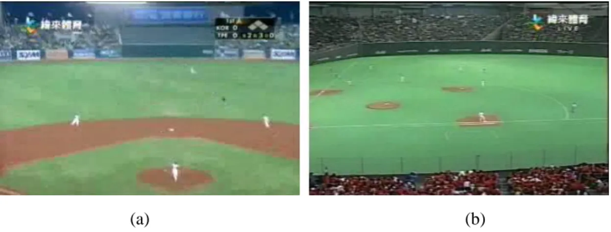
(27) Chapter 3 The Proposed Method In this chapter, we discuss our baseball video analysis and summarization scheme in derail. In section 3.1, we describe the field dominant color detection method. In section 3.2, we use motion features and color features to classify shots into some categories and detect the pitching shots. In section 3.3, we retrieve the pitching semantic units (PSUs), then detect the changes events and the highlight events, and provide the multi-level baseball video summaries.. 3.1 The Field Dominant Color Detection Method There are two dominant colors in a baseball field: grass and sand colors. They are very useful when using in shot classification and identification. However they differ from stadium to stadium. Thus, the dominant color ranges of baseball fields are different. Fig. 3.1 shows two different baseball fields and corresponding HSI histograms. The charts in the left column belong to (a), and the others belong to (b). It reveals that the dominant colors of these two fields are notable different. Thus, we cannot set a specific value for the color of the field.. (a). (b). Fig. 3.1 Two different fields and their HSI dominant color histograms (continued) 17.

(28) Fig. 3.1 Two different fields and their HSI dominant color histograms (continued). 18.

(29) Fig. 3.1 Two different fields and their HSI dominant color histograms. In [3], Zhong et al. built a tennis court dominant color information database that contains enough games so that the color information of a new game will be similar to one in the 19.

(30) database. In [2], A. Ekin et al assume the existence of a single dominant color (a tone of grass) that indicates the soccer field, and detect this dominant color range by analyzing the HSI color histograms. In our method, we suppose that baseball fields contain two dominant colors, and we use the histogram analysis method to detect the color ranges. Fig. 3.2 displays the flow chart of the field dominant color detection process. First, two predefined rough field dominant color ranges, RGS (a tone of grass with hue 60 ∼ 180 and saturation > 0.06 ), and RSD (a tone of sand with hue 0 ∼ 60 and saturation > 0.06 ) are used to choose appropriate frames for further analysis. The precise field dominant color ranges are the subsets of the rough ranges. Fig. 3.3 shows two rough field dominant color ranges. Second, we choose the appropriate frames containing enough field dominant color ratios for further analysis later. The choosing rules specified in Eq. 3.1-3.3 eliminating the inappropriate frames, like close-up, spectators, lounge and so on. Because the regions of grass and sand are always presented in the bottom of the frame, RatioRGS is defined as the ratio of RGS in the bottom half frame, and RatioRSD is the ratio of RSD in the bottom half frame. TRGS , TRSD , and TRGS + RSD are corresponding thresholds in the rules.. Rough color ranges HSI histograms analysis Frames choosing Precise color ranges. Fig. 3.2 Flow chart of field dominant color detection. 20.

(31) Fig. 3.3 Rough Dominant Color Ranges. RatioRGS > TRGS. (3.1). RatioRSD > TRSD. (3.2). RatioRGS + RatioRSD < TRGS + RSD. (3.3). Finally, we analyze the histograms of the choosing frames to get the precise field dominant color ranges. We compute two sets of histograms from the choosing frames. One is about the grass color, where the grass color information comes from the pixels in RGS. The other is about the sand color, where the sand color information comes from the pixels in RSD. Each set of histograms contains three components Hue, Saturation, and Intensity. Then we analyze each histogram according to Eq. 3.4-3.9 [2], where H refers to the histogram, i peak is the peak index of each histogram, [imin , imax ] is the determined range of the histogram, K is a value between 0 and 1 used to adjust imin and imax . Fig. 3.4 illustrates the concept of the histogram analysis. After analyzing six histogram ranges we obtain two precise dominant color ranges, the grass color range (GS), and the sand color range (SD).. 21.

(32) Fig. 3.4 Histogram Analysis Chart. H [imin ] ≥ K * H [i peak ]. (3.4). H [imin − 1] < K * H [i peak ]. (3.5). H [imax ] ≥ K * H [i peak ]. (3.6). H [imax +1 ] < K * H [i peak ]. (3.7). imin ≤ i peak. (3.8). imax ≥ i peak. (3.9). 3.2 Shot Classification and Pitching Shot Detection In this section, we first classify shots into some categories according to the motion features and color features. The shot classification results will be used to detect the pitching shots and highlight events in the following analysis processes.. 3.2.1 Shot Classification Motion energy:. Zhang et al. [21] proposed a concept of motion energy for video frames to display the motion activities of frames. The video frames are divided into a number of blocks. The motion energy of the nth frame is the summation of the displacements of the total blocks from the (n − 1)th frame to the nth frame. In a baseball video, each shot may contain. 22.

(33) different content variations and different number of frames. We compute motion energy of each shot in a baseball video to estimate shot motion activities, and classify them into categories according to their motion energy. We do not compute motion information from consecutive frames with computationally expensive operations, instead, we directly use the motion vectors (MVs) information of P frames to efficiently approximate the motion energy. In Eq. 3.10, we define the motion energy of a frame, ME ( f ) , as the summation of total motion vector lengths of the frame, where. MVv 2 (i, j ) + MVh 2 (i, j ) is the length of. (i, j )th motion vector MV (i, j ) with vertical and horizontal components MVv (i, j ) and MVh (i, j ) respectively. In Eq. 3.11, the motion energy of a shot ME ( Shot ) is defined as the mean value of total motion energy of P frames in this shot, where pf k is the kth P frame in the shot, and tf is the number of total P frames in the shot. After obtaining the motion energy, then we classify shots into specified categories. Eq.3.12 presents that a shot belongs to S (small motion energy shot), M (median motion energy shot), or L (large motion energy shot) according to the magnitude of motion energy, where Tme _ low and Tme _ med are the corresponding thresholds. m. n. ME ( f ) = ∑∑ MVv 2 (i, j ) + MVh 2 (i, j ). (3.10). i =1 j =1 tf. ME ( Shot ) =. ∑ ME ( pf k =1. k. ) (3.11). tf. ⎧ Shot ∈ S if ME ( Shot ) < Tme _ low ⎪ ⎨ Shot ∈ M if Tme _ low ≤ ME ( Shot ) < Tme _ med ⎪ ⎩ Shot ∈ L if Tme _ med ≤ ME ( Shot ). (3.12). Flow magnitude between frames:. In [18], V. Kobla et al. proposed a concept of flow of frames to display the motion relation of adjacent frames in the video. They use the forward-predicted motion vectors and 23.

(34) backward predicted motion vectors of B frames in a Sub-GOP structure to derive the flow vectors of each frame in the Sub-GOP structure. Fig. 3.5 represents the flows between the frames in a SGOP structure, where Ri and R j are two reference frames, each of which may be an I frame or a P frame. The flow of the kth frame flowk in the video can be thought as the collection of its flow vectors. The flow magnitude of a frame is defined as the summation of its total flow vector lengths. The flow direction relating to video play sequence is always in backward, so we are more interested in flow magnitude.. Fig. 3.5 Flow between Frames. Through the flow magnitude information, we can estimate the motion activities of the corresponding successive frames. If flow magnitudes of frames are large, the content of corresponding frames is active. On the contrary, if flow magnitudes of frames are small, the content of corresponding frames is static. If a number of successive flow magnitudes are very small in a shot, then we can suppose that the shot contains static states or still frames. Some still frames caused by video editing usually appear with a replay. Fig. 3.6(a) presents a static state (motionless content) in a shot, and Fig. 3.6 (c) is the corresponding flow magnitude chart. Fig. 3.6 (b) shows a replay, and Fig. 3.6 (d) is the corresponding flow magnitude chart. In Fig. 3.6 (c), and (d), we can see that a number of successive flow magnitudes which are very small, and we name this phenomenon SFMS (Successive Flow Magnitudes are Small).. 24.

(35) Fig. 3.6 (a) static state shot (b) replay shot (c) flow magnitudes of (a) (d) flow magnitudes of (b) 25.

(36) We classify the shots that contain SFMS phenomenon as R (containing static states or replay characteristics) type shots. Eq.3.13 defines a rule to detect SFMS, where Mag ( flowk ) is the flow magnitude of the kth frame, and fm _ s is a small flow magnitude threshold and n is a successive frames number threshold. In Eq.3.14, if a shot contains SFMS then it belongs to R type.. ⎧cont (i, n) = 1 if ∀ Mag ( flowk ) < fm _ s, ( k = i to i + n − 1) ⎨ ⎩cont (i, n) = 0 else. (3.13). , cont (l − n − 1, n)) = 1 ⎧Union(cont (1, n), cont (2, n), shot ∈ R if ⎨ (3.14) ⎩l = number of total frames of the shot. Grass color ratio:. If the grass color ratio of a shot is high, then we suppose that this shot is more relevant to in-field events. On the other hand, if the ratio is low, then we suppose that this shot is irrelevant to in-field events. Therefore, we compute the grass color ratio of shots and classify them into Gs (small grass color ratio) type and Gl (large grass color ratio) type. Eq.3.15 indicates computation of the grass ratio of a shot, gs ( shot ) , where gs ( f k ) means the grass color ratio of the frame f k , and the frames f k , f k + g ,. , f k + g * t are the sampling frames. included in the corresponding shot. In Eq.3.18, a shot is classified into Gs or Gl by shot grass ratio threshold Tgs .. gs ( shot ) = max( gs ( f k ) , gs ( f k + g *1 ) , , fk , f k + g ,. , gs ( f k + g * t ) ). , f k + g * t ∈ shot. ⎧⎪ shot ∈ Gs if gs( shot ) < Tgs ⎨ ⎪⎩ shot ∈ Gl if gs( shot ) ≥ Tgs. (3.15). (3.16). 26.

(37) 3.2.2 Pitching Shot Detection. The pitching shot is a very important shot in a baseball video. Most events in the baseball video start with a pitching shot. There are many regular domain characteristics of pitching shots in the baseball video, such as the fixed camera view, the field color layout, the frame object layout, and the small motion activities. Fig. 3.7(a) illustrates a pitching shot. A pitcher is on the left side of the frame, and a batter, a catcher and an umpire are on the right side of the pitcher. The bottom half frame contains specific field color layout (two clusters of sand) and dominant color ratios. Because of the fixed camera view and less camera motions, the motion energy of this shot is very small. In most baseball videos, pitching shots are presented in very similar ways. Thus we use these stable and constant domain characteristics to detect the pitching shot. Our pitching shot detection method is based on the pitching frame detection. If a pitching frame is found and the motion rule is satisfied, then a pitching shot is detected. In the pitching shot detection process, we use the color features and motion features to match the domain characteristics. We first detect the main objects, such as the pitcher, the batter, the catcher and the umpire. We just need to know whether the frame has objects in the corresponding position, thus we do not need the extract the precise object shapes with expensive computation cost. We fully used the domain knowledge in the pitching shot to set two rectangle regions, rt1 and. rt2 in appropriate positions. We use color ratios in rt1 and rt2 to recognize whether objects are in the corresponding regions. Fig. 3.7 (b) and (c) illustrate rt1 , and rt2 respectively. Afterward we set another rectangle region, rt3 , to detect the specific field characteristics, such as field dominant color layout and color ratios. The region rt3 is shown in Fig. 3.7 (d).. 27.

(38) Fig. 3.7 Pitching Frames and Three Corresponding Rectangles.. Eq. 3.17-20 are pitching frame detection rules. Ratio _ rt1 and Ratio _ rt2 are ratios of non-grass color and non-sand color in rt1 and rt2 respectively. Ratiogs _ rt3 and. Ratiosd _ rt3 are the ratios of grass color and sand color in rt3 respectively. In Eq. 3.20 Sand _ cluster is the number of sand clusters in rt3 . There are two clusters of sand in the pitching frame, one is the batter region and the other is the pitcher hill. If Eq. 3.17-20 are all satisfied, then a pitching frame is detected. After a pitching frame is detected, finally the motion information will be checked to detect the pitching shot. Eq. 3.21 is the motion rule. It means that the pitching shot belongs to S type, or the pitching shot belongs to M type and motion energy of the detected pitching frame is small. If Eq. 3.17-21 are all satisfied, then the pitching shot is detected.. 28.

(39) Tlow _ rt1 < Ratio _ rt1 < Thigh _ rt1. (3.17). Tlow _ rt 2 < Ratio _ rt2 < Thigh _ rt 2. (3.18). ⎧ Ratiogs _ rt3 > Tgs _ rt 3 ⎪ ⎨ Ratiosd _ rt3 > Tsd _ rt 3 ⎪ ⎩ Ratiogs _ rt3 + Ratiosd _ rt3 < Tgsgd _ rt 3. (3.19). Sand _ cluster = 2. (3.20). ⎧(i ) ⎪ ⎨or ⎪(ii ) ⎩. (3.21). Shot ∈ S Shot ∈ M. and ME ( f p ) ≤ Tme _ low. 3.3 Event Detection and Summarization In the baseball video, pitching shots appear periodically. Most events in a baseball video start with a pitcher shot. Thus, we divide baseball video into a series of segments starting with a pitching shot called pitching semantic units (PSUs). In the following sub-sections, we will detect change events and highlight events from PSUs and provide the hierarchical summaries. Fig. 3.8 illustrates the PSU structure in a baseball video.. Fig. 3.8 Pitching Semantic Units 29.

(40) 3.3.1 Change Event Detection. A change event is an exchange of offensive and defensive, and it is also the boundary of two successive half innings. Change events structurally divide a baseball game into several segments (half innings). In most formal baseball games, home team and visit team have different uniform colors. We distinguish the two uniform colors, and identify the pitcher uniform change among the PSUs to detect the change events. The purpose of the change event detection is to avoid erroneous recognition of highlight events and to structure the baseball video content. In a pitching shot, we know the approximate position of the pitcher. However, we do not know the precise region of pitcher to analyze pitcher’s uniform color. We set a pitcher approximate rectangle region (PAR) containing most part of the pitcher in the approximate position. Then we search a suitable pitcher rectangle region (PR) closely containing the pitcher’s uniform in PAR by filtering out the regions containing more grass color and sand color ratios from left to right, and from bottom to top. Fig. 3.9 (a) and (b) illustrate the PAR and PR respectively.. (a). (b). Fig. 3.9 (a) PAR in a pitching frame (b) PR in a pitching frame. After the PR has been found, we analyze the color information in the PR. Fig. 3.10 shows the analysis flow chart. First, we filter out the grass color and sand color regions in PR. 30.

(41) Second, we divide the remaining part into to gray part and color part with saturation value, and get the gray pixels ratio value ( R1 ). Finally, we analyze histograms to get the corresponding i peak , imin , and imax (Eq. 3.4-3.9), and to compute gray part intensity ( R2 ), color part hue value ( R3 ), and color part intensity value ( R4 ) according to Eq. 3.22.. Fig. 3.10 Pitcher block color analysis flow chart. value = i peak * peak _ weight + imin * min_ weight + imax * max_ weight. (3.22). For each PSU, R1 , R2 , R3 , and R4 are acquired to represent the pitcher uniform color information, and we cluster all PSUs into two groups according to these representative values. The clustering method that we use is McQueen’s k-means method [19]. In Eq.3.23-3.26, Cn is the centroid of the nth group, Cn _ R1 , Cn _ R2 , Cn _ R3 , and Cn _ R4 are representative values of Cn , Pk is the kth PSU pitcher uniform color. information, Pk _ R1 , Pk _ R2 ,. Pk _ R3 , and Pk _ R4 are its representative values. Eq.3.27 defines the distance of one. 31.

(42) extracted color information of the mth PSU Pm to the centroid of the nth group Cn where α i the corresponding weights. After the clustering process, we search the cluster change positions PSU by PSU along the temporal playing sequence to find PSUs contain the change events. Cn _ R1 = Cn _ R2 = Cn _ R3 = Cn _ R4 =. ∑ (P _ R ) k. 1. Cn. ∑ (P _ R ) k. 2. Cn. ∑ (P _ R ) 3. k. Cn. ∑ (P _ R ) k. 4. Cn. distance(Cn , Pm ) =. ∑ ( (C 4. i =1. n. , ∀ Pk ∈ Cn. (3.23). , ∀ Pk ∈ Cn. (3.24). , ∀ Pk ∈ Cn. (3.25). , ∀ Pk ∈ Cn. (3.26). _ Ri − Pm _ Ri ) 2 * α i. ). (3.27). 3.3.2 Highlight Event Detection. After detecting the change events, we search the highlight events from the remainder PSUs. The highlight events in which we are interested are advantageous to offensive, such as hits, bunts, stealing bases, scores, sacrifice flies and defensive errors, or are meaning events such as pause events, dead balls and game ending events. These events may occur in a single PSU simultaneously. PSUs containing highlight events are longer and consist of more shots. Fig. 3.11 gives an example, PSU i contains a hit event and a score event, and consists of more shots than PSU j and PSU j +1 that have no important events. Therefore we choose highlight event candidates from longer PSUs. Eq.3.28-3.29 indicate the choosing rules, SN ( PSU k ) is the number of shots in PSU k , and Ti ( PSU k ) , is the total playing time of all shots of PSU k except the starting pitching shot. Fig. 3.12 illustrates the concept of Ti ( PSU ) . 32.

(43) SN ( PSU k ) > shot _ threshold. (3.28). Ti ( PSU k ) > time _ threshold. (3.29). Fig. 3.11 Examples of PSU events. Fig. 3.12 Time interval of PSU. 33.

(44) In addition, there is a phenomenon that highlight events contain active contents and in-field contents. After obtaining candidate PSUs, we filter out some inappropriate PSUs which are more static and are not relevant to in-field events. The filtering rules are listed below. 1. The starting pitching shot is adjacent with a S shot (small motion energy shot). 2. Too many S shots in the PSU (the number S shots is larger than the number of M shots and L shots). 3. The starting pitching shot is adjacent with a Gs shot (less grass color ratio shot).. Finally, we shorten the detected PSUs to present the highlight events appropriately. In most cases, using a whole PSU to present an event is too redundant, and the last few shots of PSU are meaningless. Thus, we want to provide a video segment containing appropriate length to represent a highlight event by finding a new end shot and cut off the later shots in the PSU. The rule is that an event retains at least first few shots in the PSU, and the new end shot is the first S shot or R shot in the later shots.. 3.3.3 Multi-level Summarization. In this subsection, we provide summaries of the baseball video. We propose a multi-level hierarchical framework to select the contents of the summaries. We can collect all the detected highlight events as the most detailed summary, or we can reduce highlight events to condense the summarization content. There is a trend that more important events are in the longer PSUs. In Eq. 3.30, the computation of the score of eventi , Score(eventi ) , is specified, where PSU c is the corresponding PSU of eventi , and Wt and Ws are adjustable weight parameters. Thus we compute score of each highlight event according to Eq. 3.30. Events in the longer PSUs obtain higher score. After computing the score for each detected event, we can provide the multi-level summarization with different number of highlight events. The multi-level summarization framework conforms to the concept of MPEG-7 34.

(45) hierarchical summary DSs. Fig. 3.13 illustrates the concept of the multi-level summarization. Higher levels provide more detailed summaries, and lower levels only containing higher score events provide coarser summaries. Users can choose the suitable summary according to their needs. Score(eventi ) = Ti ( PSU c ) *Wt + SN ( PSU c ) *Ws. (3.30). Fig. 3.13 Multi-level summaries of the baseball video. 35.

(46) Chapter 4 Experimental Results In this chapter, we present the experimental results of baseball video analysis and summarization. In section 4.1, we state the experimental environments and the test baseball video data. In section 4.2, we discuss the experimental results.. 4.1 Experimental Environment and Test Data Our experimental environment is Microsoft Windows XP Professional operating system on an IBM compatible PC with an Intel P4 2.0 GHz CPU and 256 megabytes RAM. The program was developed in the C language and compiled under Microsoft Visual C++ 6.0. The utilized MPEG2 decoder is the open source developed by Berkeley Multimedia Research Center. We verify our method by making experiments on six test cases, two of them are Taiwan baseball videos, two of them are Japan baseball videos, and the others are American baseball videos. The total length of the videos is about 16 hours. These baseball videos include 5 different stadiums from 3 different channels. All of these videos are of the MPEG-2 format with the 352*240 resolution at 30 fps. Table 4.1 and Fig. 4.1 indicate the information of 6 test videos. All of the baseball videos were shot change detected using the method and program proposed by Lee [17]. Because of the gradual shot changes always occur in the relaxing moments and replays, gradual shot change detection may divide the non-highlight event PSU into more shots and influences the precision of the highlight event detection. Thus, in the shot change detection, we only focus on the abrupt type. In our experiments, the preprocessing time is about 37 minutes, and the analysis time is about 43 minutes for one hour length videos in average. 36.

(47) Video. Game. Frames. Length. Video1 2001 Baseball World Cup Game55. 237844. 2:12:08. Video2 2001 Baseball World Cup Game64. 274962. 2:32:55. Video3 2003 Asian Baseball Championship Game4. 286915. 2:39:23. Video4 2003 NPB Nippon series Game1. 337255. 3:07:22. Video5 2001 MLB World Series Game3. 311001. 2:52:47. Video6 2001 MLB World Series Game4. 257438. 2:23:08. Table 4. 1 The information of the test videos. Fig. 4.1 The test baseball videos. 37.

(48) 4.2 Experimental Results We use the Precision and Recall measure to evaluate the performance of experimental results. Precision and Recall are indicated in Eq.4.1 and 4.2, where C is the number of correct detected relevant events, F is the number of false detected events, C+F is the number of total detected events, M is the number of missed relevant events, and C+M is the number of total relevant events.. Precision = Recall =. C C+F. (4.1). C C+M. (4.2). Table 4.2 shows the result of change events detection. In most cases, the results are satisfied. The results in Video4 are worse than other videos, because the luminance of rear part is instable. Three of the false detected events in Video4 are in the neighbor of the positions of three missed change events. Although these false detected events cannot show the precise change event positions, they also structure the game with intervals of half innings.. Video. Correct. Miss. False. Precision. Recall. Video 1. 16. 0. 2. 88.89%. 100%. Video 2. 17. 0. 0. 100%. 100%. Video 3. 15. 1. 1. 93.75%. 93.75%. Video 4. 14. 3. 4. 77.78. 82.35%. Video 5. 15. 1. 0. 100%. 93.75%. Video 6. 17. 1. 2. 89.4%. 94.4%. Table 4.2 The Results of change event detection Table 4.3 presents the results of highlight events detection. The highlight events in which we are interested are advantageous to offensive such as hits, bunts, stealing bases, scores, 38.

(49) sacrifice flies, and defensive errors, or are meaning events such as pause events, dead balls, and game ending events. The precisions and recalls of the highlight event detection are computed by comparing the detected results and the human observation results. The average precision of all test videos is about 53%, and the average recall of all test videos is about 86% in our experiments. Some false detected highlight events which do not belong to defined highlight events are still meaningful, such as walks, infield outs, outfield outs, and base progressive events. These events also provide useful information about the game to the audiences. Fig. 4.2 illustrates the comparison of the original data sizes and the summary sizes of highlight events in our experiments. The summary data sizes are about 7%-13% of the original data sizes, and the lengths of the summaries are about 12~24 minutes. After detecting the highlight events and providing the most detailed summary, we can also condense the summary progressively to provide multi-level summaries. We compute a score for each detected highlight event according to Eq.3.30. Then we reserve the higher score events and filter out the lower score events. The number of reserve events is according to the reserve ratio. The reserve ratio is defined in Eq.4.3, where RE is the number of reserve events, and TH is the number of total detected highlight events. Fig. 4.3-4.8 present precisions, recalls, and time ratios of the re-condensed results in Video1-Video6. We can discover that as the highlight event reserve ratio decreases, the precision increases, and the recall and time ratio decreases. In other worlds, the re-condensed summary has higher precision and the coarser content. It is a tradeoff between precision and recall. Some applications like delivering sport video over narrow band networks, using mobile device to browse video, and quickly realizing the game result need the short summary content with high precision, thus the refining summarization process is a feasible solution.. Reserve Ratio =. RE TH. 39. (4.3).

(50) Video. Correct. Miss. False. Precision. Recall. Video 1. 20. 2. 16. 55.55%. 90.91%. Video 2. 21. 1. 12. 63.63%. 95.45%. Video 3. 25. 5. 21. 54.34%. 83.33%. Video 4. 24. 2. 27. 47.06%. 92.31%. Video 5. 16. 5. 14. 53.33%. 76.19%. Video 6. 14. 4. 15. 48.27%. 77.77%. Table 4.3 The Results of highlight event detection. Original Size Summary size. Seconds. 11245. 12000 10000. 9175. 9563. 10366 8588. 7928. 8000 6000 4000 2000. 934. 958. 667. 1426. 1015. 844. 0 Video 1. Video 2. Video 3. Video 4. Video 5. Video 6. Fig. 4.2 Comparison of original data size and summarization data size. 40.

(51) Precision. Precision. 100%. 100%. 80%. 80%. 60%. 60%. 40%. 40%. 20%. 20%. 0%. 0% 100% 90%. 100% 90% 80% 70% 60% 50% 40% Reserve Ratio. 80%. 70%. 60%. 50%. 40%. Reserve Ratio. 4.3(a) Video1 precision of re-condensed summaries. 4.4(a) Video2 precision of re-condensed summaries. Recall. Recall 100%. 100% 80%. 80%. 60%. 60%. 40%. 40%. 20%. 20%. 0%. 0%. 100% 90% 80% 70% 60% 50% 40%. 100%. 85%. Reserve Ratio. 70% 55% Reserve Ratio. 40%. 4.4(b) Video2 Recall of re-condensed summaries. 4.3(b) Video1 Recall of re-condensed summaries Time Ratio. Time Ratio. 14.0%. 8%. 12.0%. 7%. 10.0%. 6%. 8.0%. 5% 4%. 6.0%. 3%. 4.0%. 2%. 2.0%. 1% 0%. 0.0%. 100%. 100% 90% 80% 70% 60% 50% 40% Reserve Ratio. 90%. 80%. 70% 60% Reserve Ratio. 50%. 40%. 4.3(c) Video1 Time Ratio of re-condensed summaries. 4.4(c) Video2 Time Ratio of re-condensed summaries. Fig. 4.3 Video1 Experimental Results. Fig. 4.4 Video2 Experimental Results. 41.

(52) Precision. Precision. 100.00%. 100%. 80.00%. 80%. 60.00%. 60%. 40.00%. 40%. 20.00%. 20%. 0.00%. 0% 100%. 85%. 70% 55% Reserve Ratio. 40%. 100% 90% 80% 70% 60% 50% 40% Reserve Ratio. 4.6(a) Video4 precision of re-condensed summaries. 4.5(a) Video3 precision of re-condensed summaries. Recall. Recall 100.00%. 100%. 80.00%. 80%. 60.00%. 60%. 40.00%. 40%. 20.00%. 20%. 0.00%. 0%. 100% 90% 80% 70% 60% 50% 40% Reserve Ratio. 100% 90% 80% 70% 60% 50% 40% Reserve Ratio. 4.5(b) Video3 Recall of re-condensed summaries. 4.6(b) Video4 Recall of re-condensed summaries. Time Ratio. Time Ratio. 14%. 12%. 12%. 10%. 10%. 8%. 8%. 6%. 6%. 4%. 4%. 2%. 2% 0%. 0% 100% 90% 80% 70% 60% Reserve Ratio. 100% 90% 80% 70% 60% 50% 40% Reserve Ratio. 50% 40%. 4.5(c) Video3 Time Ratio of re-condensed summaries. 4.6(c) Video4 Time Ratio of re-condensed summaries. Fig. 4.5 Video3 Experimental Results. Fig. 4.6 Video4 Experimental Results. 42.

(53) Precison. Precision 100%. 100%. 80%. 80%. 60%. 60%. 40%. 40%. 20%. 20% 0%. 0% 100% 90%. 80%. 70%. 60%. 50%. 100% 90% 80% 70% 60% 50% 40% 30%. 40%. Reserve Ratio. Reserve Ratio. 4.7(a) Video5 precision of re-condensed summaries. 4.8(a) Video6 precision of re-condensed summaries. Recall. Recall. 100%. 100%. 80%. 80%. 60%. 60%. 40%. 40%. 20%. 20%. 0%. 0% 100% 90%. 80%. 70% 60% Reserve Ratio. 50%. 40%. 100% 90% 80% 70% 60% 50% 40% 30% Reserve Ratio. 4.7(b) Video 5 Recall of re-condensed summaries. 4.8(b) Video 6 Recall of re-condensed summaries. Time Ratio. Time Ratio. 12%. 12%. 10%. 10%. 8%. 8%. 6%. 6%. 4%. 4%. 2%. 2%. 0%. 0%. 100% 90%. 80% 70% 60% Reserve Ratio. 50%. 100% 90% 80% 70% 60% 50% 40% 30% Reserve Ratio. 40%. 4.7(c) Video 5 Time Ratio of re-condensed summaries. 4.8(c) Video 6 Time Ratio of re-condensed summaries. Fig. 4.7 Video5 Experimental Results. Fig. 4.8 Video6 Experimental Results. 43.

(54) After analyzing the baseball video, we can provide indices for it. There are three types of indices, pitching shots, highlight events, and half innings (according the change events). Moreover, we can provide multi-level summaries according to the number of the reserve events. Fig. 4.9 gives a re-condensed summarization example of Video5. The total length of Video5 is 172 minutes 46 seconds. The most detailed summary contains all detected 30 events with precision of 53%, and the length is 16 minutes 55seconds with time ratio of 9%. After a re-condensed summarization process, we reserve the top 35% highlight events according to the corresponding scores. This re-condensed summary contains 10 events with precision of 70%, and its length is 6 minutes 39 seconds with time ratio of 3%.. Fig. 4.9 An example of refining summarization process. 44.

(55) Chapter 5 Conclusions and Future Works In this thesis, we proposed a pitching semantic unit (PSU) based baseball video structure analysis and hierarchical summarization method. We efficiently use the color features, and motion features to detect the pitching shots and to classify shot types. After detecting the pitching shots, we segment the baseball video into a sequence of PSUs. We detect change events and highlight events from the PSUs and compute a score for each highlight event to accomplish providing the multi-level summaries. Characteristics of our proposed method include the following. 1. We propose a simple framework and only use fewer features to analyze the baseball videos efficiently. 2. We provide three types of indices, pitching shots, detected highlight events, and half innings in the baseball video. 3. The multi-level summaries help users to comprehend a baseball game quickly, and users can choose their needed summary according to their preference. The higher level summaries provide more detailed contents, and the lower level summaries provide the coarser contents. 4. The summaries greatly condense the baseball video in time, and they will raise the usage of the baseball video such as delivering over narrow band network and application in mobile devices.. In our work, we focus on detecting most highlight events efficiently, but we do not further classify these events into some categories. In the future, people can extract more characteristics from the PSUs and integrate other features such as audios, textures, and 45.

(56) caption information in the video to classify the detected events into some categories, to get more high-level semantic information, and to promote the highlight event detection precision.. 46.

(57) References [1]. N. Day and J. M. Martinez, “Overview of the MPEG-7 Standard (version 4.0),” ISO/IEC JTC1/SC29/WG11 N4675 Jeju, March 2002. [2]. A. Ekin, A. M. Tekalp, and Rajiv Mehrotra “Automatic Soccer Video Analysis and Summarization,” IEEE Trans. Image Processing, Vol. 12, No. 7, pp. 796-807, July 2003. [3]. D. Zhong and S. F. Chang, “Structure Analysis of Sports Video Using Domain Models,” IEEE International Conference on Multimedia and Expo, pp. 22-25, August 2001. [4]. S. F. Chang, D. Zhong and R. Kumar, “Real-Time Content-Based Adaptive Streaming of Sports Videos,” Content-Based Access of Image and Video Libraries,. 2001 (CBAIVL 2001) IEEE Workshop on, Dec 2001 [5]. T. Kawashima, K. Tateyama, T. Iijima and Y. Aoki, “Indexing of Baseball Telecast for Content-based Video Retrieval,” IEEE International Conference on Image. Processing, vol.1, pp. 871-874, Oct 1998 [6]. D. Zhang and S. F. Chang, “Event Detection in Baseball Video Using Superimposed Caption Recognition,” 10th ACM International Conference on Multimedia, pp. 315-318, 2002. [7]. C. L. Huang and C. Y. Chang, “Video summarization using Hidden Markov Model,” IEEE International Conference on Information Technology: Coding and. Computing, pp. 473-477, 2001 [8]. H. C. Shih and C. L. Huang, “Image Analysis and Interpretation for Semantics Categorization in Baseball Video,” IEEE International Conference on Information. Technology: Coding and Computing [Computers and Communications], pp.. 47.

(58) 379-383, 2003 [9]. W. Hua, M. Han and Y. Gong, “Baseball Scene Classification Using Multimedia Features,” IEEE 2002. [10]. P. Chang, M. Han and Y. Gong, “Extract Highlights From Baseball Game Video with Hidden Markov Models” IEEE International Conference on Multimedia and. Expo, Vol. 1, pp. 821-824, Aug. 2002 [11]. M. Han, W. Hua, W. Xu and Y. Gong, “An integrated Baseball Digest System Using Maximum Entropy Method,” ACM international conference on Multimedia, pp. 347-350, 2002. [12]. R. C. Gonzales and R. E. Woods “Digital Image Processing,” Prentice Hall, 2002. [13]. D. S. Taubman, M. W. Marcellin, “JPEG2000: image compression fundamentals, standards, and practice,” Kluwer Academic Publishers, 2002. [14]. ISO/IEC IS 13818-2, MPEG-2 Video. [15]. F. Idris and S. Panchanathn, “Review of Image and Video Indexing Technique”,. Journal of Visual Communication and Image Representation, Vol. 8, No. 2, pp. 146-166 1997 [16]. I. Koprinska and S. Carrato, “Temporal Video Segmentation: A Survey,” Signal. Processing: Image Communication, Vol. 16, pp. 477-500, 2001 [17]. W. T. Lee, “MPEG Video Analysis – Shot Change Detection and Classification,” Master Thesis, Institute of Computer and Information Science, National Chaio Tung University, 2003. [18]. V. Kobla, D. Doermann, K. I. Lin, and C. Faloutsos, “Compressed domain video indexing techniques using DCT and Motion Vector information in MPEG video,” in. Proc. of the SPIE Conference on Storage and Retrieval for Still Image and Video Databases V, vol. 3022, pp200-211, 1997 [19]. J. B. McQueen, “Some methods of classification and analysis of multivariate 48.

(59) observations,” In Proc. of 5th Berkeley Symp. on Mathematical Statistics and. Probability, pp. 281-297, 1967 [20]. S.C. Pei and Y. Z. Chou, “Efficient MPEG Compressed Video Analysis Using the Macroblock Type Information,” IEEE Trans. Multimedia, Vol. 1 No. 4, PP. 321-333, 1999. [21]. X.D. Zhang, T. Y. Liu, K. T. Lo, and J. Feng, “Dynamic Selection and Effective Compression of Key Frames for video abstraction,” Pattern Recognition Letters, Vol. 24, pp. 1523-1532, 2003. [22]. Z. H. Liu, “A Content Retrieval System Based on MPEG-7 Descriptors and JPEG2000 for Mobile Applications,” Master Thesis, Institute of Computer and Information Science, National Chaio Tung University, 2003. 49.

(60)