行政院國家科學委員會專題研究計畫 成果報告
動態財務分析與模擬最佳化在產險公司的應用(2/2)
研究成果報告(完整版)
計 畫 類 別 : 個別型 計 畫 編 號 : NSC 95-2416-H-004-009- 執 行 期 間 : 95 年 07 月 01 日至 96 年 07 月 31 日 執 行 單 位 : 國立政治大學風險管理與保險學系 計 畫 主 持 人 : 蔡政憲 共 同 主 持 人 : 何憲章、陳春龍 計畫參與人員: 博士班研究生-兼任助理:黃孝慈、詹芳書、詹淑卿 碩士班研究生-兼任助理:劉婉玉、鄭嘉峰、林家樂 助理教授:游子宜 報 告 附 件 : 出席國際會議研究心得報告及發表論文 處 理 方 式 : 本計畫涉及專利或其他智慧財產權,2 年後可公開查詢中 華 民 國 96 年 11 月 01 日
行政院國家科學委員會補助專題研究計畫 成果報告
動態財務分析與模擬最佳化在產險公司的應用
計畫類別:個別型計畫
計畫編號:NSC 95-2416-H-004 -009
執行期間:
94 年 6 月 1 日 至 96 年 7 月 31 日
計畫主持人:蔡政憲
共同主持人:何憲章、陳春龍
計畫參與人員:游子宜、黃孝慈、詹芳書、詹淑卿、林家樂、鄭嘉峰、
劉婉玉
成果報告類型(依經費核定清單規定繳交):完整報告
執行單位:國立政治大學
中 華 民 國 96 年 10 月 31 日
中文摘要
資產配置對產險公司的營運很重要。資產配置會影響產險公司的收益、風險、財務 健全度、甚至保費的釐定。因此不論是產險公司的經理人、股東、監理機關、以及評等 公司都很注重產險公司的資產配置。 學術界提供了兩大類的資產配置方式:效率前緣分析以及動態控制法。前者是在單 期的架構下分析投資組合的期望報酬率與風險,忽略了其他的統計量,多期來看也通常 得不到最佳的結果。動態控制法在理論上無懈可擊,可是只能在極特殊的假設下才能求 出封閉解,數量方法也只能處理少數幾個狀態變數,因此在實務上幾乎沒有實用價值。 想跳脫效率前緣單期的架構,又不想落入動態控制執行困難窘境的業者,大多先以效率 前緣的方法先求出第一期的資產配置,然後隨著市場的變化,再定時或不定時地回歸第 一期的配置。此外,財務的文獻在討論資產配置時都沒有考慮到產險的業務,而保險的 文獻也沒有人討論到產險公司的最適資產配置。 本計畫利用近年來在作業研究領域有長足發展的模擬最佳化,求解產險公司可能的 最適資產配置。我們先開發產險公司的營運模擬程式。這類的程式在歐洲被稱為內部模 型,在美國則是用於動態財務分析。程式中產險公司可以投資於現金、各種到期時間的 公債、股票、以及不動產,其業務則有長尾與短尾兩大類,其損失發展期間各為十期與 三期。模擬的期間是26 期。寫好產險公司的模擬程式後,我們再以基因演算法以及演化 策略法,在國家高速電腦中心的電腦上,以平行處理的方式,藉著多次的模擬,找出可 能的最適資產配置。經過仔細的比較後,我們確定利用模擬最佳化所找出的解,比運用 效率前緣或回歸法的結果還好。因此,這個計畫的結果除了對保險文現有貢獻之外,還 有潛在的實用價值。 本計畫的結果至少可以產生三篇學術論文。第一篇已經投稿出去,第二篇即將完成, 第三篇也已經有完整的結果了。 關鍵詞:產險公司、資產配置、模擬最佳化Abstract
Asset allocation is imperative to property-casualty (P/C) insurance companies. It affects an insurer’s return, risk, solvency, and even premium setting. Various stakeholders including managers, shareholders, regulators, and rating agencies pay close attention to the asset allocation of the P/C insurer.
The literature provides two ways for asset allocation: efficient frontier analysis and dynamic control method. The former analyzes a portfolio’s return and standard deviation under a single-period framework. This method ignores other statistics of the outcomes and generates sub-optimal results in multiple periods. Dynamic control method is theoretically sound. However, closed-form solutions can be obtained under rare circumstances and numerous methods can handle only few state variables. Investors who want to execute multi-period asset allocation rely on the so-called re-balancing methods. This method has no theoretical justifications though. Furthermore, the finance literature does not take the
underwritten businesses into account. The insurance literature, to our knowledge, provides no reference for the optimal asset allocation of P/C insurers.
This project utilizes one of the recent advances in operational research, simulation optimization, to search the optimal asset allocation of a P/C insurer. We first develop a program to simulate the operations of the insurer. The simulated insurer can invest in cash, bonds with different maturities, stock, and real estate. The insurer underwrites both short- and long-tail businesses. The simulation goes on for 26 periods. Then we apply the genetic algorithms (GA) and evolution strategies (ES) upon the developed program to solve the optimization problems. We employ parallel computation to simulate sufficiently large number of simulations to secure the robustness of our optimization search. The resulted
allocations do perform better that the ones obtained using the efficient frontier and re-balancing methods. Our results thus have potential practical value in addition to the contribution to the insurance literature.
This project will results in at least three journal articles. We have submitted one paper to an international journal and are wrapping up the second one. The results for the third paper are in hands already.
報告內容
以下的內容分為三節。第一節是一篇由本計畫產生的審查中論文1。第二節則是由本
計畫產生的第二篇論文,剛完成初稿。第三節是打算用來寫第三篇論文的結果。
第一節
Combining Dynamic Financial Analysis with Simulation Optimization to
Solve the Asset Allocation Problem of the Property-Casualty Insurer
aTzu-Yi Yu b
Department of Information Management
National Chi Nan University, Nantou Hsien, Taiwan, R.O.C.
Chenghsien Tsai
Department of Risk Management and Insurance National Chengchi University, Taipei, Taiwan, R.O.C.
Chuen-Lung Chen
Department of Management Information System National Chengchi University, Taipei, Taiwan, R.O.C.
a The authors are grateful to Jia-Le Lin for his competent programming assistance, to National Center for
High-Performance Computing of Taiwan for using its facility, and to the National Science Council of Taiwan for its financial support (project number NSC 94-2416-H-004-041).
b Corresponding Author. No. 1, University Road, Puli, Nantou Hsien, Taiwan, 545, R.O.C.
ABSTRACT
Dynamic financial analysis (DFA) is a useful decision-support system for the insurer, but it lacks optimization capability. The contribution of this paper is that it incorporates a
simulation optimization technique into a DFA system. With the ability to optimize, the DFA system proposed in this paper was able to solve the asset allocation problem of a
property-casualty insurance company. The simulation optimization technique used herein is a generic algorithm, and the optimization problem is a constrained multi-period asset allocation problem. We find that coupling DFA with simulation optimization resulted in significant improvements over a basic search method. The result was robust across random number sets. Furthermore, the resulting asset allocation changes with the parameters of the risk models as well as the insurer’s specifications in a way that is consistent with the differences in the parameters. Incorporating optimization features in DFA is therefore feasible, useful, and robust and should create considerable interest in the insurance industry.
Keywords: dynamic financial analysis; simulation optimization; asset allocation JEL Classification: G22, C61
I. INTRODUCTION
How to manage a property-casualty (P&C) insurance company is a major issue for various stakeholders including managers, shareholders, policyholders, and regulators. More specifically, the concerns are as to how a number of factors such as asset allocation, trading styles, capital structure, business growth, business allocation, reinsurance arrangement, and other decisions affect the value and the solvency of a P&C company. Assessing these various decisions is difficult, however, because a P&C insurance company is subject to double-sided uncertainties: the liability risk as well as the asset risk. In addition to the uncertainty regarding asset values, P&C insurance companies do not know how much they will have to pay for the products they sold. A comprehensive tool that simultaneously assesses both the liability and the asset risks of a P&C insurer is essential to competent and sound management.
The dynamic financial analysis (DFA) system is promising. A company-wide DFA system can simulate the distribution of an insurer’s surplus/equity at some point of time in the future under various assumptions about the insurer’s underwriting and investment strategies, the underwriting outcome, and the evolution of the financial markets. An insurer’s value and risk/solvency can then be defined upon the simulated surplus distribution, and people can use the simulated surplus distribution to make choices among alternative strategies. More specifically, a DFA system is capable of incorporating an insurer’s new businesses, the uncertain payments for the insurance products sold, the insurer’s asset allocation/disposition decisions, and the stochastic returns of financial assets to dynamically simulate the evolution of the insurer’s financial conditions. Alternative underwriting and/or investment strategies can then be compared based on how they affect the development of the insurer’s financial
conditions. For instance, an insurer can use a DFA system to assess asset allocation strategies by examining the impacts of alternative strategies on the surplus distribution over a target time horizon. The DFA system therefore can help managers make investment and business
The DFA system has two major advantages over the commonly used financial ratio analysis and other static analyses. First, a DFA system can incorporate future external
changes and internal decisions in addition to the information embedded in financial ratios.2 It is therefore superior to static analyses for profiling an insurer’s financial strength. Second, a DFA system explicitly considers the relations among risk factors and financial variables. Risk factors such as interest rates, equity asset prices, and real estate prices are correlated. The values of an insurer’s various types of assets are thus correlated with each other as well. Financial variables are further bound by two simple equations:
t i j t j t i Liability Surplus Asset − =
∑
,∑
, , and (1) t i j t j t i Liability Surplus Asset − ∆ =∆ ∆∑
,∑
, (2), where Asseti,t and Liabilityj,t represent the values of individual asset and liability items at time
t respectively, and ∆(.) denotes the change of the variable. The first equation depicts the
fundamental relations among financial variables at any point in time; the second equation captures the dynamic relations among the variables across time. The financial ratio analysis and other static analyses have difficulties in taking full account of the correlations, fundamental relations, and dynamic relations among the variables.
The construction of a DFA system for the P&C insurance company dates back to almost two decades ago. Insurance and actuarial scholars started conceptual discussions in the late 80s (Pentikainen, 1988; Taylor and Buchanan, 1988; Coutts and Devitt, 1989; Paulson and Dixit, 1989; Taylor, 1991). The British Institute of Actuaries Working Party on Insurance Solvency and actuaries soon developed P&C insurance company simulation models that could be used to evaluate the solvency of a company (Daykin et al., 1989; Daykin and Hey, 1991; Daykin, Pentikainen, and Pesonen, 1994). The Casualty Actuarial Society of the United
2 The information embedded in financial ratios is taken into account in the DFA system in the form of the initial
States embarked upon a long-term, multi-stage project entitled “Dynamic Financial Analysis” in the mid 90s. Starting from identifying risk factors and variables, this project not only developed general specifications for insurance company financial models but also studied refined issues such as model parameterization, result interpretation, and management/strategic usage. The potential of a DFA model was demonstrated by Cummins, Grace, and Phillips (1999) in which the scenario analysis conducted using a simple cash flow model outperformed the early warning and capital requirement systems employed in the United States for the P&C insurance company.
The DFA system, albeit powerful, tells us only which proposed strategy is better. It cannot tell us what the optimal strategy is. The DFA system generates surplus distributions, given users’ input about initial positions and strategies. It does not have the
mechanism/algorithm to search for the optimum. Managers therefore have to make educated guesses on what the optimal strategy looks like and employ the trial-and-error method to shoot for a good strategy. Trying all possible strategies to seek for the optimum is infeasible due to the large number of decision variables. A DFA system without an optimization mechanism is therefore incapable of helping managers maximize the shareholders’ value. The goal of this paper is to illustrate how to couple the technique of simulation optimization with a DFA system so that an insurer can use the improved DFA system for making optimal decisions.
Simulation optimization is the process of determining the values of the controllable input variables that optimize the values of the stochastic output variables generated by a simulation model. The controllable input variables, also called decision variables, in the case of a DFA may include asset allocation, trading frequency, rebalancing interval, capital structure, business growth, business allocation, and reinsurance arrangement.3 The output variables, also called the response variables, are usually a function of the expected value of simulated
3 A simulation model might also have parameters that are not controllable. For instance, the financial market and
surplus, insolvency probability, and other concerns of the board (e.g., meeting the capital requirement). The simulation model itself (a DFA system in this paper) can be thought of as a complex function mapping controllable input values to response values.4 In short, the
simulation optimization problem can be characterized as a stochastic search over a feasible exploration region (Keys and Rees, 2004).5
Tekin and Sabuncuoglu (2004) classified the techniques for simulation optimization into two main headings: local optimization and global optimization. Local optimization techniques assume that response values have a uni-modal surface. Some of them are iterative while some require gradient information. Therefore, when the response surface is
high-dimensional, discontinuous, and/or non-differentiable, local optimization techniques are often trapped into a local optimum and fail to find the optimal solution. On the other hand, global optimization techniques such as evolutionary algorithms, simulated annealing, and tabu search can be applied to these types of problems, and they are designed for problems with multi-modal response surfaces.
The contribution of this paper is applying one of these global optimization techniques to a DFA system to solve the asset allocation problem of the property-casualty insurance company. Our DFA system contains four asset classes (cash, bonds, stocks, and real estate) and two types of insurance businesses (long- and short-tail businesses) to capture the essence of the insurance company’s operations. Although the DFA system is simple when compared with commercial packages, it is complex enough to preclude one from finding optimal decision
4 Due to its stochastic nature, repeated runs of the model lead to different outputs even when using the same
values of controllable inputs. The average value of the output is often calculated, and the deviations from the average are subsequently analyzed.
5 The feasible region is defined by the practical limits on the ranges of the controllable inputs. Examples of
practical limits include short-sale constraints and upper bounds on portfolio weights faced by most financial institutions. The optimization problem is difficult to solve for several reasons. First, the function represented by the simulation model is almost always unknown. Second, the deviations from the average are usually significant, heterogeneous over the feasible region, and not normally distributed. Third, the feasible region is usually large because of the large number of controllable variables.
variables analytically.6 We therefore resort to some of the recent developments in simulation optimization. We choose one of the most popular evolutionary algorithms (EAs), the genetic algorithms (GAs), to optimize our DFA system. EAs work on a population of solutions in such a way that poor solutions become extinct while good solutions evolve to reach for the optimum. The most popular EAs are GAs, evolutionary programming (EP), and evolution strategies (ES). EP and ES have not yet been widely used in simulation optimization, but GAs have been successfully applied to the optimization problems arising in complex manufacturing systems (Tekin and Sabuncuoglu, 2004). In our simulation optimization problem, the objective function incorporates the expected discounted surplus as well as the insolvency probability. This objective function will result in an asset allocation that balances return with risk. The optimization problem is formulated as a multi-period one with
short-sale constraints.7
Our results show that the application of simulation optimization to DFA is feasible, useful, and robust. Our GA introduces a significant improvement over a basic search method. The resulting “optimal” asset allocations look reasonable without extreme positions.8
Furthermore, our method is robust across different random numbers. The value of the objective function is insensitive to the generated random numbers. Different parameter sets result in different optimal asset allocations, as expected, and the changes in the optimal solutions are comprehensible with respect to the differences in the parameters. Therefore it can be concluded that the application of simulation optimization in DFA is successful.
6 The impossibility is due to three reasons. First, the system contains several types of stochastic processes. The
function represented by the simulation model is thus unknown. Second, the variations of the outcomes generated by the system are significant, heterogeneous over the feasible region, and not normally distributed. Third, the system has 12 controllable variables over real intervals. The feasible region is therefore large.
7 Such a problem is difficult to solve. It can be attacked by the methods of dynamic programming, and the
solutions are characterized by the Hamilton-Jacobi-Bellman (HJB) partial differential equations. However, the HJB equation has only been solved in few specific cases. Even if the solution can be obtained, the required long-winded technicalities are awkward for practical uses. The short-sale constraints make the problem even more difficult.
8 Readers should be aware that simulation optimization is a heuristic search method. The existence of the
optimal solution is not proven, and there is no verification theorem to show that the resulted solution from simulation optimization is at least as good as all other solutions. The word “optimal” is used loosely in this paper to mean “the best known solution.”
The rest of this paper is organized as follows. Section 2 describes our DFA system, including the setting of the financial markets and insurance markets, the dynamics of the representative insurer’s financial positions, and the optimization problem of the insurer. In Section 3 our genetic algorithm is described in detail. It starts with an introduction to
simulation optimization and is followed by a brief review on genetic algorithms and a detailed description of our proposed algorithm. The application results are discussed in Section 4. We first provide the simulated interest rates, equity index, and real estate index to display some outputs of our DFA system. Then we demonstrate a basic searching method for the
single-period asset allocation problem and end section 4 with analyzing the results using our GA. Finally, in Section 5 we make our summaries and draw our conclusions.
II. THE DYNAMIC FINANCIAL ANALYSIS SYSTEM
A. The financial markets and the insurance markets
In this section, we set up five types of markets and specify their stochastic processes. We assume that the risk-neutral process for the one-year spot rate at time t, r(t), is:
( ) (
t q m r t)
dt r t dWdr = − ( ) +σKr ( ) K (3) , where t is zero or a positive integer, stands for the long-term average of spot rates, reflects the speed of mean reverting (
m q 1 0< q< ), σKr =[v 0 0 0 0], and ] [ ( ) ( ) ′ = dWr dWS dWRE dWLR L dWLR S W
d K . Wd K represent the differentials of
five-dimension Wiener processes including the processes of the one-year spot rate (r), the equity index (S), the real estate index (RE), the loss ratio of the long-tail insurance liabilities (LR(L)), and the loss ratio of the short-tail lines (LR(S)). It has a correlation matrix ℜ specifying the correlations among the Wiener processes. The mapping from short rates to Treasury bond prices has been derived in Cox, Ingersoll, and Ross (1985): the price at time t of a default-free zero-coupon bond that pays $1 at time T equals
r t T B T t r A T t e P ( ) 0( ) ) , ( = − − − (4)
, where T is a positive integer, T ≥t, γ 2 ) 1 )( ( ) 1 ( 2 ) ( + − + − = rxrx e q r e x B , 2 2 ) ( 2 0 2 ) 1 )( ( 2 ) ( σ γ γ γ γ qm rx q x e q e x A ⎥ ⎥ ⎥ ⎦ ⎤ ⎢ ⎢ ⎢ ⎣ ⎡ + − + = + , and γ = q2 +2v2 .
The equity index is assumed to evolve according to the following interest-rate-adjusted geometric Brownian motion process:
W d dt t r t S t dS S S K K σ π + + =( ( ) ) ) ( ) ( (5)
, where the constant parameter πS denotes the risk premium on the stock index investment, and σKS =[0 σS 0 0 0]. We assume that the real estate index follows a geometric Brownian motion: W d dt t RE t dRE RE K K σ µ + = ) ( ) ( (6)
, where the constant parameter µ denotes the expected return of the real estate investment per period with continuous compounding, and σKRE =[0 0 σRE 0 0].
In the insurance markets, insurers underwrite both long-tail and short-tail businesses. We assume that the loss ratio of the long-tail businesses follows:
W d t
L
dLR( )( )=σKLR(L)× K (7)
, where σKLR(L) =[0 0 0 σLR(L) 0]. The loss ratio of the short-tail lines has a similar process to equation (7) with a different volatility σKLR(S) =[0 0 0 0 σLR(S)].
The parameters for the above five models are specified as follows.
Model Parameters
Equity Index πS = 6% σS = 20%
Real Estate Index µ = 15% σRE = 35% Loss Ratio (Long) mean = 75% σLR(L) = 30%
Loss Ratio (Short) mean = 80% σLR(L) = 25%
The starting value of the short-term interest rate is 6%. Furthermore, the correlation matrix ℜ is specified as follows.9 dWS dWr dWLR(L) dWRE dWS 1 -0.31 -0.19 0.36 dWr -0.31 1 -0.004 -0.03 dWLR(L) -0.19 -0.004 1 -0.47 dWRE 0.36 -0.03 -0.47 1
B. The dynamics of the insurer’s financial status
Suppose that a newly established property-casualty insurer starts to underwrite insurance businesses with a surplus of IS(0) million dollars. It receives premiums of IP(0) million dollars in cash at the beginning of year 1 with B(0) (0≤ B(0)≤1) being the proportion of the businesses in the long-tail lines. To underwrite these businesses, the insurer incurs and pays underwriting expenses in cash and upfront. The underwriting expense ratios of the long- and short-tail businesses are assumed to be Exp(L) and Exp(S) respectively, where both ratios are positive but smaller than one.
The remaining cash and the initial surplus are then invested in cash, Treasury bonds, equity index, and real estate index with the proportion vector θK(0), where
9 The correlation coefficients are estimated using the historical data on S&P 500 index, Indexes of All Publicly
Traded REITs, Treasury Bill Rates, and the loss ratios published in Best’s Aggregates and Averages. The
sampling period is from 1972 to 1999. dWLR(S) is not in the matrix because we assume that the loss ratio of short-tail businesses is independent of other processes.
[
]
′= (0) (0) (0) (0) )
0
( θ1 θ2 θ3 θ4
θK , θ1(0), θ2(0), θ3(0), and θ4(0) is the proportion of the wealth invested in cash, equity index, Treasury bonds, and real estate index respectively. Obviously
∑
i4=1θi(t)=1. We further assume that θi(t)≥0 since insurers are almost always subject to short-sale constraints from regulation. The maturity of invested bonds ranges from one year to fifteen years, and the invested proportions are assumed to be even across the maturities for the sake of simplicity. Assuming that the fair value of the reserves equal to the premiums written net of expenses, we get the following balance sheet of the insurer at the beginning of year 1:
Assets Liabilities and Surplus
Cash $ (θ1(0)*Total Assets) Liabilities of
Long-Tail Businesses
$ B(0) * IP(0) * (1-Exp(L))
Stocks $ (θ2(0)*Total Assets) Liabilities of
Short-Tail Businesses $ (1- B(0)) * IP(0) * (1-Exp(S)) Treasury Bonds $ (θ3(0)*Total Assets)
Real Estate $ (θ4(0)*Total Assets) Surplus $ IS(0)
Total Assets
$ (IS(0)
+ B(0)*IP(0)*(1- Exp(L)) + (1-B(0))*IP(0)*(1-
Exp(S)))
Total Liabilities and Surplus
$ (IS(0)+ B(0) * IP(0) * (1- Exp(L)) + (1-B(0)) * IP(0) *
(1- Exp(S)))
stochastic models in section A.10 To account for loss development and business growth we assume that the insurer’s long-tail businesses grow G(L) annually and have a ten-year development period with a loss development function DL(dy), where dy = 1, 2, 3, …, or 10,
, and . The short-tail businesses have an annual growth rate of G(S) and a three-year development period with a loss development function D
1 ) (
0≤DL dy ≤
∑
10dy=1DL(dy)=1S(dy),
where dy = 1, 2, or 3, , and . Simulated loss ratios represent a multiple of the ultimate loss divided by the premiums written, where the ultimate losses for the businesses written in any given year are defined as the total payments across all development years paid for the written businesses
1 ) (
0≤ DS dy ≤
∑
dy3 =1DS(dy)=111. More specifically, the ultimate losses for
the businesses written in year t equal
Factor Adjustment An Year t in Written Premiums Ratio Loss Simulated × .
The loss payment in development year dy for the businesses written in year t is then equal to the t-th year’s ultimate loss times DL(dy) or DS(dy).
To pay losses, the insurer sells assets proportionally. Specifically, we assume that the insurer sells each type of invested assets, including cash, Treasury bonds, stocks, and real estate by the proportion of the asset’s market value to the total asset’s value. The asset allocation of the insurer will thus be unaffected by the sale of assets. We then deduct the amount of losses paid from reserves and attain the year-end balance sheet for year 1.12
At the beginning of year 2, the insurer underwrites IP(1) million dollars of businesses, pays underwriting expenses for long- and short-tail businesses, and invests the net amount in
10 We assume that the return on cash is r(t).
11 The multiple, also called the adjustment factor in the paper, is to account for the effect of growth and time value
of money. For an insurer that does not have growth in premiums written, calendar-year loss ratios are equal to the ratio of the ultimate losses to the premiums written. For a growing insurer, however, calendar-year loss ratios will be less than the ratio of the ultimate losses to the premiums written because the denominators of loss ratios grow with time. Furthermore, time value of money should be considered.
12 Reserves might be smaller than loss payments in extreme cases. We set reserves as zero in these cases and
cash, Treasury bonds, stocks, and real estate with the proportion vector θK(1).13 Our simulation model then generates investment returns and loss ratios for year 2. The insurer pays losses at the end of year 2 by selling all types of assets proportionally. Reserves are reduced by loss payments, and we obtain the year-end balance sheet for year 2 thereafter. Similar procedures are repeated for twenty-five years, or, repeated until the insurer becomes insolvent. The insurer is deemed insolvent whenever its surplus (IS(t)), the difference between the market value of assets and the fair value of reserves, is smaller than zero.
The parameters of the representative insurer are set as follows: IS(0) = 120, IP(0) = 200,
B(0) = 50%, Exp(L) = 25%, Exp(S) = 20%, G(L) = 5%, G(S) = 4%, and
dy 1 2 3 4 5 6 7 8 9 10
DL(dy) (%) 50 30 10 5 3 1 0.5 0.3 0.1 0.1
DS(dy) (%) 80 15 5
.14 The above parameters and the parameters of the underlying risk models are chosen so that the insurer has an “adequate” insolvency probability to facilitate subsequent analyses. We tried various sets of parameters and learned that the key variables to the insolvency probability are the initial premium-to-surplus ratio, sum of the expense ratio and expected loss ratio, growth rate, returns of investments, and volatilities of risks. As expected, higher leverage ratios, combined ratios, and/or volatility of risks result in higher insolvency probabilities while higher expected investment returns lead to fewer bankruptcies.
C. The optimization problem
We assume that the insurer’s objective is to maximize a utility function over the time horizon [0, H]. The utility function consists of two components: expected discounted surplus
13 Notice that IP(t+1) = IP(t)*B(t)*(1+G(L)) + IP(t)*(1-B(t))*(1+G(S)).
14 After a simple spreadsheet work, we obtain an adjustment factor of 0.9449 for the long-tail businesses given a
growth rate of 5%, a discount rate of 7%, and the specified DL(dy). The adjustment factor for the short-tail businesses is 0.9905 given a growth rate of 4%, a discount rate of 7%, and the specified DS(dy).
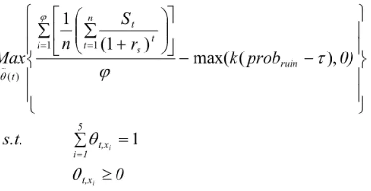
and ruin probability. The insurer prefers high expected discounted surplus but low ruin probability. More specifically, the optimization problem of the insurer is:
) _ ( )] ) 1 ( ) ( ( 1 [ 1 1 ) (
max
k ruin probability x I s t IS H I i H t t t − − +∑
∑
= = θK (8), where I is the number of the simulated paths in which no insolvency occurs, s is a constant chosen subjectively by the insurer to discount future surplus IS(t), k is also a constant chosen by the insurer to reflect the relative importance of excessive insolvency probability to expected discounted surplus, and x is the tolerable insolvency probability of the insurer.
The decision variable used to maximize the objective function is the asset allocation . Allocating more funds to high-risk types of assets may result in higher expected
surplus. It will however also result in higher ruin probability at the same time, which may not be optimal. A low ruin probability can be achieved by allocating more funds to low-risk assets. Such a strategy may not generate adequate returns for shareholders on the other hand. Therefore, the optimization problem can be deemed as a search for the optimal balance
between risk and return through asset allocation. )
(t
θK
In the following simulation, we set H at 25 years and the number of simulated paths at 5,000. The discount rate for future surplus per period s is assumed to be 3%, k is chosen to be
, and x = 2%. Without loss of generality of the multi-period asset allocation problem, we reduce the optimization problem from 25 years to 4 periods for the sake of computation time.
10
10
4×
15 More specifically, the insurer makes asset allocation decisions at t = 0, 6, 12, and 18,
and keeps the allocation the same as the previous year’s at all other times. The number of controllable variables is thus reduced to 12. A single-period asset allocation problem will have only three controllable variables, which may be solved using other simpler techniques.
III. THE SIMULATION OPTIMIZATION TECHNIQUES
A. An introduction to optimization via simulation
To solve the optimization problem set up in section II, we make use of the simulation optimization techniques. Optimization in the field of operations research has long been synonymous with mathematical programming. Due to the rapid advances in computational efficiency, there are now many techniques to optimize stochastic systems via simulation. Generally the problem setting is the following parametric optimization problem:
) ( max θ
θ∈ΘJ (9)
, where J(θ)=E[L(θ,ω)] is the performance measure of the problem, L(θ,ω) is called the sample performance, ω represents the stochastic effects of the system, θ is a p-vector of controllable variables, and Θ is the constraint set on θ. Let us also define the optimum as
. ) ( max arg * θ θ θ∈ΘJ =
Various simulation optimization techniques have been proposed to solve the above optimization problem. Several survey papers such as Fu (1994), Andradottir (1998), and Tekin and Sabuncuoglu (2004) have provided comprehensive coverage on the foundations, theoretical developments, and applications of these techniques. Existing techniques can be classified into two types: local optimization and global optimization. Local optimization techniques are further classified in terms of discrete and continuous decision spaces.16 Figure
1, copied from Tekin and Sabuncuoglu (2004), demonstrates the aforementioned classification scheme.
The major difference between local and global optimization techniques lies in the assumption about the shape of the response value surface, i.e., uni-modal or multi-modal. Local optimization techniques are therefore not suitable for those cases in which the function represented by the simulation model is complex and multimodal. These algorithms are
16 In a discrete space, decision variables take a discrete set of values such as the number of machines in a system.
The feasible region in a continuous space, on the other hand, consists of real-valued decision variables such as the release time of factory orders.
usually trapped in a local optimum and generate poor solutions, without an effective method to find good initial solutions. Global optimization techniques are developed to help a search escape from the local optimum. In the SCI and SSCI database we found over four thousand technical papers demonstrating that global optimization techniques such as tabu search, simulated annealing, and evolutionary algorithms can help the search escape from local optimum and produce better solutions.
Among the global optimization techniques, we chose evolutionary algorithms (EAs) for the DFA system. Using EAs in simulation optimization is on the increase lately because they require no restrictive assumptions or prior knowledge about the shape of the response surface (Back and Schwefel, 1993). In general, an EA has the following procedures: generate a population of solutions, evaluate these solutions through a simulation model, perform the selection, apply genetic operators to produce new offspring, and insert the new offspring into the population. These steps are repeated until some stopping criterion is reached.
The most popular EAs are genetic algorithms (GAs), evolution programming (EP), and evolution strategies (ES). These algorithms differ from each other in the representation of individuals, the design of variation operators, and the selection of their reproduction
mechanisms. In general, each point in the solution space is represented by a string of values for the decision variables. The crossover operator breaks the strings representing two members of the population and exchanges certain portions of the strings to create two new strings. The mutation operator selects a random position in a string and changes the value of that variable with a pre-specified probability. Appropriate crossover and mutation operators can reduce the probability of being trapped in a local optimum.
Among the GAs, EP, and ES, we chose to employ a GA to optimize the DFA system. The main reason for the choice was that GAs have found more applications for the optimizing problems in complex systems than either the EP or the ES. Also, we have applied GAs to several discrete optimization problems before (Chen et al. 1995, Chen et al. 1996, Chen et al.
2003). The following section gives a brief introduction on GAs and describes our GA in detail.
B. Genetic algorithms
The search procedure of GAs combines reproduction and recombination to mimic the process of natural evolution. An optimization problem solved by GAs can be explained as follows. The solution space of the problem is viewed as the environment of evolution. A solution of the problem is a member of a species in the environment. A generation of the species is presented as a population of solutions. Darwin's concept of survival of the fittest is then applied to the solutions in the population. The objective value of a solution is a measure of its fitness. The better the fitness of the solution, the higher the probability that the solution can be chosen as a parent to produce new solutions (offspring) for the next population
(generation). Genetic operators (usually crossover and mutation) have to be applied to the chosen parents to produce offspring. As this process continues for generations, the fitness of the members (objective values of solutions) improves.
Based on this explanation, the procedure of a basic genetic algorithm can be described as follows.17 Let S(t) denote the population in the t-th generation, si(t) the i-th member in S(t),
f(si(t)) the fitness of si(t), Totfit the sum of f(si(t)) in S(t), popsize the population size, and
maxgem the maximum number of generations for convergence. Then a GA usually has the
following steps.
Step 1: Generate an initial population, S(t), where t = 0.
Step 2: Calculate the fitness value for each member, f(si(t)), in population S(t).
Step 3: Calculate the selection probability for each member, which is defined as f(si(t))/Totfit.
Step 4: Select a pair of members (parents) randomly according to the selection probability. Step 5: Apply genetic operators to the parents to produce the offspring for the next population,
S(t+1). If the size of the new population is equal to popsize, then go to Step 6;
otherwise, go to Step 4.
Step 6: If the current generation, t+1, is equal to maxgen, then stop; else go to Step 2. According to the above basic procedure, the application of a GA must consider the following factors: (1) representation of a solution, (2) initial population, (3) selection probability, (4) genetic operators, (5) termination criterion, and (6) three parameters:
population size, crossover rate, and mutation rate. In the following, each of these factors and parameters will be discussed in detail for a GA to generate the optimal asset allocations
through our DFA system. 1. Representation of a solution
A solution for GA application is usually represented by a row vector. The value of an element in the vector refers to the allocation to an asset in a period. The number of elements in the vector depends upon the number of investable assets considered in a period and the number of periods considered in a problem. Since four assets are considered in four periods with the constraint that the sum of the allocations is equal to one, twelve elements are included in the vector in the current application.
2. Initial population
The initial population of our GA is randomly generated as most applications of GAs are. Since the value of an element in the vector is in the range of [0, 1], we first generate three
random numbers from the uniform [0, 1] distribution. If the sum of the three generated elements is greater than one, then the elements will be multiplied by 0.9 consecutively until their sum is less than or equal to one. We call this procedure a feasibility-keeping procedure. The purpose of the procedure is to ensure that the fourth element will not be negative and violate the short-sale constraint. Note that the feasibility-keeping procedure has to be implemented to all four periods in each vector.
3. Selection probability
performance measure of the member. Usually, a member with a better fitness in a population would have a higher probability of being selected. Since the candidate problem is to find an asset allocation that maximizes a specified utility function, the value of the utility function is used as the fitness value of the corresponding asset allocation. The larger the value of the utility function, the higher the probability the corresponding set of allocations will be selected. The following procedure is an application of the well-known roulette-wheel selection scheme for calculating the selection probability of a member in a population.
Step 1: Calculate the fitness f(i) for each member in the population.
Step 2: Calculate the total fitness, Totfit, of all the members in the population.
Step 3: Calculate the selection probability for each member that is equal to f(i)/Totfit.
A complementary selection strategy (elitist strategy) is also considered in the current application. More specifically, the member with the best fitness value in each population will always survive and automatically become a member in the next generation. The purpose is to preserve the best solution so that the search always covers certain good solution regions. 4. Genetic operators
Genetic operators are performed on the parents to generate offspring. Crossover and mutation are two common genetic operators of GAs.
4.1 Crossover
An effective crossover operator, BLX-0.5 (Eshelman & Schaffer, 1993), is used in this research. Two selected parents, vectors A and B, are given and denote the values of an element in A and B as x and y respectively. The BLX-0.5 is implemented to x and y in the following procedure to produce a value z for the element in the offspring generated by A and B. Step 1: Let ∆ = 0.5 ∗ |y-x|.
Step 2: Randomly generate z from the range of (x-∆, y+∆) if x ≤ y; let x-∆ = 0 if x-∆ < 0, and let
y-∆ = 0 if y-∆ < 0, and let x+∆ = 1 if x+∆ > 1.
For example, let (x1, x2) = (0.5, 0.2) be the values of the first two elements in A and let
(y1, y2) = (0.1, 0.8) be the values of the first two elements in B. The values of the first two
elements, (z1, z2) of the offspring of A and B can then be generated as follows. Let ∆1 = 0.5 ∗ | y1 – x1| = 0.5 ∗ |0.1 – 0.5| = 0.2 and ∆2 = 0.5 ∗ | y2 – x2| = 0.5 ∗ |0.8 – 0.2| = 0.3. Then
randomly generate z1 from the range of (y1-∆1, x1+∆1) = (0.1-0.2, 0.5+0.2) = (0, 0.7) and
randomly generate z2 from the range of (x2-∆2, y2+∆2) = (0.2-0.3, 0.8+0.3) = (0, 1.0).
4.2 Mutation
When a solution is produced by crossover, a mutation operator is applied to the solution. Michaleicz (1996) developed a non-uniform mutation operator and showed that the operator outperformed other mutation operators after performing thorough experiments. A
non-uniform mutation operator is applied in this GA application by following the procedure. Step 1: Randomly select k elements out of the 12 elements in the solution, where k = 1 +
Int[rnd*12] and Int is an integer function.
Step 2: Apply the non-uniform mutation operator to each of the k elements. It is given that element i is one of the k elements and is the value of element i in the current generation t. The value of element i in generation t+1, , is generated as follows:
= + ∆(t, 1.0 - ) if rnd < 0.5; otherwise = - ∆(t, ), where ∆(t, v) = v * (1.0 – rnd t i z 1 + t i z 1 + t i z t i z t i z t+1 i z t i z t i z
b), b = (1.0 – t/T)5, and T is equal to maxgen (the maximum number of
generations for convergence).
Note that b = (1.0 – t/T)5 is approaching 0 when t is close to T; when b is approaching 0, (t, v) also approaches 0. Michaleicz (1996) pointed out that this property causes the
non-uniform mutation operator to search uniformly the solution space initially (when t is small) and locally at later stages. Note also that after applying the mutation operator to the solution,
the feasibility-keeping procedure has to be implemented in the solution to maintain its feasibility.
4.3 Population size, crossover rate, and mutation rate
Population size (popsize) is the number of members generated in each generation. Crossover rate is the probability that a crossover operator applies to the chosen parents, and the mutation rate is the probability that a mutation operator applies to the offspring. The
population size of 60, as used in all the examples in Michaleicz (1996), is also used in the current application. Both crossover rate and mutation rate are set to be one after several trial runs for the candidate problem.
5. Termination Criteria
The maximum number of generations (maxgen) is the most widely used termination criterion for GAs. It is usually determined by trial-and-error. We found that our GA converged within 2000 iterations in all the trial runs in the current application. Therefore,
maxgen is set to be 2000.
We are now in a position to present the procedure of applying our GA to the DFA. Step 0: Let popsize = 60, maxgen = 2000, and t = 0.
Step 1: Generate initial population with twelve-element solutions (vectors) Vi (i = 1, 2, …,
popsize). For each solution, call rnd to generate an asset allocation to each of its
elements and apply the feasibility-keeping procedure to satisfy the constraint.
Step 2: Calculate the fitness, f(Vi), for each solution by conducting the DFA simulation with the
asset allocations given in Vi.
Step 3: Select two parent solutions based on their fitness. The selection probability of a parent solution Vi is p(i) = f(Vi)/Totfit.
Step 4: Apply crossover operator, BLX-0.5, to the selected parent solutions.
Step 5: Apply the non-uniform mutation operator to the solution generated in Step 4, and apply the feasibility-keeping procedure to maintain the feasibility of the solution.
Step 6: If the total number of offspring solutions generated is equal to popsize, go to Step 7; otherwise, go to Step 3.
Step 7: Let t = t + 1. If t is equal to maxgen, stop; otherwise go back to Step 2.
The optimization program is coded in C language and is executed using a Linux platform (the OS is the RedHat AS 3.0). The CPU is Intel Itanium 21.5GHz. One of the features of this optimization program is that the dynamics memory allocation is used for all the necessary variables. Therefore, the required memory used is around 70MB when running the program. The program is compiled using the Intel C/C++ compiler in the Linux System, yet it can also be compiled and executed using the Microsoft Window XP platform with Visual Studio C/C++ compiler. For 2000 iterations, this program took around 18,200 seconds to finish on average.
IV. RESULTS
A. General description of the DFA’s simulation results
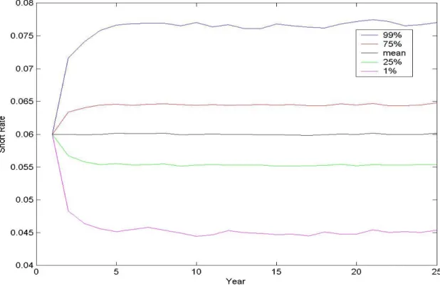
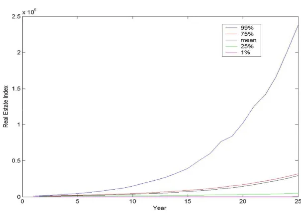
The simulated results of the financial markets are shown in Figures 2 to 4.18 We plot the simulated 1st percentile, 25th percentile, mean, 75th percentile, and 99th percentile values of each year in these figures. The mean of the simulated short rates remains at the long-term average value of 6%, with fifty percent of the simulated short rates falling within the range of 5.5% to 6.5%. The 1st percentile simulated short rates are about 4.5% while the 99th
percentile values are around 7.7%. The means of the equity index and real estate index display upward trends and the ranges of the simulated values widen as the simulation goes on, which is consistent with the specified stochastic processes.19
[Insert Figures 2 – 4 Here] B. Results of a basic search method
18 The simulation results of the insurance markets are not reported because the simulation is straightforward. The
loss ratio of each year is drawn from a normal distribution.
19 We have also inspected the figures of the equity returns and real estate returns (not shown in the paper). The
25th percentile, mean, 75th percentile values of equity returns remain at -0.1%, 12%, 24% respectively across time.
The minima and maxima of equity returns exhibit some bumps around -60% and 80%, respectively. Real estate returns display similar features with higher means and wider variation ranges.
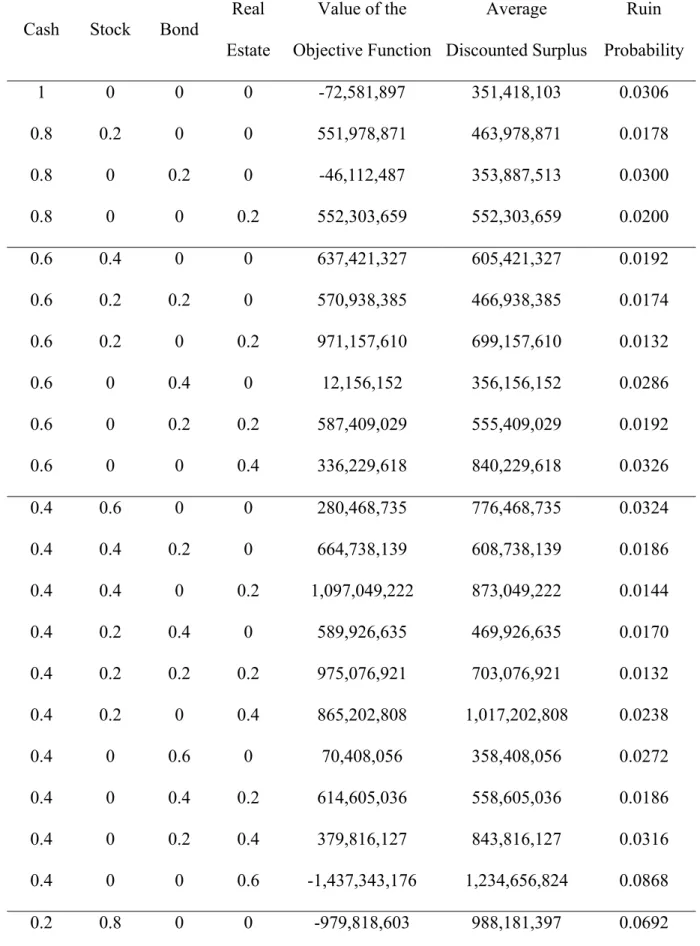
Before using the simulation optimization technique, we tried out a basic search method in a single-period framework as follows. We list all possible asset allocations using the grid size of 20%. Inserting these allocations into the DFA system and assuming that these
allocations are kept to the end of the simulation, we obtain the values of the objective function. These values along with their associated average discounted surpluses as well as ruin
probabilities are shown in Table 1.
[Insert Table 1 Here]
Table 1 shows that the best asset allocation is θK*(t)=
[
0 0.4 0.4 0.2]
′. It results in an objective function value of 1,137,275,044 with an average discounted surplus of$881,275,044 and a ruin probability of 1.36%. Although the zero-cash allocation looks odd, it is reasonable because we did not consider liquidity in the model setting. Furthermore, new premiums can cover the loss payments in most cases. The runner-up is
[
′= 0.2 0.4 0.2 0.2 )
(t
θK
]
with an objective function value of 1,132,889,250, an average discounted surplus of $876,889,250, and a ruin probability of 1.36%. The runner-upallocation generates a little bit less expected surplus, which is reasonable because the return on cash on average is smaller.20 Number three is θK(t)=
[
0.4 0.4 0 0.2]
′ which results in an objective function value of 1,097,049,222, an average discounted surplus of $873,049,222, and a ruin probability of 1.44%. The higher insolvency probability is probably because cash does not generate adequate returns. Number four is θK(t)=[
0 0.2 0.6 0.2]
′. This asset allocation produces an objective function value of 1,022,434,859, an average discounted surplus of $710,434,859, and a ruin probability of 1.22%. Although it generates the smallest ruin probability among all the asset allocations, it produces an inferior average discounted
20 Remember that the return from cash is the one-year short rate. Since the simulated yield curve is usually
upward-sloping, the one-year bond is smaller than longer-maturity bonds. The insolvency probability of the runner-up is the same as the number-one choice implies that the risk of the bond portfolio is small.
surplus compared to the top three allocations. The fifth winner is θK(t)=
[
0 0.4 0.2 0.4]
′ which results in an objective function value of 1,017,769,551, an average discounted surplus of $1,225,769,551, and a ruin probability of 2.52%. Allocating more assets to higher-riskequities produces a significantly higher average surplus, but results in a higher ruin probability. The ranking of the top five asset allocation looks reasonable. However, we do not spot any pattern revealing between which two asset allocations the optimal allocation might be. Weighting three variables to balance a higher average surplus with lower ruin probability is rather difficult. Reducing the grid size of 20% is therefore the way to go if we do not have any algorithm to search for the optimum. However, this reduction will increase the possible asset allocation dramatically. When the grid size is 20%, the total number of asset allocations is 56. When the grid size is 10%, the number increases to 286. Five percent of grid size will produce 1,771 combinations while one percent will result in 176,851 allocations. Therefore, the basic search method is not feasible in finding the optimal asset allocation even though it is intuitive and instructive.
C. Results of the genetic algorithm
Our GA produces a significantly better result than the basic search method. The value of the objective function is 1,343,396,299 implying an 18% improvement over the above basic search method. The GA results in a significantly higher average discounted surplus
($1,055,396,299 that is 20% higher than that of the winner in section B) and a lower ruin probability (1.28%). The optimal asset allocation is as follows:
t 0 6 12 18
Cash 16.1906% 2.7821% 14.4054% 3.3340%
Stock 32.4451% 45.2235% 47.1426% 40.3112%
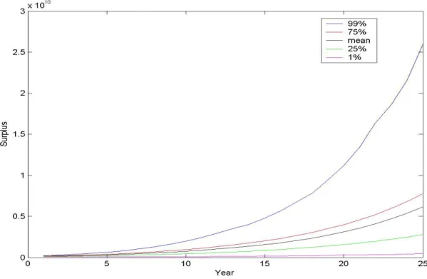
Real Estate 21.7216% 39.2053% 32.7491% 49.2814% . We plotted the resulting 1st percentile, 25th percentile, mean, 75th percentile, and 99th percentile surplus over time from the optimal asset allocation in Figure 5.
[Insert Figure 5 Here]
To secure the robustness of our application of GA to DFA, we tried two other sets of random numbers and two other sets of parameters of the underlying risk models.21 Using different sets of random number results in small changes in the objective function value.22 The resulting values are 1,338,413,716 and 1,358,066,783. Since these values represent a -0.37% and 1.09% difference respectively from the benchmark case described in the previous one paragraph, our application is robust across random numbers.
The other two sets of parameters generate significantly different results. Alternative parameter set 1 resulted in an objective function value of 1,445,571,649, an average discounted surplus of $829,571,650, and a ruin probability of 0.46%. The optimal asset allocation is as follows: t 0 6 12 18 Cash 34.4349% 18.2585% 0.1492% 2.5802% Stock 19.6516% 15.9641% 36.8198% 49.8485% Bond 17.8915% 30.4849% 2.1546% 10.3742% Real Estate 28.0221% 35.2925% 60.8764% 37.1971% . The features of this parameter set include fairly profitable but highly volatile financial as well as insurance markets with a moderately positive correlation between the long-tail insurance and financial markets. The position correlation possibly contributes to the lower
21 The alternative parameter sets are described in the appendix.
22 The two alternative parameter sets are specified rather arbitrarily. We intentionally make them “unreasonable”
to see whether our GA can still find solutions under odd settings. The random number set used for these two alternative parameter sets is the same as the one used in the benchmark case.
ruin probability compared to that in the benchmark case and thus generates a higher objective function value. The lower average discounted surplus might be as a result from the relatively conservative investments during the first twelve years.
Alternative parameter set 2 results in an objective function value of 998,583,316, an average discounted surplus of $198,583,316, and zero ruin probability. The optimal asset allocation is as follows: t 0 6 12 18 Cash 0.0010% 0.0010% 0.0010% 0.0183% Stock 14.3156% 17.6433% 25.7770% 21.0308% Bond 0.0010% 0.0013% 0.0053% 0.1233% Real Estate 85.6824% 82.3544% 74.2167% 78.8276% . The features of alternative parameter set 2 include highly positive correlations between the long-tail insurance and the financial markets, relatively safe insurance markets, a fairly
profitable but highly volatile stock market, and a low-return but high-risk bond market. The allocations to bonds and cash are thus minimal. Most of the funds are allocated to real estate with some funds to stocks for higher returns. The average discounted surplus under
parameter set 2 is the smallest among the three parameter sets because the discount rate for surplus is the highest (45% vs. 3% and 15%). The lower returns in the financial markets might also contribute to the smallest average discounted surplus. The zero insolvency probability is probably due to the low risk in the insurance markets and the high correlation between the financial and long-tail insurance markets. Finally, the significantly lower average discounted surplus under parameter set 2 compared to the other two parameter sets results in the smallest objective among the three parameter sets.
Managing an insurance company is more difficult than managing other types of companies because an insurer faces not only asset risks but also liability risks. The DFA system is a promising tool for the insurer. It takes full account of the static and dynamic relations among asset variables and liability variables. The major output of a DFA system is the distribution of an insurer’s future surplus that can be further used to compare alternative asset allocations, business strategies, and reinsurance arrangements, among others. Insurance regulators can use a DFA system to perform an early warning analysis as well as set up
minimal capital requirements.
The main drawback of the DFA system is the lack of an optimization mechanism. Users can perform only comparative analysis with no way of knowing what the optimal strategy is. Simulation optimization is receiving considerable interest in the field of operations research and may be a nice complement to the DFA system. By incorporating optimization features in a DFA system, the DFA system turns from a descriptive model into an operational tool to solve various decision-making problems. The contribution of this paper is coupling a DFA system with a simulation optimization technique and applying the combination to the asset allocation problem of a property-casualty insurance company.
We first built up a simply DFA system in which an insurer underwrites both short- and long-tail businesses and invest in four types of assets. Then we formulated the asset
allocation problem as a multi-period one instead of a single-period one. A multi-period asset allocation is superior because the accumulation of a sequence of single-period optimal
decisions across periods may not be optimal for these periods taken as a whole. We also considered the short-sale constraints faced by insurers when making investments. The
capability of solving a constrained multi-period problem illustrates the advantage of simulation optimization, although we must keep in mind that the found solution as a result of simulation optimization cannot be proved to be the optimum. The simulation optimization technique used in this paper is a generic algorithm.
We successfully incorporated a generic algorithm into a DFA system and performed a search for the optimal asset allocation of a property-casualty insurer in this paper. The
resulting asset allocation was a significantly higher value of the objective function compared to the allocation found from a basic search method. The optimal allocation produced a higher average discounted surplus and a lower ruin probability. Using different sets of random number generated similar values of objective function and demonstrated the robustness of our coupling across random numbers. The optimal asset allocation is sensitive to the parameters of financial and insurance market models, with the changes being consistent with the
differences in the parameters. Therefore, insurance companies that are using or are interested in DFA should learn one of the simulation optimization techniques to equip their DFA systems with optimization features.
References
Andradottir, S., 1998. Simulation Optimization. In: Handbook of Simulation: Principles, Methodology, Advances, Applications, and Practice. Wiley, New York, pp. 307-333. Back, T., Schwefel, H. P., 1993. An overview of evolutionary algorithms for parameter
optimization. Evolutionary Computation 1, 1-23.
Chen, C. L., Vempati, V. S., Aljaber, N., 1995. An application of genetic algorithms for flow shop problems. European Journal of Operational Research 80, 389-396.
Chen, C. L., Neppalli, V. R., Aljaber, N., 1996. Genetic algorithms applied to the continuous flow shop problem. Computers and Industrial Engineering 30, 919-929.
Chen, C. L., Lin, R. H., Zhang, J., 2003. Genetic algorithms for MD-optimal follow-up designs. Computers & Operations Research 30, 233-252.
Coutts, S. M., Devitt, R., 1989. The Assessment of the Financial Strength of Insurance Companies by a Generalized Cash Flow Model. In: Financial Models of Insurance Solvency. Kluwer Academic Publishers, Boston, pp. 1-36.
Econometrica 53, 385-407.
Cummins, J. D., Grace, M. F., Phillips, R. D., 1999. Regulatory solvency prediction in property-liability insurance: risk-based capital, audit ratios, and cash-flow simulation. Journal of Risk and Insurance 66, 417-458.
Daykin, C. D., Bernstein, G. D., Coutts, S. M., Devitt, E. R. F., Hey, G. B., Reynolds, D. I. W., Smith, P. D., 1989. The Solvency of a General Insurance Company in Terms of Emerging Costs. In: Financial Models of Insurance Solvency. Kluwer Academic Publishers, Boston, pp. 87-149.
Daykin, C. D., Hey, G. B., 1991. A Management Model of a General Insurance Company Using Simulation Techniques. In: Managing the Insolvency Risk of Insurance Companies. Kluwer Academic Publishers, Boston, pp. 77-108.
Daykin, C. D., Pentikainen, T., Pesonen, M., 1994. Practical Risk Theory for Actuaries. Chapman & Hall, London.
Eshelman, L. J., Schaffer, J. D., 1993. Real-Coded Genetic Algorithms and Interval Schemata. In: Foundations of Genetic Algorithms. Morgan Kaufmann Publishers, San Mateo, pp. 187-202.
Fu, M. C., 1994. Optimization via simulation: a review. Annals of Operations Research 53, 199-247.
Keys, A. C., Rees, L. P., 2004. A sequential-design metamodeling strategy for simulation optimization. Computers and Operations Research 31, 1911-1932.
Michalewicz, Z., 1996. Genetic Algorithms + Data Structures = Evolution Programs, 3rd ed. Springer-Verlag, Berlin.
Paulson, A. S., Dixit, R., 1989. Cash Flow Simulation Models for Premium and Surplus Analysis. In: Financial Models of Insurance Solvency. Kluwer Academic Publishers, Boston, pp. 37-56.
Theory. Kluwer Academic Publishers, Boston, pp. 1-48.
Taylor, G., 1991. An Analysis of Underwriting Cycles and their Effects on Insurance Solvency. In: Managing the Insolvency Risk of Insurance Companies. Kluwer Academic Publishers, Boston, pp. 3-76.
Taylor, G. C., Buchanan, R., 1988. The Management of Solvency. In: Classical Insurance Solvency Theory. Kluwer Academic Publishers, Boston, pp. 49-155.
Tekin, E., Sabuncuoglu, I., 2004. Simulation optimization: a comprehensive review on theory and applications. IIE Transactions 36, 1067-1081.
Table 1: The results of the basic research method
Cash Stock Bond Real Estate Value of the Objective Function Average Discounted Surplus Ruin Probability 1 0 0 0 -72,581,897 351,418,103 0.0306 0.8 0.2 0 0 551,978,871 463,978,871 0.0178 0.8 0 0.2 0 -46,112,487 353,887,513 0.0300 0.8 0 0 0.2 552,303,659 552,303,659 0.0200 0.6 0.4 0 0 637,421,327 605,421,327 0.0192 0.6 0.2 0.2 0 570,938,385 466,938,385 0.0174 0.6 0.2 0 0.2 971,157,610 699,157,610 0.0132 0.6 0 0.4 0 12,156,152 356,156,152 0.0286 0.6 0 0.2 0.2 587,409,029 555,409,029 0.0192 0.6 0 0 0.4 336,229,618 840,229,618 0.0326 0.4 0.6 0 0 280,468,735 776,468,735 0.0324 0.4 0.4 0.2 0 664,738,139 608,738,139 0.0186 0.4 0.4 0 0.2 1,097,049,222 873,049,222 0.0144 0.4 0.2 0.4 0 589,926,635 469,926,635 0.0170 0.4 0.2 0.2 0.2 975,076,921 703,076,921 0.0132 0.4 0.2 0 0.4 865,202,808 1,017,202,808 0.0238 0.4 0 0.6 0 70,408,056 358,408,056 0.0272 0.4 0 0.4 0.2 614,605,036 558,605,036 0.0186 0.4 0 0.2 0.4 379,816,127 843,816,127 0.0316 0.4 0 0 0.6 -1,437,343,176 1,234,656,824 0.0868 0.2 0.8 0 0 -979,818,603 988,181,397 0.0692
0.2 0.6 0.2 0 331,768,042 779,768,042 0.0312 0.2 0.6 0 0.2 920,627,902 1,072,627,902 0.0238 0.2 0.4 0.4 0 707,867,321 611,867,321 0.0176 0.2 0.4 0.2 0.2 1,132,889,250 876,889,250 0.0136 0.2 0.4 0 0.4 996,985,281 1,220,985,281 0.0256 0.2 0.2 0.6 0 585,128,292 473,128,292 0.0172 0.2 0.2 0.4 0.2 1,002,693,284 706,693,284 0.0126 0.2 0.2 0.2 0.4 916,984,155 1,020,984,155 0.0226 0.2 0.2 0 0.6 -262,968,275 1,425,031,725 0.0622 0.2 0 0.8 0 120,775,989 360,775,989 0.0260 0.2 0 0.6 0.2 641,808,556 561,808,556 0.0180 0.2 0 0.4 0.4 423,394,768 847,394,768 0.0306 0.2 0 0.2 0.6 -1,377,259,696 1,238,740,304 0.0854 0.2 0 0 0.8 -4,699,438,942 1,764,561,058 0.1816 0 1 0 0 -3,230,097,737 1,249,902,263 0.1320 0 0.8 0.2 0 -881,219,802 990,780,198 0.0668 0 0.8 0 0.2 192,104,867 1,304,104,867 0.0478 0 0.6 0.4 0 351,750,776 783,750,776 0.0308 0 0.6 0.2 0.2 948,987,876 1,076,987,876 0.0232 0 0.6 0 0.4 608,774,850 1,456,774,850 0.0412 0 0.4 0.6 0 727,242,728 615,242,728 0.0172 0 0.4 0.4 0.2 1,137,275,044 881,275,044 0.0136 0 0.4 0.2 0.4 1,017,769,551 1,225,769,551 0.0252 0 0.4 0 0.6 -153,875,069 1,662,124,931 0.0654 0 0.2 0.8 0 604,121,085 476,121,085 0.0168
0 0.2 0.6 0.2 1,022,434,859 710,434,859 0.0122 0 0.2 0.4 0.4 953,078,642 1,025,078,642 0.0218 0 0.2 0.2 0.6 -187,400,811 1,428,599,189 0.0604 0 0.2 0 0.8 -3,183,750,687 1,968,249,313 0.1488 0 0 1 0 131,373,027 363,373,027 0.0258 0 0 0.8 0.2 661,117,051 565,117,051 0.0176 0 0 0.6 0.4 451,314,002 851,314,002 0.0300 0 0 0.4 0.6 -1,309,777,975 1,242,222,025 0.0838 0 0 0.2 0.8 -4,639,208,243 1,768,791,757 0.1802 0 0 0 1 -8,421,281,758 2,482,718,242 0.2926
Optimization Problems
Local Optimization
Discrete Decision Space
Continuous Decision Space
Figure 1: Classification of optimization methodologies
Figure 2: The simulated short rate statistics along with time
Global Optimization
Ranking and Selection
Response Surface Methodology Multiple Comparison
Ordinal Optimization
Finite Difference Estimates Random Search
Perturbation Analysis Simplex/Complex Search
Likelihood Ratio Estimates Stochastic Approximation Single Factor Method
Hooke-Jeeves Pattern Search
Evolutionary Algorithms Tabu Search
Simulated Annealing
Bayesian/Sampling Algorithms Gradient Surface Method